Mathematical Perspectives in the Variable Texture Products Cutting Process

Abstract

The methods utilized to construct and identify the mathematical equation that characterizes the cutting of items with varied textures are presented in this work. Using laboratory equipment, the cutting process was carried out experimentally. The cutting energy was calculated based on the experimental results. The energy required to perform this process is directly influenced by the textural characteristics of the products used, as per the analysis of the experimental results obtained after the cutting process (density, humidity, products with or without peel). The gathered information was used to develop a general equation that would properly describe the process. Table Curve 3D software was used to create mathematical equations that define the relationship between input parameters, the type of product being cut, cutting speed, and output parameters, i.e., cutting energy. The equations that have the same correlation coefficient were discovered using the working methodology; it was specifically designed for this purpose.

1. Introduction

Because agri-food products are varied and have characteristics that change over time and location, cutting them is a highly difficult task.

Cutting solid materials is common and important due to the large quantities of raw materials and processed products, as well as the energy consumption, of which only a small fraction (0.1–0.2%) is used to overcome the cohesive forces in the particles, with the rest dissipating unnecessarily and even harmfully in the form of heat [1,2,3].

Prior to determining the conditions under which the cutting process will be carried out with maximum efficiency, it is necessary to have a solid understanding of the characteristic indices of the products to be cut (raw material properties, required quality conditions, properties related to the texture of the products to be shredded), as well as their effect on the cutting process. Many specialized studies have shown that as moisture content increased, so did specific energy consumption [4,5,6].

Particle cutting requires a certain amount of energy. The specific energy consumption (J/kg) in the cutting process reflects the amount of energy required to achieve a specified degree of cutting off the unit mass of the product under cut [2,3,7]. The nature of the material being ground, its initial state, structure, and internal condition, the size, speed, and duration of the mechanical stress applied, the nature of the forces applied, the particle size before and after cutting, and the cutting degree are all factors that affect this process [8,9,10,11,12,13].

The energy consumed during the cutting process is only partially usable; the remainder goes to the development of elastic and plastic deformations in the cutting material, particle friction between themselves and the machine’s active organs, and internal mechanical losses [8,14,15,16,17,18].

Cutting is an inefficient process in terms of energy consumption. There is no clear method of calculating the minimum amount of energy necessary for cutting, however, numerous hypotheses have been proposed [16,17,18,19,20].

Many of the equations for calculating cutting energy that has been developed in the literature are empirical [1,3,9,10]. The three cutting equations that exist in the literature are based on a hypothesis that has received a lot of attention in the literature [8,15,17,18,20,21,22,23,24].

Bond correlates the energy for shredding to the size of a single particle. According to Kick, the energy of the particles is proportionate to their volume [17,18]. Rittinger believes that the amount of energy spent during the cutting process is proportionate to the new surface formed throughout the cutting process [1,3,17,18,21,23,24]. Each of the three equations has a specific constant, the value of which must be calculated from experimental data. The following is how Rittinger’s connection for agri-food items with a variable texture was employed in this study:

$$E_R=k_R\left(\frac{1}{d}-\frac{1}{D}\right)$$

(1)

in which: D is the average size of the material to be cut; d is the average size of the cutting material; k_R is Rittinger’s constant, considered as:

$$k_R=F_m\cdot S_n$$

(2)

where: F_m is the cutting force, S_n is the new surface created.

The next stage in working with experimental data, according to the literature, is to identify the mathematical equations that describe the correlations between the input and tracked parameters [25,26,27,28,29,30,31,32,33,34].

In the specialized literature, there are a lot of experiments that deal with the cutting process and the identification of the mathematical equations that describe this process. However, these equations are generated for specific cases. In conclusion, the purpose of this paper was to develop a general equation that described the relationships between the operating parameters of the cutting equipment and the energy required to fulfill the process (value defined by relation (1)). The mathematical equations that have been chosen to describe the cutting process have resulted from a methodology that can give the equations obtained a general character. An approach for processing the set of equations generated by Table Curve 3d software was created and designed for this purpose [35].

2. Materials and Methods

The investigation was conducted using a texture analyzer to determine the energy required to accomplish the cutting operation for various products. Texture Profile Analysis (TPA) is an objective method of sensory analysis developed by Szczesniak in 1963. He was the first to specify the textural parameters for this method. This method (Texture Profile Analysis-TPA) is based on the concept that texture is a highly influenced characteristic by a variety of factors [3,17,18,21,23,24].

The “Texture Analyzer-TA-XT2i” measurement equipment is used for this (Figure 1a,b) because it gives a three-dimensional study of the cutting force based on the knife’s stroke during the cutting process and the cutting time.

Cohesion, reliability, elasticity, freshness, breaking strength, penetration strength, expansion strength, adhesiveness, ability to masticate, and other tests may be assessed using the device and the “Texture Expert” application [14,16,17,18]. As a cutting device, the sample type HDP/BS was used in this investigation (Figure 1b,c).

Different species and varieties of vegetables and fruits were chosen to represent a wide variety of vegetable items with a texture liked by the descriptor “hard” in order to carry out the study regarding the process of cutting experiments. The species and varieties for which the determinations were performed are shown in

Table 1. Texture analysis was conducted to analyze various fruit species and varieties [22].

Item No.	Species	Variety	Maturity	Observation
1.	Apple	Grave Steiner	Complete	Unpeeled
2.	Apple	Grave Steiner	Complete	Peeled
3.	Apple	Ida Red	Complete	Unpeeled
4.	Apple	Ida Red	Complete	Peeled
5.	Apple	Golden Delicious	Complete	Unpeeled
6.	Apple	Golden Delicious	Complete	Peeled
7.	Apple	Jonagold	Complete	Unpeeled
8.	Apple	Jonagold	Complete	Peeled
9.	Pear	Clapp’s Favorite	Ripen	Unpeeled
10.	Pear	Clapp’s Favorite	Ripen	Peeled

and

Table 2. Vegetable species and varieties analyzed by the method of texture analysis [22].

Item No.	Species	Variety	Maturity	Observation
1.	Potato	Désirée	Complete	Unpeeled
2.	Potato	Désirée	Complete	Unpeeled
3.	Potato	Sante	Complete	Unpeeled
4.	Potato	Sante	Complete	Peeled
5.	Carrot	Nassan	Complete	Unpeeled
6.	Carrot	Nassan	Complete	Peeled
7.	Celery	Victoria	Complete	Unpeeled
8.	Celery	Victoria	Complete	Peeled
9.	Parsnip	Long White	Complete	Unpeeled
10.	Parsnip	Long White	Complete	Peeled

.

The parameters of the investigated products vary depending on the species and variety.

Table 3. The average density and average humidity of the fruits that have been analyzed [22].

Item No.	Species	Density (kg/m3)	Humidity (%)
1.	Apple	790	88.5
2.		846	87.5
3.		920	84.1
4.		930	83.5
5.	Pear	1028	85.1

and

Table 4. The average density and average humidity of the vegetables were investigated [22].

Item No.	Species	Density (kg/m3)	Humidity (%)
1.	Potato	1010	82.3
2.		1050	74.5
3.		1060	79.6
4.	Carrot	1040	88.8
5.	Celery	964	87.0
6.	Parsnip	994	89.5

show the average humidity and density for the investigated varieties.

The following conclusions can be derived from the examination of the parameters that characterize the products that will be subjected to the analysis:

-

The variation of their density is inversely proportional to the variation of the humidity in the case of the apple product used in these experimental determinations;

-

In the case of the potato product, it was found that the lowest product density is associated with the highest humidity. The lowest value of the parameter studied was obtained for the next value of the density of the studied product, and for the highest value of the density, it was found that the humidity is higher by 5.1% compared to the minimum value;

-

Because we only have one sample of the other products used in the study, no relevant conclusions can be drawn.

The investigations were carried out in accordance with the working technique represented in Figure 2.

3. Results

Following the replacement of the experimental results obtained under Equation (1), a series of cutting energy values were produced, which are represented graphically in Figure 3, Figure 4, Figure 5, Figure 6, Figure 7, Figure 8, Figure 9 and Figure 10.

The study of the results obtained by using the texture analysis approach to determine the cutting energy reveals that:

-

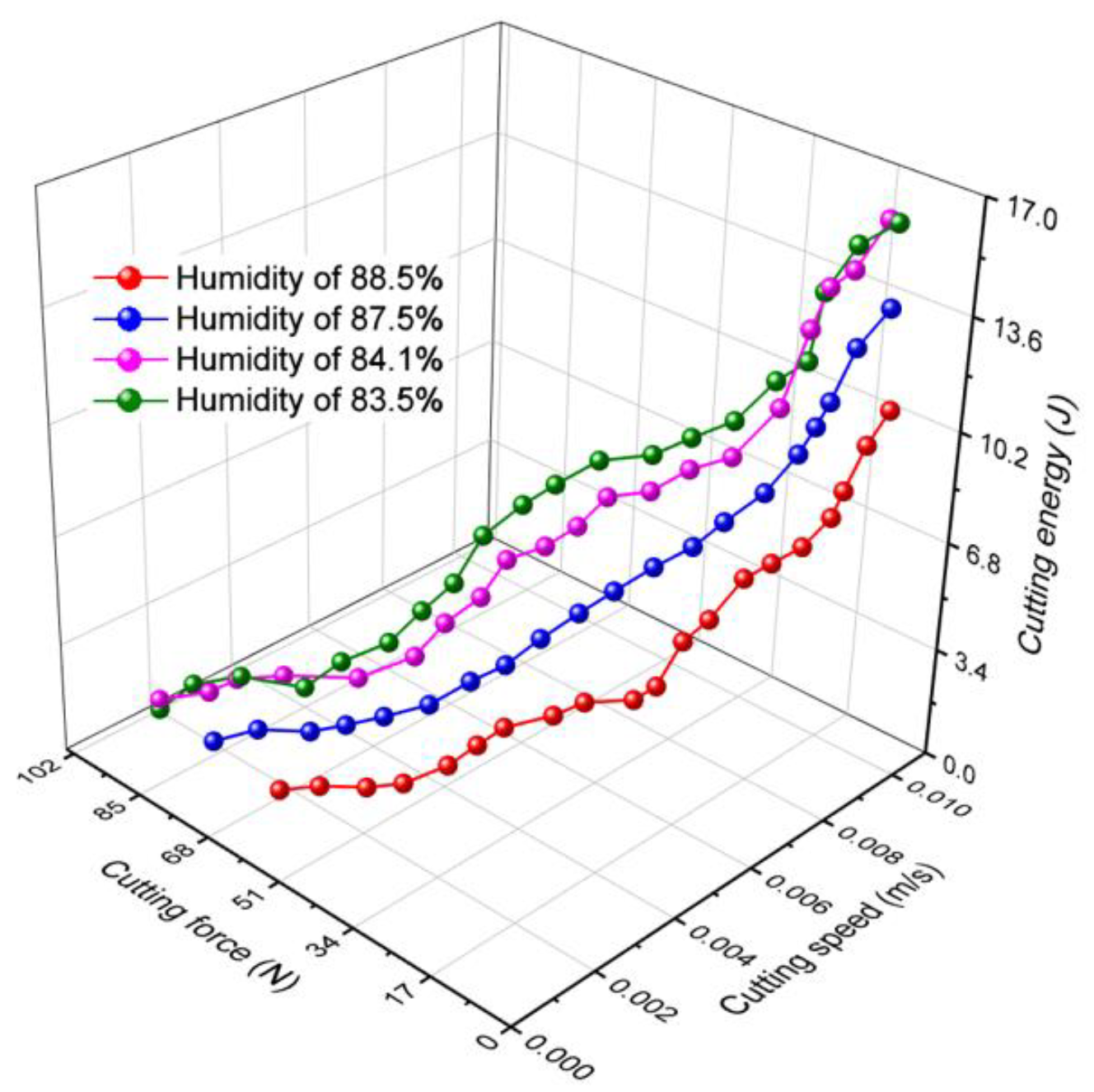
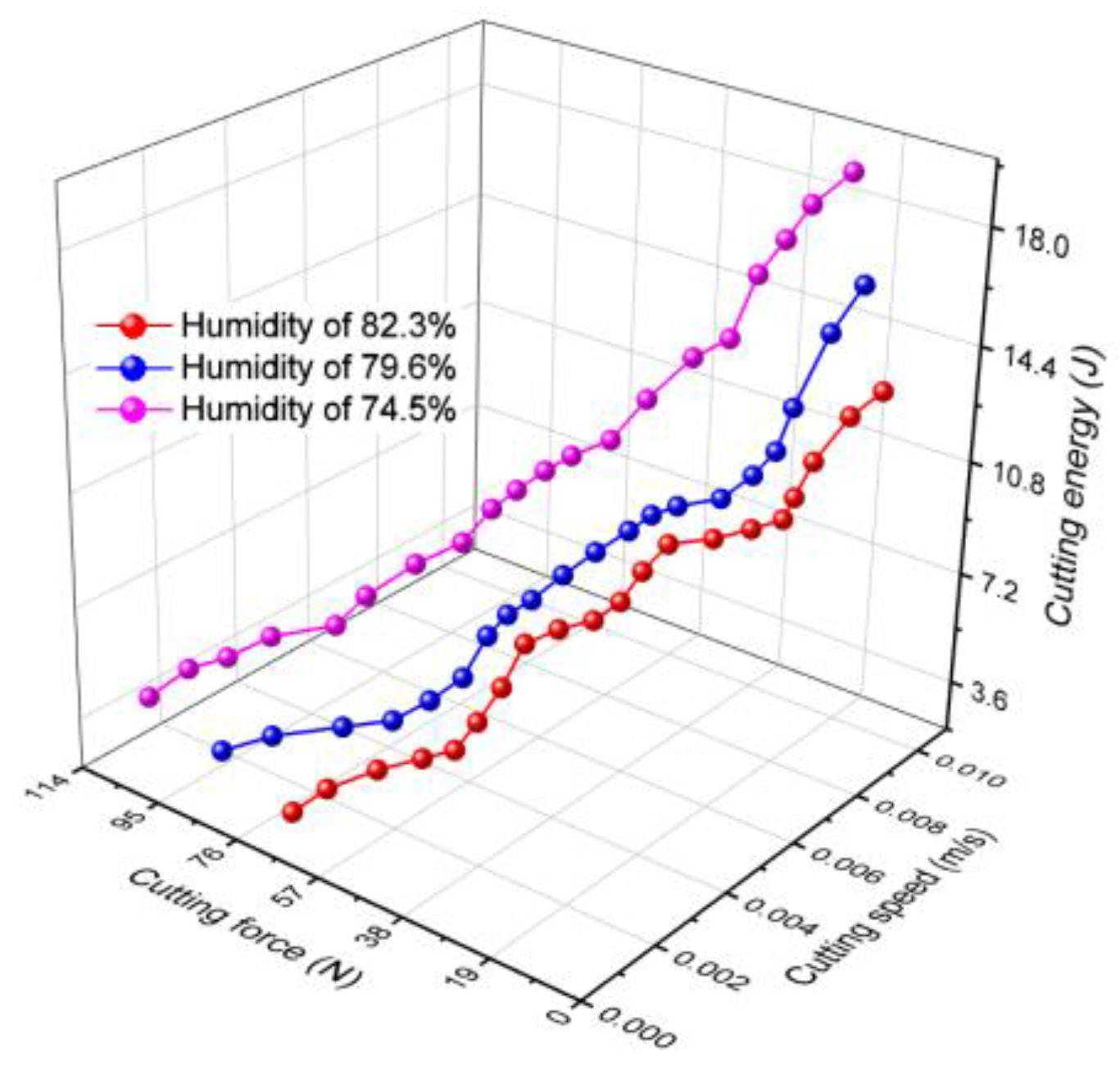
the textural properties of the products to be cut (humidity of the products) influence the cutting process; high cutting energy values have been obtained for products with low humidity;

-

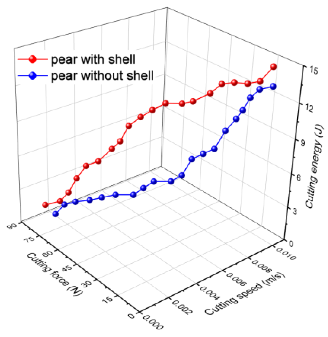
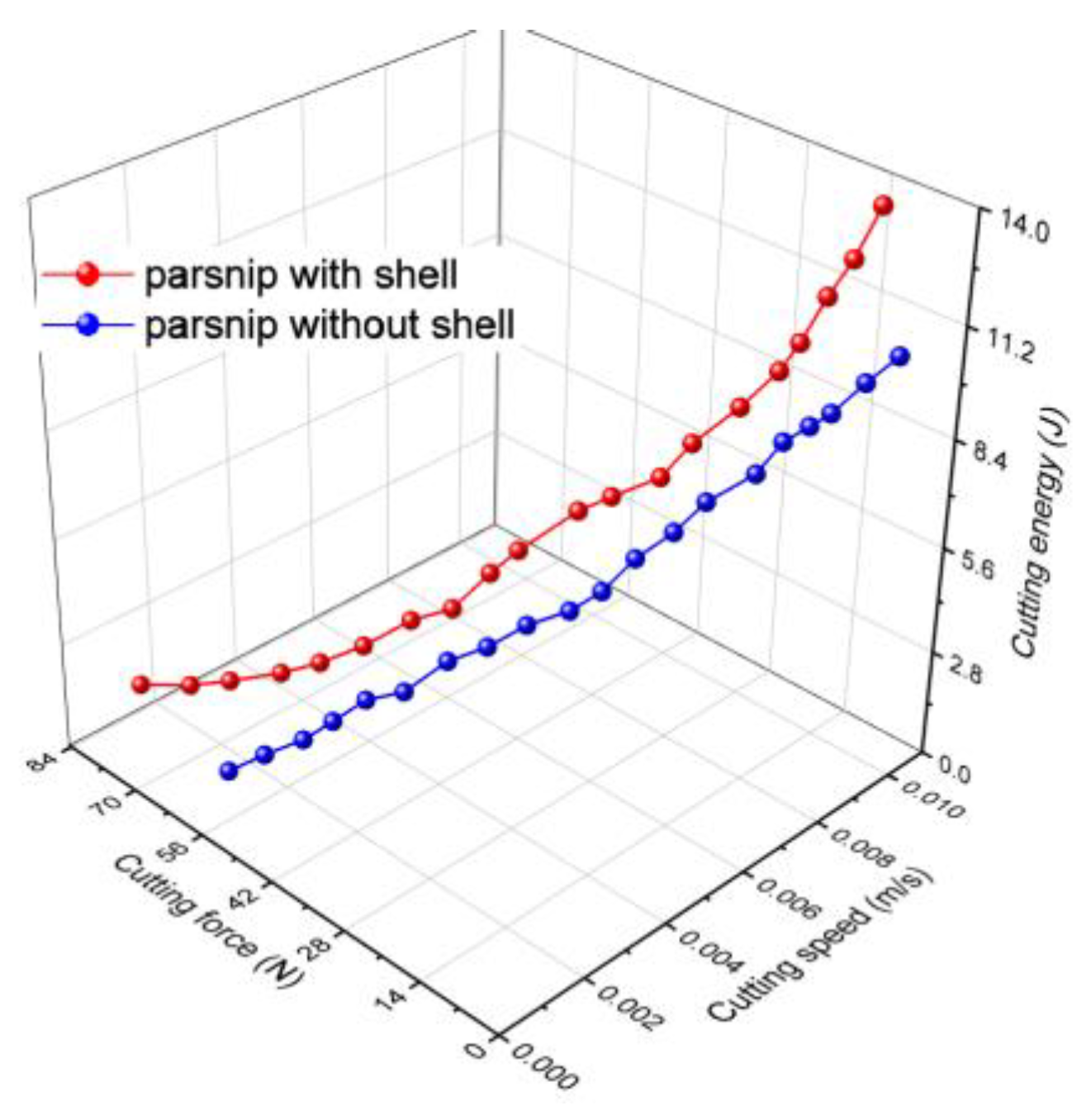
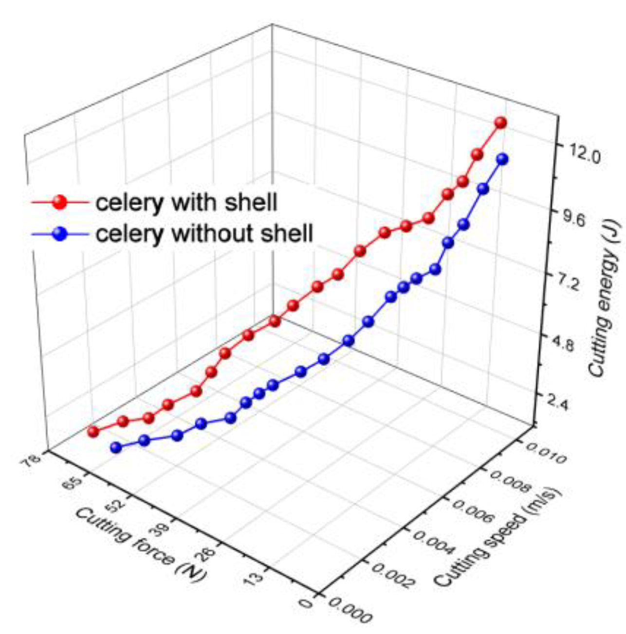
The condition of the products to be cut has an impact on the cutting energy. According to the results of the experiments, when cutting unpeeled products, higher values of cutting energy were achieved than when cutting peeled products;

-

The condition of the products being cut affects the cutting energy. When examining the obtained data, it is evident that there are small variations in cutting energy for small values of cutting speed, which can be seen when comparing unpeeled and peeled products, suggesting that the cutting energy for the same products tends to increase in direct proportion to the cutting speed. This is also confirmed by numerous field research, such as in the case of wheat straw cutting [7];

-

Within the same species, cutting energy varies depending on variety, with the difference being mostly attributable to the textural characteristics, as shown in the case of celery, which has the biggest range of cutting energy observed, with its structure changing from the outside to the inside.

4. Generating Mathematical Equations

The values obtained and represented in Figure 3, Figure 4, Figure 5, Figure 6, Figure 7, Figure 8, Figure 9 and Figure 10 were used to determine the correlations between the current study’s input parameters (cutting speed and cutting force) and the output parameters (cutting energy).

Given its ability to generate over 30,000 types of equations, Table Curve 3D software was utilized to obtain these relationships [37].

The following are the actions that were taken in order to determine the mathematical equations that corresponded to the study that was conducted (Figure 11):

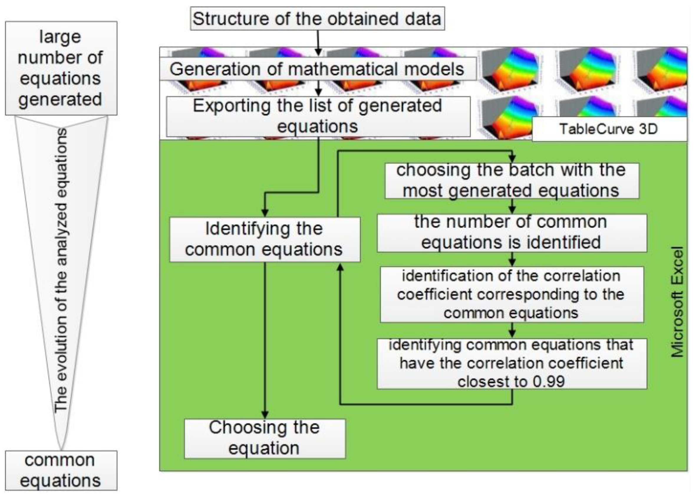
• The experimental values obtained are inserted into an excel file, and the data are arranged in separate columns;
• Table Curve 3D program allows the insertion of this excel file carrying data;
• The parameters corresponding to the three axes are selected where, on the OX (cutting speed) and OY (cutting force) axes, the input parameters are introduced, while on the OZ (cutting energy) axis the tracked parameter is introduced;
• Table Curve 3D software can generate equations that correlate to the values entered.
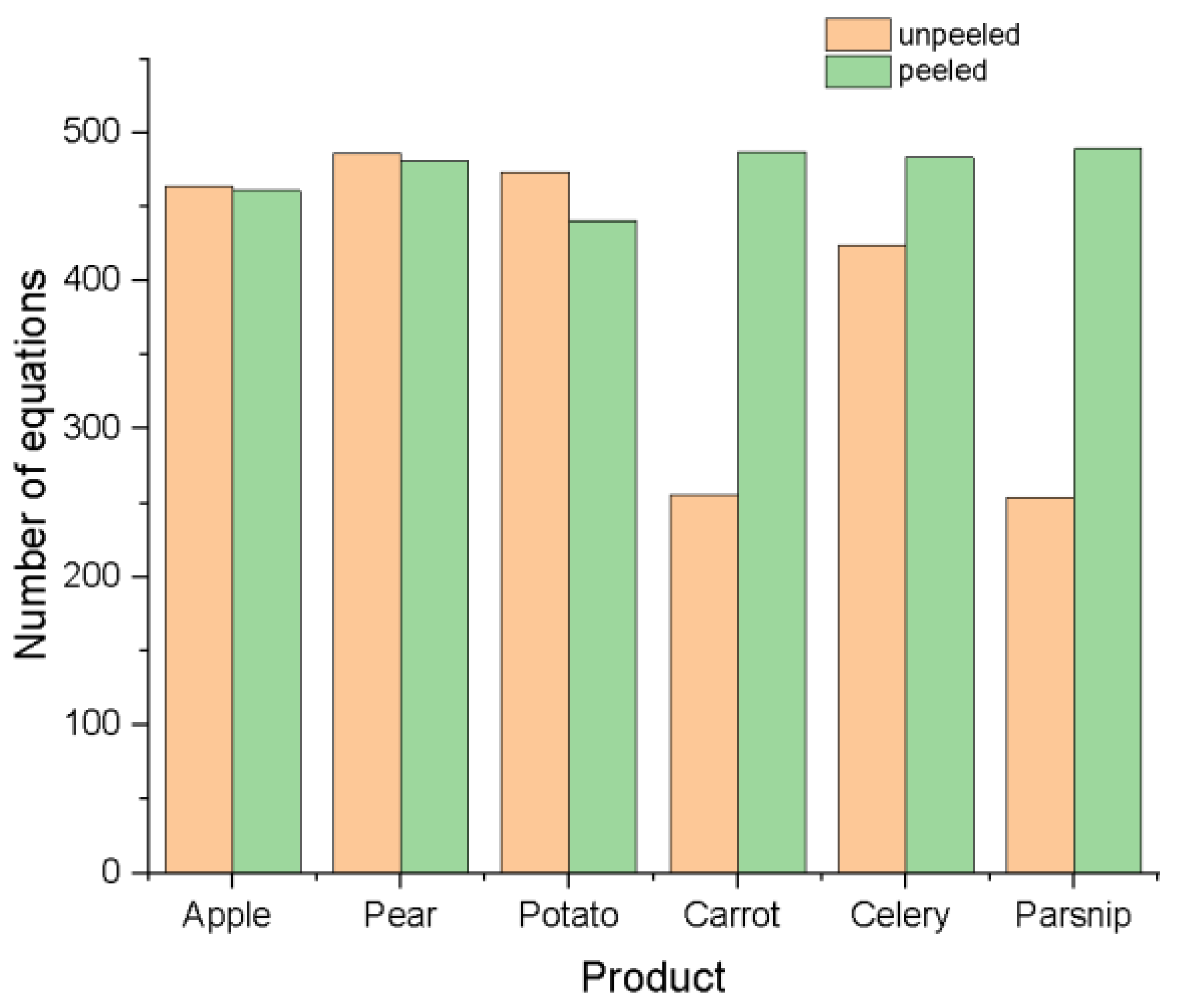
• Following the equations generated by Table Curve 3D software, a total of 5198 equations was generated, which were organized as follows: (Figure 12):

-

2357 for products that have not been peeled;

-

2841 is the number for peeled products.

Table Curve 3D program has a database of these equations, each of which may be recognized by a number, in order to find the common equations.

6.

A selection of common equations has been presented based on this facility, as follows:

-

A number of equations were generated for each group of experiments (with or without a peel) and for each sample in turn (apple, pear, potato, carrot, celery, and parsnip);

-

Within each experimental group (shell products—group a; peeled products—group b), a set of equations with the highest number of equations was chosen in comparison to the equations generated for the other samples (in our situation, we selected 486 equations for group A to correspond to the pear product and 489 equations for group B to correspond to the parsnip product;

-

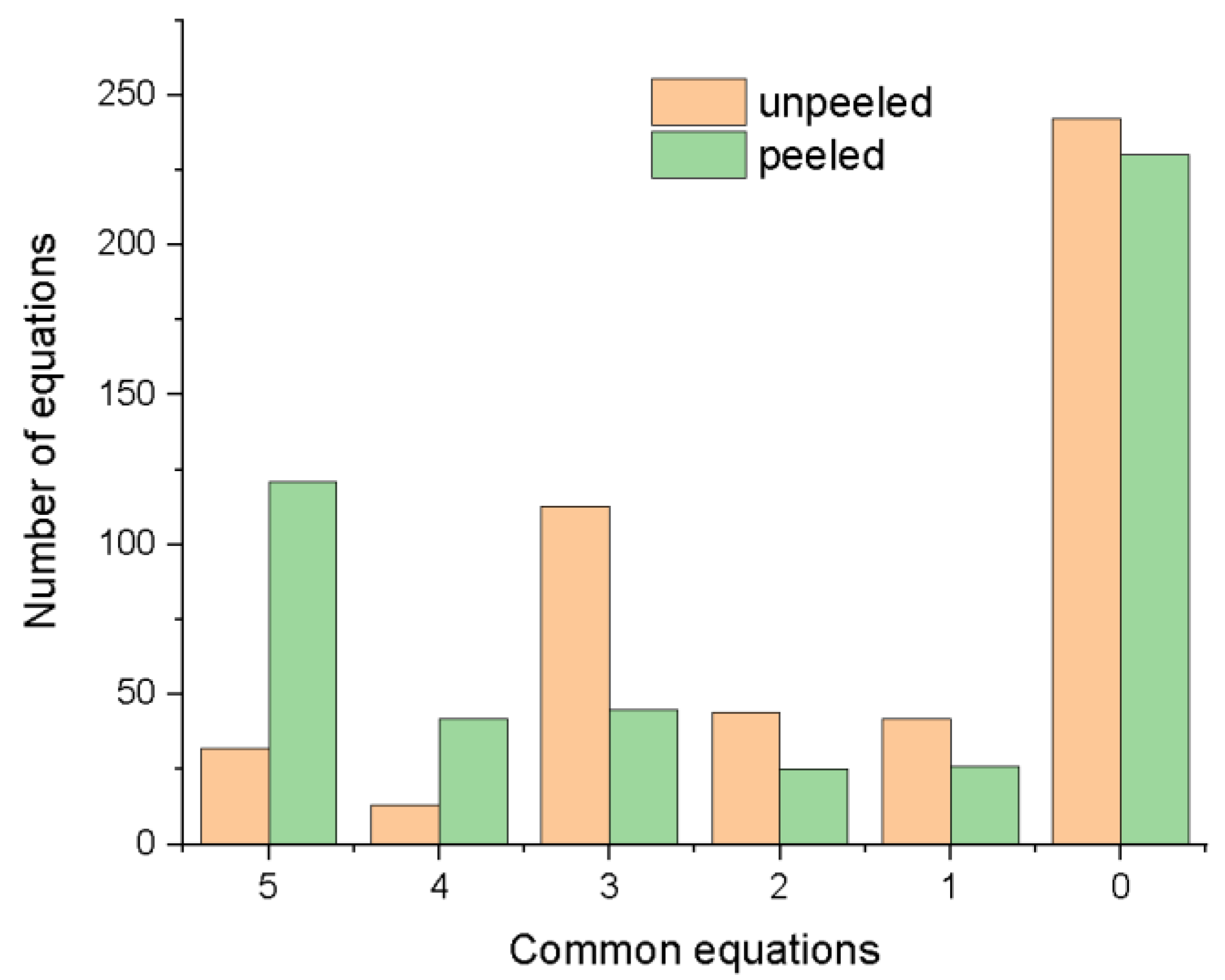
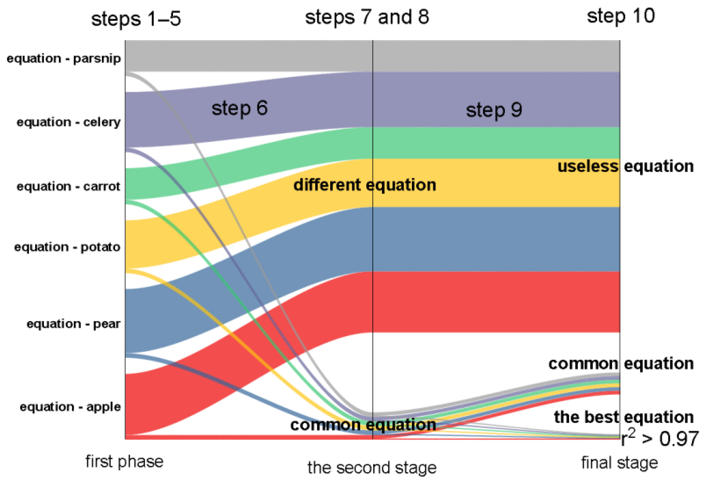
In relation to this lot, similar equations (i.e., equations with the same identification number) have been identified, providing for preliminary filtering of the equations. The number of similar equations obtained from the study is shown in Figure 13. The number of similar equations identified in relation to the equations of the chosen reference lot is represented by numbers such as 5, 4, 3, 2, 1, and 0. (the lot with the most equations) (5—the equation is the same for all products; 0—the equation is unique to each product).

7.

Figure 13 shows the common equations, which are defined by distinct correlation coefficients, and are seen in Figure 14 and Figure 15 for each experimental sample. From the analysis of the graphical representations, it can be said:

-

for unpeeled products, the number of common equations was 32;

-

for peeled products, the number of common equations was 121;

-

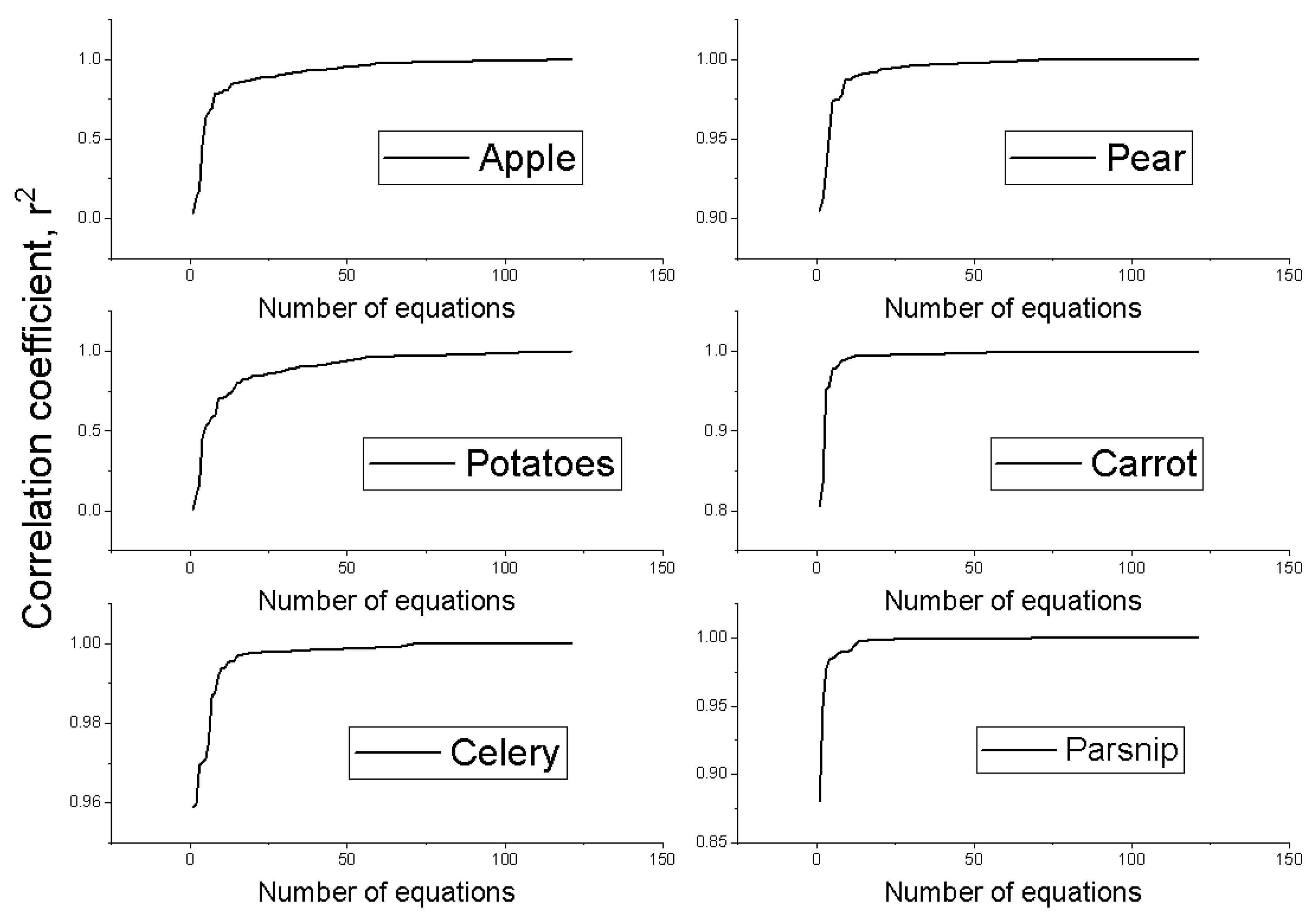
Analyzing the distribution of the number of equations whose correlation coefficient is greater than 0.95 reveals:

-

In the case of unpeeled products, the highest number of equations was obtained for celery (32), followed by pear, parsnip, carrot, and apple, and the lowest number of equations was obtained for potato;

-

In the case of peeled products, the highest number of equations was obtained for celery (121), followed by parsnip, carrot, pear, and apple, and the lowest number of equations was obtained for potato.

8.

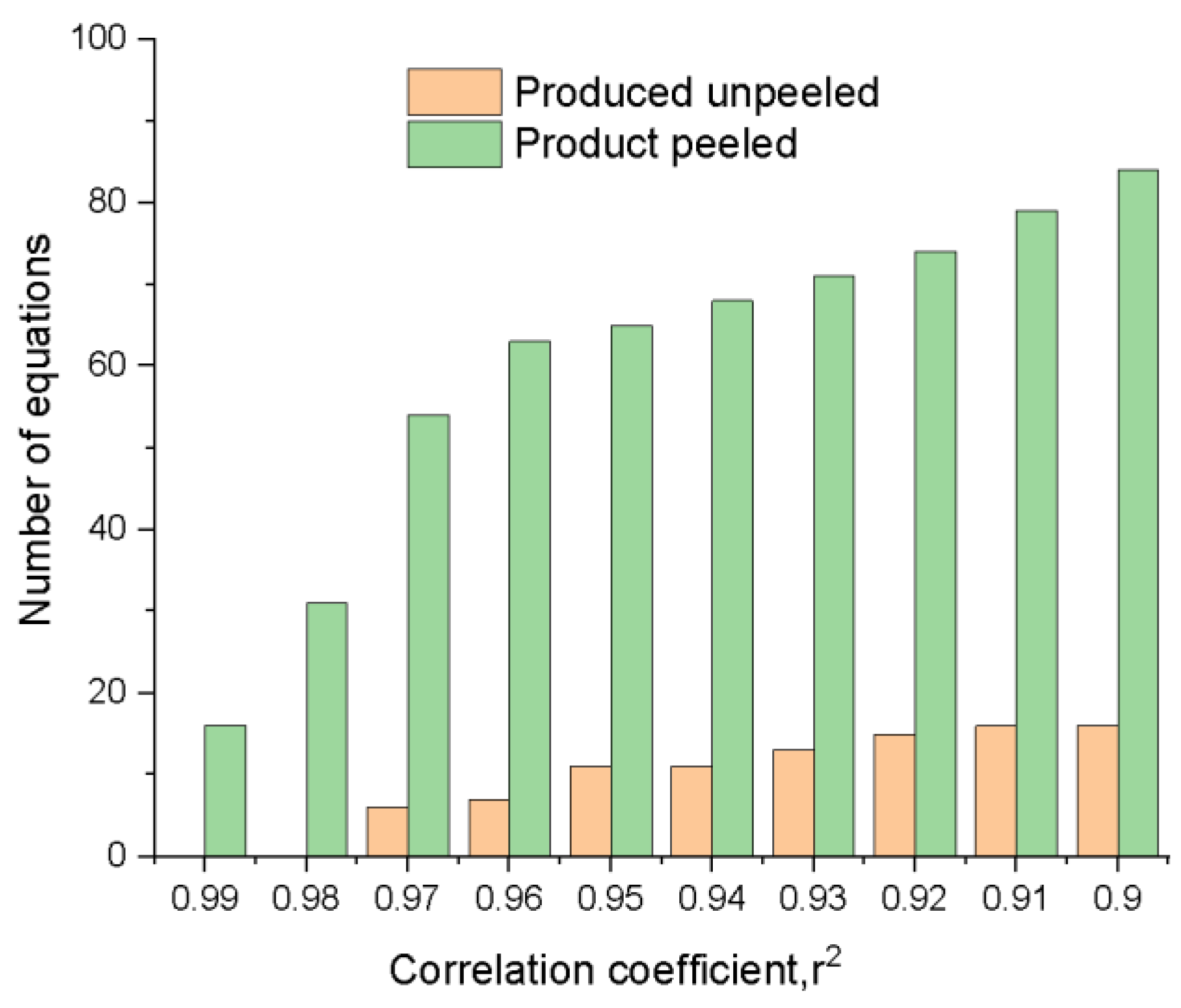
As previously stated, our goal was to find a common equation, therefore we searched over the results more than once to identify the equations with the correlation coefficient, r², which were closest to 0.99. In conclusion, for the range of values of the correlation coefficient r² between 0.9 and 0.99, the number of equations available for solving the desired requirement has been graphically represented in Figure 16.

9.

The evaluation of a group of common equations based on the value of the correlation coefficient r² has been the next step. At this moment, the common equations were created to have the same correlation coefficient value. Followed by an analysis of the correlation coefficients corresponding to the common equations, a total of 6 equations for an r² high of 0.97 have been discovered for the experimental batches of peeled products, and a number of 54 equations for the experimental group of unpeeled products.

The goal of this study was to find the common equations that describe the cutting process for diverse materials for both peeled and unpeeled products. The remaining equations (6 equations for peeled products and 54 equations for unpeeled products) were then analyzed for this purpose, revealing 4 main equations. These four final equations are put through a visual inspection, with the value of the terms of the equations compared to the described equations. This is required if indeed the mathematical model chosen has to be confirmed.

10.

When the values of the terms of the equation generated by the Table Curve 3D software are examined, it is discovered that some equation terms have a value bigger than e⁺⁸, meaning a thorough identification of the relevant term is difficult (since the entire value of the terms is necessary for the validation of the model). Following such an examination, only two possible equations remained out of the four common equations, whose model, in our situation, is provided by the logarithmic equations shown in Equations (3) and (4) (corresponding to equation number 145 and equation number 150—from the Table Curve 3D software database).

$$\begin{array}{c}z=a+b·lnx+c·{\left(lnx\right)}^2+d·{\left(lnx\right)}^3+e·{\left(lnx\right)}^4+f·{\left(lnx\right)}^5+g·lny+h\\ ·{\left(lny\right)}^2+i·{\left(lny\right)}^3+j·{\left(lny\right)}^4+k·{\left(lny\right)}^5\end{array}$$

(3)

$$\begin{array}{c}z=a+b·lnx+c·{\left(lnx\right)}^2+d·{\left(lnx\right)}^3+e·{\left(lnx\right)}^4+f·{\left(lnx\right)}^5+\frac{g}{y}+\frac{h}{y^2}+\frac{i}{y^3}\\ +\frac{j}{y^4}+\frac{k}{y^5}\end{array}$$

(4)

After analyzing the work steps presented above, a graphical representation (Figure 17) was created to highlight the methodology for identifying a general equation to determine the energy required to cut different agri-food products, depending on the speed of the cutting device and the force used to carry out this process. Figure 17 shows the whole methodology for choosing the mathematical equation that explains this procedure, and it is valid for peeled products that have been subjected to experimental determinations (for unpeeled products, the representation is approximately identical).

Figure 18 illustrates the response area created by the Table Curve 3D software in the example of the peeled apple product for equation no. 145.

5. Conclusions

The following conclusions may be taken from the examination of the obtained data:

-

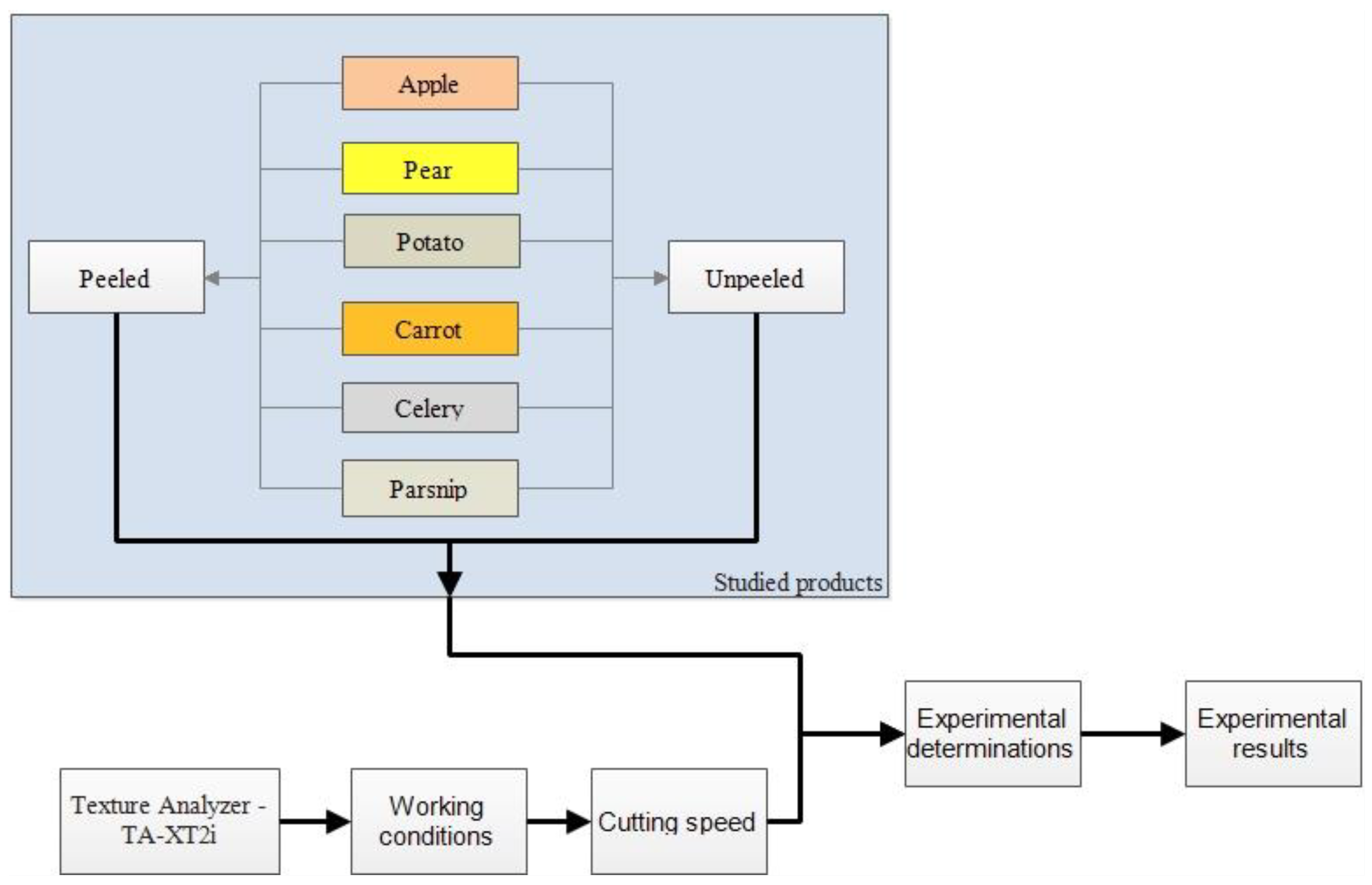
A number of agri-food products (fruit-apple, pear; root-potato, carrot, celery, and parsnip), peeled or unshelled, were used to determine the energy required for cutting vegetable products;

-

Only the density and humidity of the products used could be noted because of the diversity of the chosen products. Taking it into account, the apple has the lowest density (790 kg/m³), while the potato has the highest density (1060 kg/m³). When it regards humidity, potatoes have the lowest humidity (74.5%), and parsnips have the highest (89.5%);

-

The cutting process is influenced directly by the textural properties of the products used in these experimental evaluations:

-

The highest value of energy used to carry out the cutting process was obtained for the product with the lowest humidity, the peeled potato, whose humidity was 74.5% and 23.16 J, respectively, and the lowest value was obtained for unpeeled celery, respectively 11.44 J.

-

In regard to the humidity characteristic, it can be said that it has a direct and inversely proportional influence on the cutting energy value;

-

In terms of product character, both peeled and unpeeled, it is discovered that the energy required to cut peeled products is more than the energy necessary to cut unpeeled products, regardless of the type of the product used;

-

When the energy required to carry out the cutting process is examined in relation to the force used and the cutting device’s speed of movement, it is discovered that these characteristics have a direct impact on the parameter analyzed, independently of the type of the product used;

-

Using the Table Curve 3D software, the obtained data were utilized to produce mathematical equations;

-

An analysis methodology has been developed to identify a common equation for all experimental groups, which can be generalized to other types of experiments as well;

-

Following the working stages of the experimental data, it is found that:

-

For peeled products, where a total of 2357 equations were created, 32 common equations were generated, only 6 of which satisfied the criterion of r² being larger than 0.97;

-

For unpeeled products, it resulted in a total of 2841 equations, 121 of which were common and 54 of which satisfied the requirement of r² having larger than 0.97;

-

Following a visual examination of the Table Curve 3D program’s mathematical equations, which satisfied the two primary requirements:

○

To have an r²> of 0.97 (6 equations for peeled products and 54 for unpeeled products);

○

To have something in common with both peeled and unpeeled products;

○

We had the option of choosing between two logarithmic equations;

-

Two common logarithmic equations describing the dependency between the cutting energy required to cut different types of products (peeled and/or unpeeled) depending on the cutting speed and force, and the dependency characteristic of the cutting process of hard-textured products, were identified following the analysis of the equations obtained using the Table Curve 3D software.

References

- Earle, R.L. Unit Operations in Food Industry; The New Zealand Institute of Food Science and Technology: Palmerston North, New Zealand, 1983. [Google Scholar]
- Mohsenin, N.N. Physical Properties of Plant and Animal Materials; Gordon and Breach Science Publishers: New York, NY, USA, 1970. [Google Scholar]
- Bourne, M.C. Basic Principles of Food Texture Measurement; Lecture text of Dough Rheology and Baked Products Texture Workshop: Chicago, IL, USA, 1988. [Google Scholar]
- Mani, S.; Tabil, L.G.; Sokhansanj, S. Grinding performance and physical properties of wheat and barley straws, corn stover and switchgrass. Biomass Bioenergy 2004, 27, 339–352. [Google Scholar] [CrossRef]
- Tumuluru, J.S.; Tabil, L.G.; Song, Y.; Iroba, K.L.; Meda, V. Grinding energy and physical properties of chopped and hammer-milled barley, wheat, oat, and canola straws. Biomass Bioenergy 2014, 60, 58–67. [Google Scholar] [CrossRef]
- Liu, Y.; Wang, J.; Wolcott, M.P. Assessing the specific energy consumption and physical properties of comminuted Douglas-fir chips for bioconversion. Ind. Crops Prod. 2016, 94, 394–400. [Google Scholar] [CrossRef]
- Panainte, M.; Nedeff, V.; Burcă, G.; Savin, C.; Mosnegutu, E. Theoretical consideration regarding statistical calculus about distribution of size at particles at result from grinding process. MOCM 2004, 10, 83–88. [Google Scholar]
- Cadoche, L.; Lopez, G.D. Assessment of size-reduction as a preliminary step in the production of ethanol from lignocellulosic wastes. Biol. Wastes 1989, 30, 153–157. [Google Scholar] [CrossRef]
- Panainte, M.; Nedeff, V.; Moşneguţu, E. Analysis of grinding process at hammer mill. MOCM 2001, 7, 120–129. [Google Scholar]
- Panainte, M.; Dasic, P.; Nedeff, V.; Mosnegutu, E.; Savin, C. Modalities to determine the energy consomption for the grindin gat vegetables product with variable texture. MOCM 2007, 13, 239–248. [Google Scholar]
- Brennan, J.G. Food texture measurement. In Developments in Food Analysis Techniques; Elsevier Applied Science Publishers: London, UK, 1980; Volume 2. [Google Scholar]
- Ragni, L.; Berardinelli, A. Mechanical behaviour of apples and damage during sorting a packaging. J. Agric. Engng. Res. 2001, 78, 78–91. [Google Scholar]
- Panainte, M.; Nedeff, V.; Moşneguţu, E.; Savin, C.; Măcărescu, B.; Olaru, C. Determination of grinding energy to vegetable product through texture analysis method. MOCM 2007, 3, 128–134. [Google Scholar]
- Adapa, P.; Tabil, L.; Schoenau, G. Grinding performance and physical properties of non-treated and steam exploded barley, canola, oat and wheat straw. Biomass Bioenergy 2011, 35, 549–561. [Google Scholar] [CrossRef]
- Naimi, L.J.; Sokhansanj, S.; Bi, X.; Lim, C.J.; Womac, A.R.; Lau, A.K.; Melin, S. Development of size reduction equations for calculating energy input for grinding lignocellulosic particles. Appl. Eng. Agric. 2013, 29, 93–100. [Google Scholar] [CrossRef]
- Karam, M.C.; Petit, J.; Zimmer, D.; Djantou, E.B.; Scher, J. Effects of drying and grinding in production of fruit and vegetable powders: A review. J. Food Eng. 2016, 188, 32–49. [Google Scholar] [CrossRef]
- Indira, T.N.; Bhattacharya, S. Grinding characteristics of some legumes. J. Food Eng. 2006, 76, 113–118. [Google Scholar] [CrossRef]
- Xiaoan, L.; Qinghong, L.; Fan, G.; Cong, H.; Peng, J.; Yonghua, Z. Effect of cutting styles on quality and antioxidant activity in fresh-cut pitaya fruit. Postharvest Biol. Technol. 2017, 124, 1–7. [Google Scholar]
- Bitra, V.S.P.; Womac, A.R.; Chevanan, N.; Miu, P.I.; Igathinathane, C.; Sokhansanj, S.; Smith, D.R. Direct mechanical energy measures of hammer mill comminution of switchgrass, wheat straw, and corn stover and analysis of their particle size distributions. Powder Technol. 2009, 193, 32–45. [Google Scholar] [CrossRef]
- Kratky, L.; Jirout, T. Modelling of particle size characteristics and specific energy demand for mechanical size reduction of wheat straw by knife mill. Biosyst. Eng. 2022, 197, 32–44. [Google Scholar] [CrossRef]
- Panainte, M.; Moşneguţu, E.; Savin, C.; Nedeff, V. Mărunţirea Produselor Agroalimentare; Meronia, Rovimed Publishers: Bacău, Romania, 2005. [Google Scholar]
- Panainte, M. Researches Regarding Optimizing the Grinding Process of Agrofood Products. Ph.D. Thesis, The “Gheorghe Asachi” Technical University of Iasi, Iași, Romania, 2008. [Google Scholar]
- Ladan, J.N.; Shahab, S. Data-based equation to predict power and energy input for grinding wheat straw, corn stover, switchgrass, miscanthus, and canola straw. Fuel Process. Technol. 2018, 173, 81–88. [Google Scholar]
- Wang, Y.L.J.; Barth, J.C.; Welsch, K.R.; McIntyre, V.; Wolcot, M.P. Effects of multi-stage milling method on the energy consumption of comminuting forest residuals. Ind. Crops Prod. 2022, 145, 111955. [Google Scholar]
- Flumignan, D.L.; Rezende, K.A.; Comunello, E.M.; Fietz, C.R. Empirical methods for estimating reference surface net radiation from solar radiation. Eng. Agrícola 2018, 38, 32–37. [Google Scholar] [CrossRef]
- Saruchi, S.A.; Ariff, M.H.M.; Zamzuri, H.; Hassan, N.; Nurbaiti, W. Artificial neural network for modelling of the correlation between lateral acceleration and head movement in a motion sickness study. IET Intell. Transp. Syst. 2018, 13, 340–346. [Google Scholar] [CrossRef]
- Paterson, C.; Clevers, H.; Bozic, I. Mathematical model of colorectal cancer initiation. Proc. Natl. Acad. Sci. USA 2022, 117, 20681–20688. [Google Scholar] [CrossRef] [PubMed]
- Watanabe, S.; Kitawaki, T.; Oka, H. Mathematical equation of fusion index of tetanic contraction of skeletal muscles. J. Electromyogr. Kinesiol. 2010, 20, 284–289. [Google Scholar] [CrossRef] [PubMed]
- Yu, Y.; Liu, J.X.; Zhang, K. Establishment of a prediction model for the cut size of turbo air classifiers. Powder Technol. 2014, 254, 274–280. [Google Scholar] [CrossRef]
- Ageev, A.A.; Yakhontov, D.A.; Kadyrov, T.F.; Farakhov, M.M.; Lapteva, E.A. Mathematical equation of dispersed phase gas separation in a combined equipment. Chem. Petrol. Eng 2019, 55, 611–618. [Google Scholar] [CrossRef]
- Hwang, D.H.; Han, J.H.; Lee, J.; Lee, Y.; Kim, D. A mathematical equation for the separation behavior of a split type low-shock separation bolt. Acta Astronaut. 2019, 164, 393–406. [Google Scholar] [CrossRef]
- Ibyatov, R.I.; Kholpanov, L.P.; Akhmadiev, F.G.; Fazylzyanov, R.R. Mathematical modeling of phase separation of a multiphase medium. Theor. Found. Chem. Eng. 2006, 40, 339–348. [Google Scholar] [CrossRef]
- Song, J.F.; Hu, X.F. A mathematical equation to calculate the separation efficiency of streamlined plate gas-liquid separator. Sep. Purif. Technol. 2017, 178, 242–252. [Google Scholar] [CrossRef]
- Cobzaru, C.; Marinoiu, A.; Apostolescu, G.A.; Tataru-Farmus, R.E.; Cernatescu, C. Mathematical modeling for kinetics of Fe3+ exchange on pretreated analcime. Rev. Roum. De Chim. 2019, 64, 403–407. [Google Scholar] [CrossRef]
- Mosnegutu, E.; Panainte-Lehadus, M.; Nedeff, V.; Tomozei, C.; Barsan, N.; Chitimus, D.; Jasinski, M. Extraction of mathematical correlations applied in the aerodynamic separation of solid particles. Processes 2022, 10, 1234. [Google Scholar] [CrossRef]
- Xxx, Stable Micro Systems. Available online: https://www.stablemicrosystems.com (accessed on 13 March 2020).
- SYSTAT Software Inc. TableCurve 3D, Version 4.0. Available online: https://systatsoftware.com/downloads/download-tablecurve-3d/ (accessed on 13 March 2020).