Modelling Deaggregation Due to Normal Carrier–Wall Collision in Dry Powder Inhalers

 ,
,  ,
, 

Abstract
:1. Introduction
2. Materials and Methods
DEM Approach
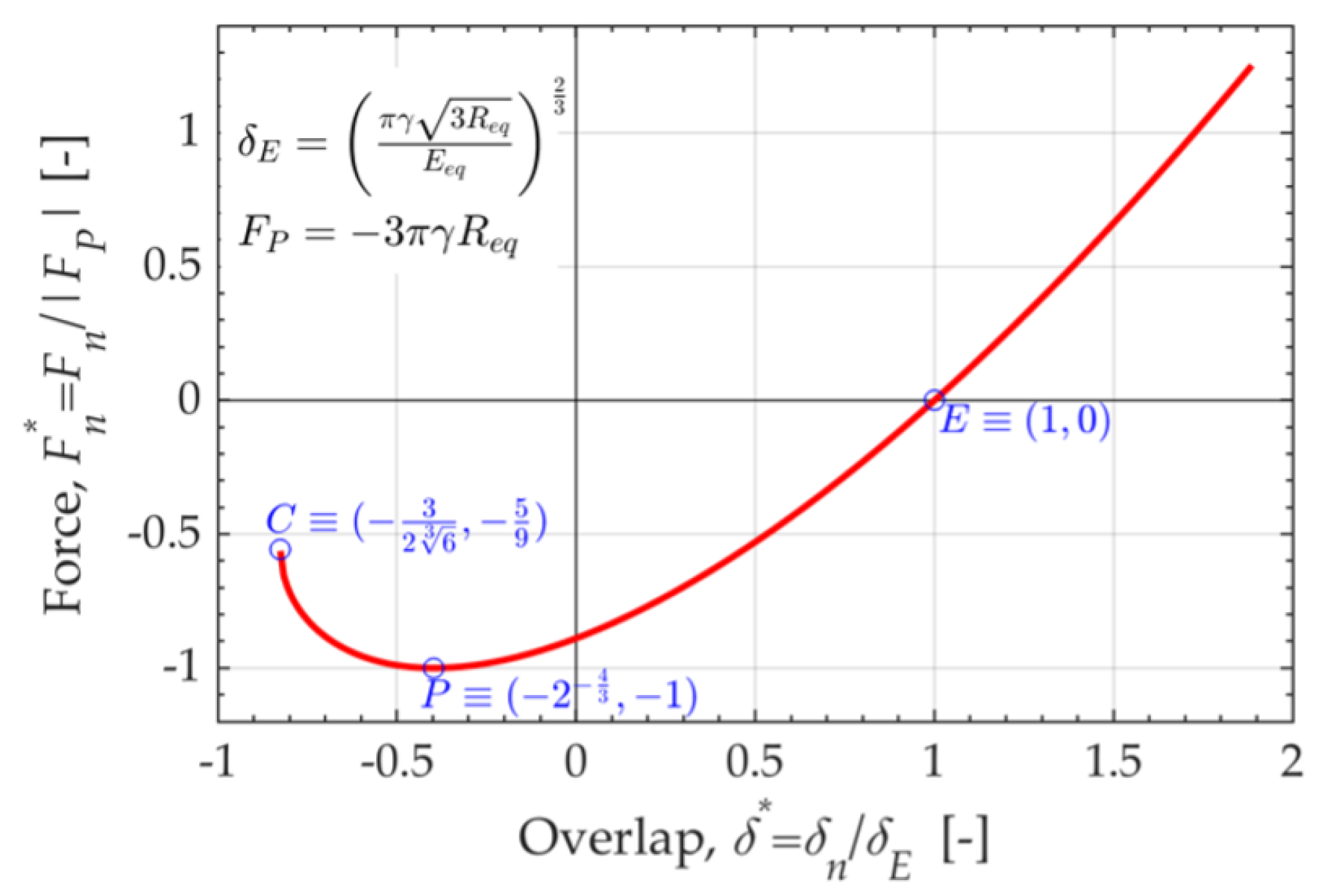
Cohesion Models
3. DEM Model of the Detachment Process
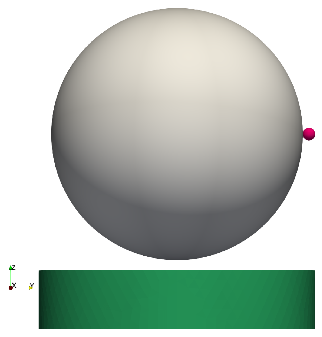
3.1. Simulation Set-Up and Parameters
3.2. Escape Velocity
3.3. Influence of Dissipation Parameters
3.4. The Role of Rolling Friction
4. Analytical Model for the Escape Velocity
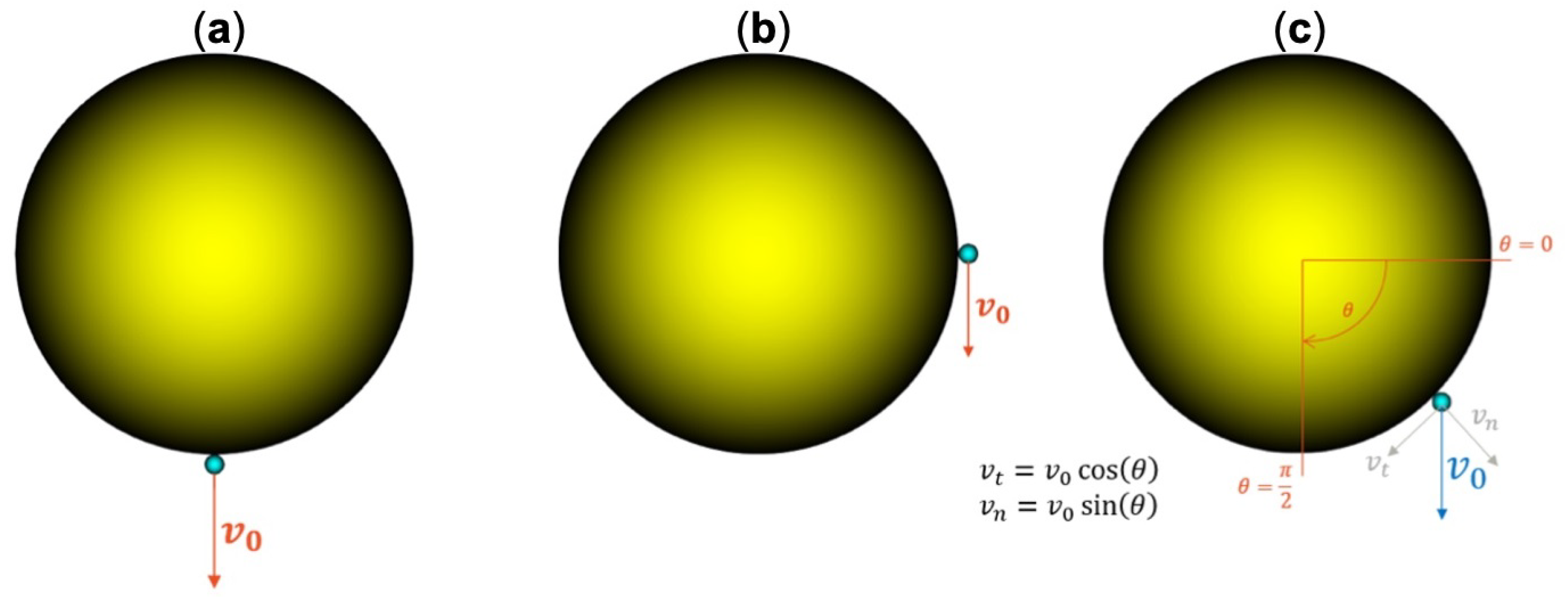
4.1. South Pole Detachment
4.2. Equatorial Detachment
4.3. General South-Hemisphere Detachment
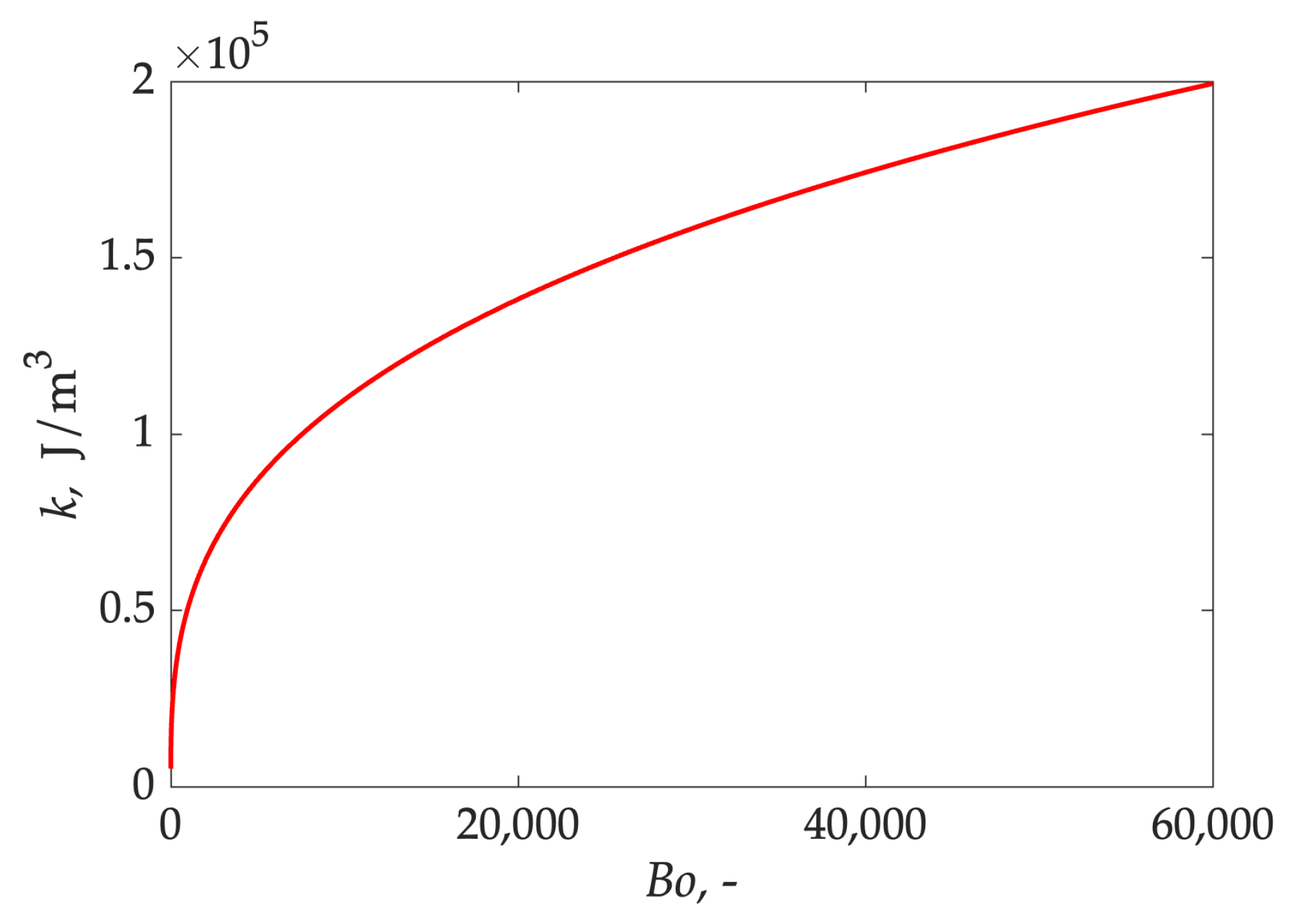
4.4. Calculation of Cohesion Energy
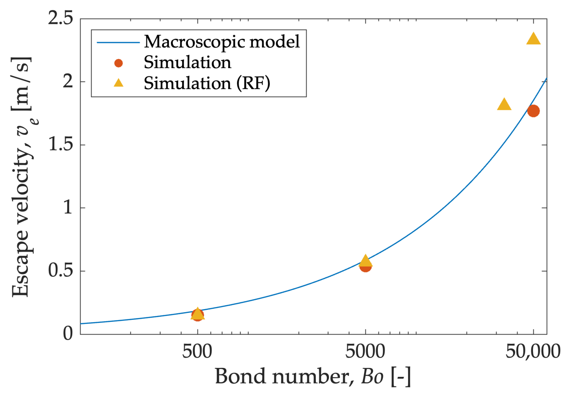
4.5. Comparison with DEM Simulations
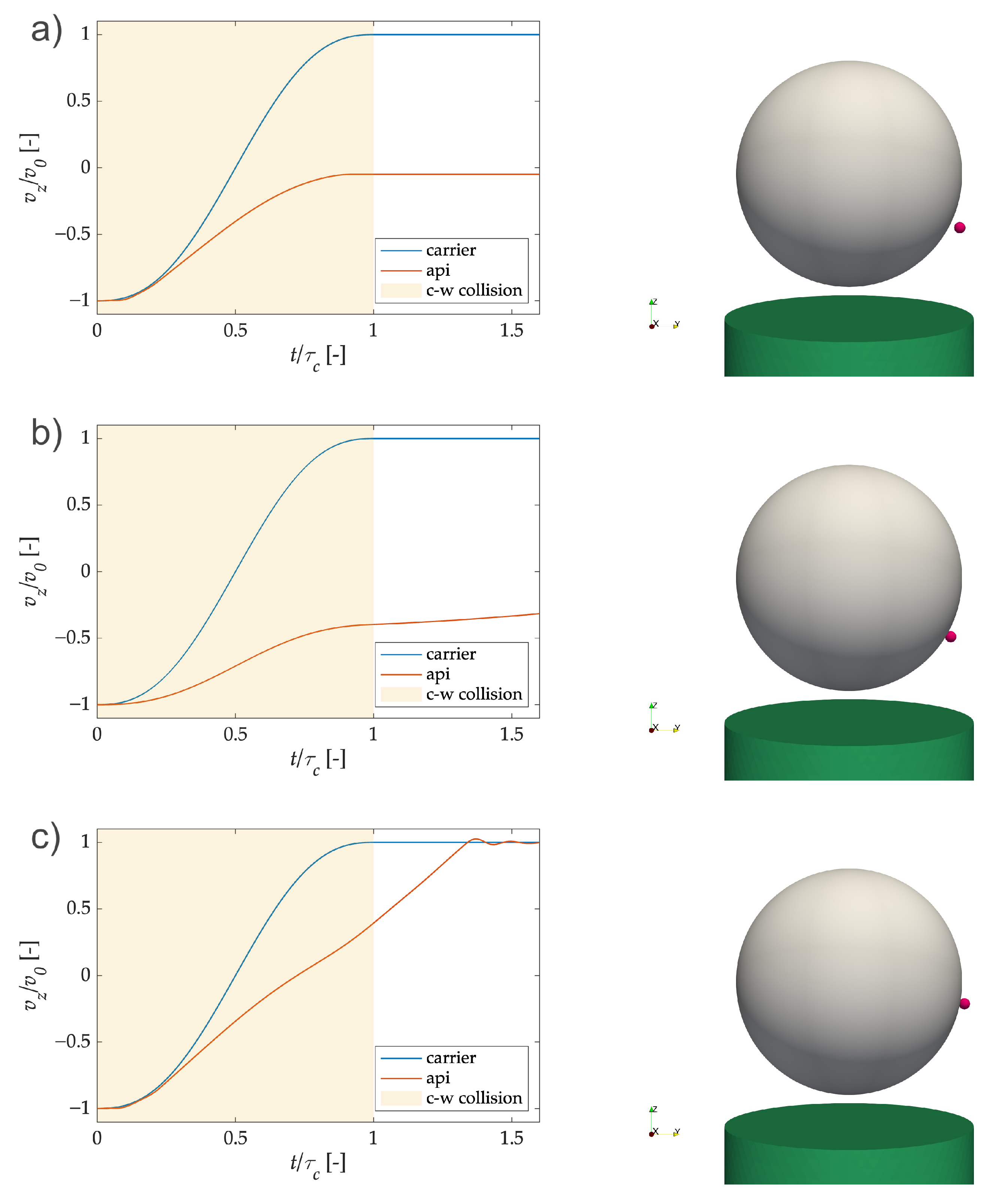
4.6. Effect of the Carrier–Wall Collision Dynamics
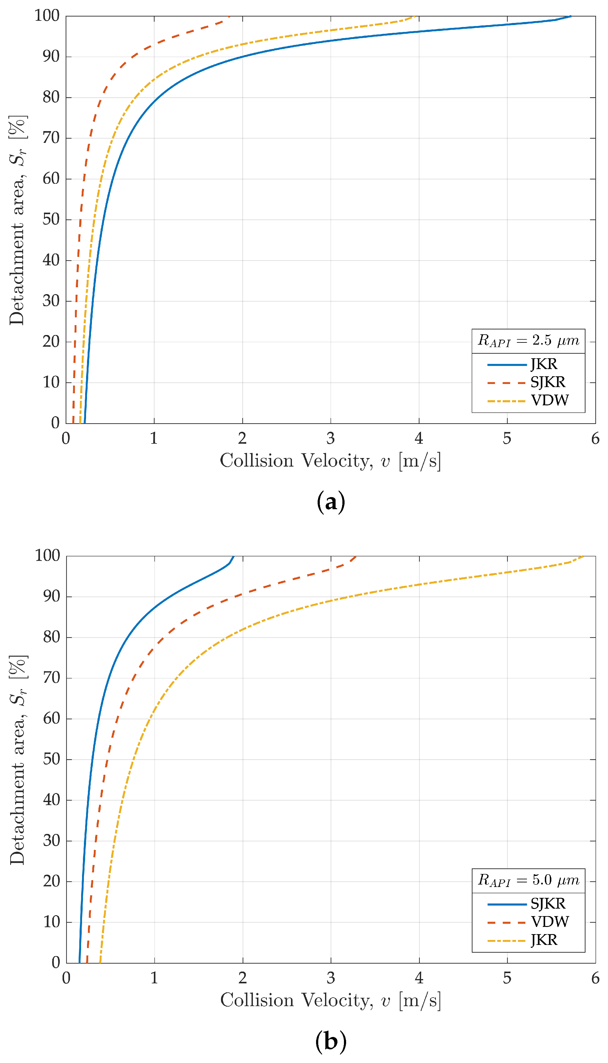
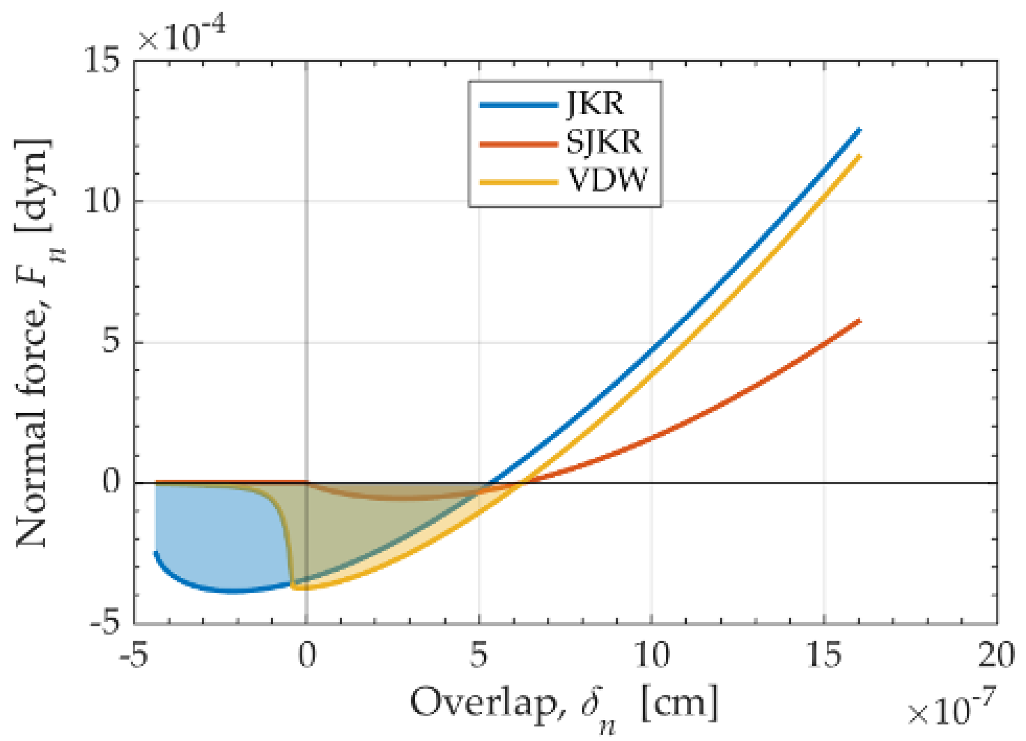
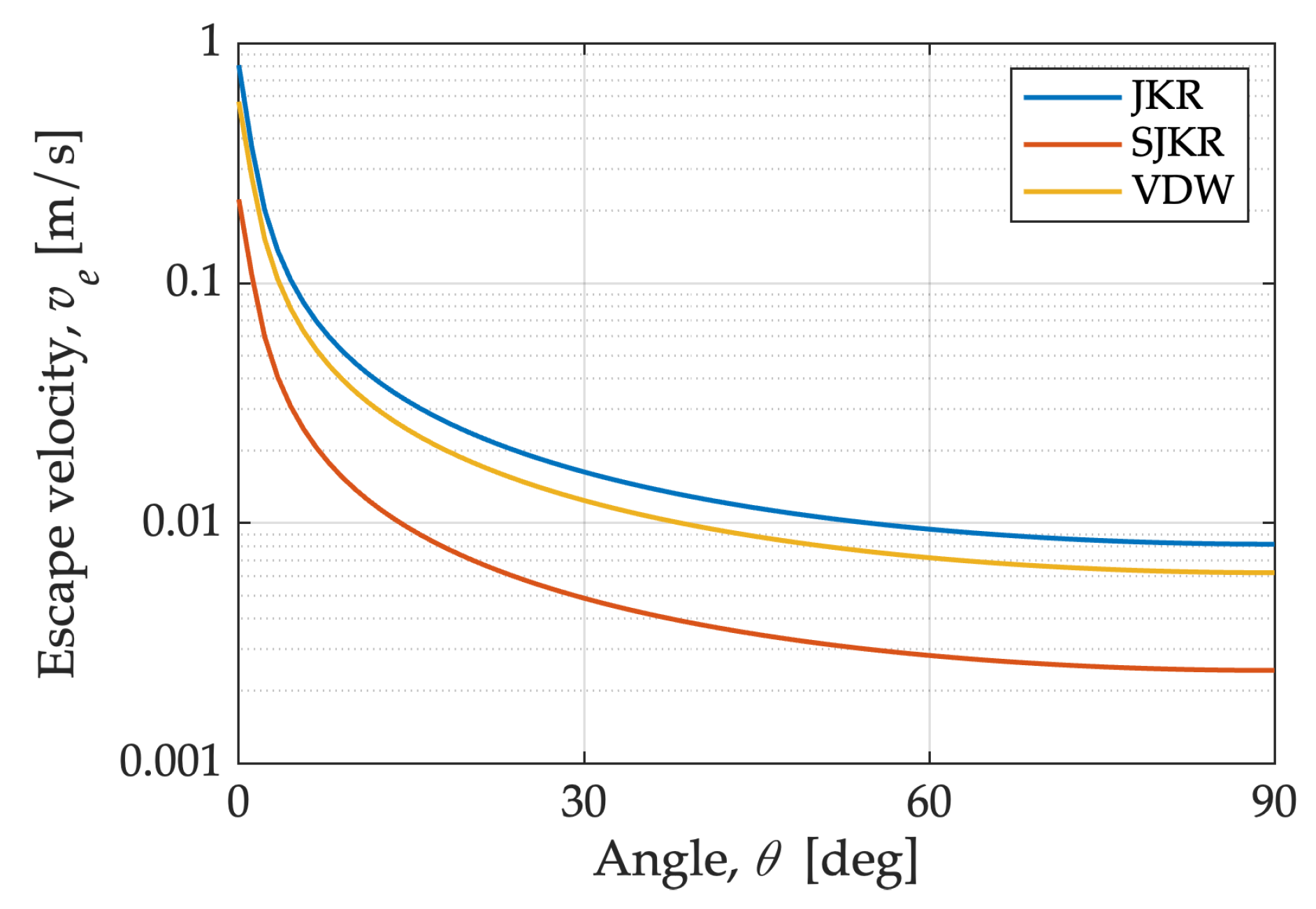
4.7. Effect of the Cohesion Model on Escape Velocity
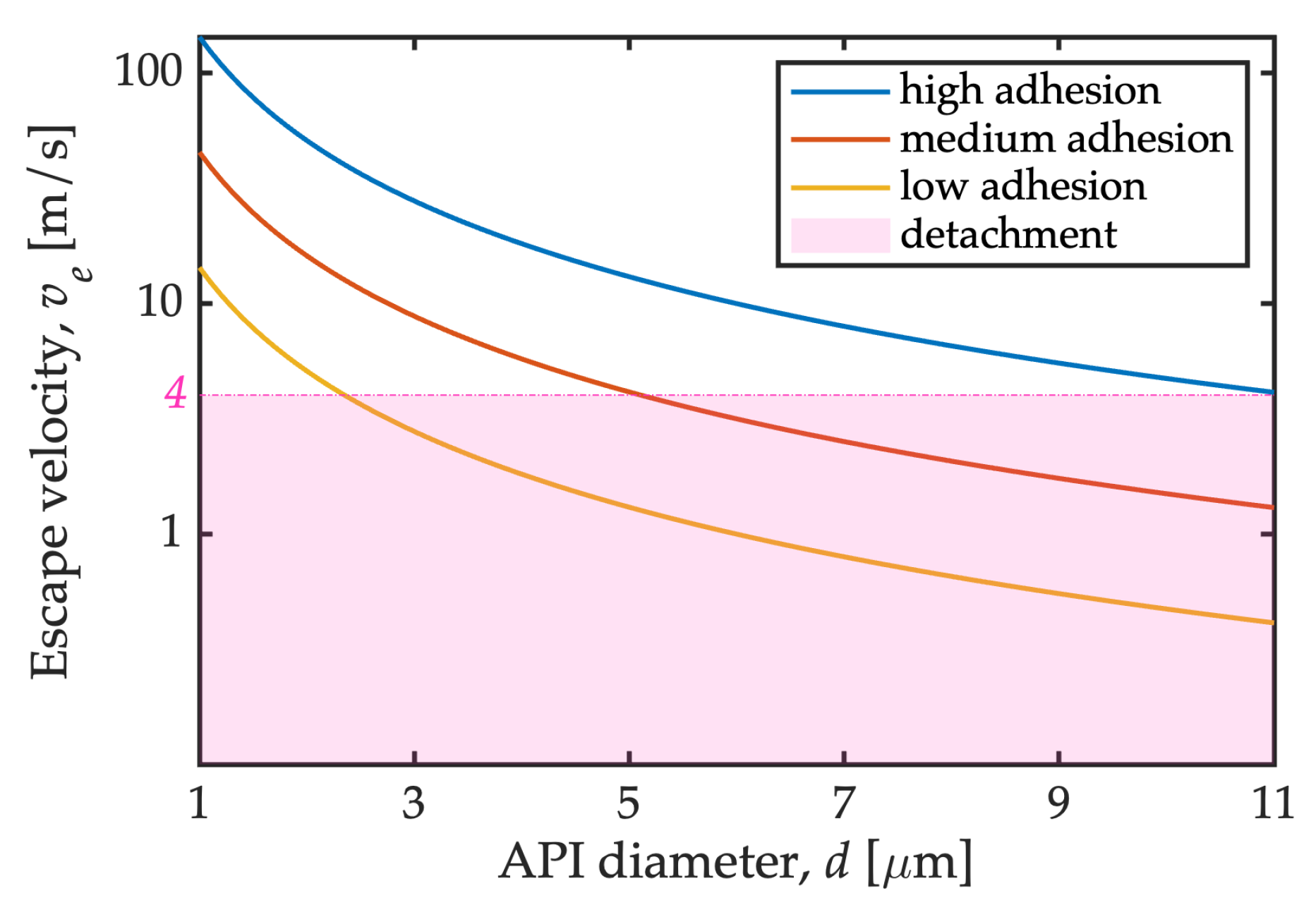
4.8. Relation with Actual Deaggregation Conditions
5. Conclusions
Author Contributions
Funding
Institutional Review Board Statement
Informed Consent Statement
Data Availability Statement
Conflicts of Interest
Abbreviations
| API | Active Pharmaceutical Ingredient |
| DPI | Dry Powder Inhaler |
| JKR | Johnson–Kendall–Roberts contact model |
| SJKR | Linear cohesion model |
| VDW | Constant cohesion model |
| CDT | Constant Directional Torque rolling friction model |
| AFM | Atomic force microscopy |
| RF | Rolling friction |
| PP | Particle–particle |
| PW | Particle–wall |
Nomenclature
| Position vector of particle i | |
| Velocity vector of particle i | |
| Angular velocity vector of particle i | |
| Number of particles i | |
| Total force | |
| Contact force | |
| Cohesion force | |
| Drag force | |
| Pressure gradient force | |
| Lift force | |
| Gravity force | |
| Total torque | |
| Contact torque | |
| Rolling resistance torque | |
| Equivalent Young modulus | |
| Equivalent shear modulus | |
| Equivalent radius | |
| Normal overlap | |
| Tangential overlap | |
| Normal impact velocity | |
| Tangential impact velocity | |
| Normal damping coefficient | |
| Tangential damping coefficient | |
| Static friction coefficient | |
| Rolling friction coefficient | |
| a | Radius of the contact area |
| Contact area | |
| Cohesion surface energy (JKR, VDW models) | |
| k | Cohesion energy density (SJKR model) |
| Inner cutoff for cohesive forces | |
| Outer cutoff for cohesive forces | |
| m | Particle mass |
| R | Particle radius |
| Density | |
| E | Young modulus |
| ∋ | Poisson coefficient |
| e | Coefficient of restitution |
| Bond number | |
| Equilibrium force | |
| Equilibrium overlap (normal) | |
| Escape velocity | |
| Kinetic energy | |
| Cohesion energy | |
| Centrifugal force | |
| Work of the centrifugal force | |
| API angular position on carrier |
Appendix A. Conversion of Translational Energy

Appendix B. Cohesion Energy
Appendix B.1. SJKR Model
Appendix B.2. JKR Model
Appendix B.3. VDW Model

Appendix C. Additional Relationships for the Escape Velocity
Appendix C.1. Derivation of Cohesion Model Parameters
Appendix C.1.1. SJKR Model
Appendix C.1.2. JKR Model
Appendix C.1.3. VDW Model
Appendix C.2. Equatorial Velocity (0°)
Appendix C.3. South Pole Velocity (90°)
Appendix C.4. Velocity Ratio
Appendix C.5. General South-Hemisphere Detachment
Appendix C.6. Alternative Relationships
References
- Hoppentocht, M.; Hagedoorn, P.; Frijlink, H.; De Boer, A. Technological and practical challenges of Dry Powder Inhalers and formulations. Adv. Drug Deliv. Rev. 2014, 75, 18–31. [Google Scholar] [CrossRef] [PubMed] [Green Version]
- Rashid, M.A.; Muneer, S.; Mendhi, J.; Sabuj, M.Z.R.; Alhamhoom, Y.; Xiao, Y.; Wang, T.; Izake, E.L.; Islam, N. Inhaled Edoxaban dry powder inhaler formulations: Development, characterization and their effects on the coagulopathy associated with COVID-19 infection. Int. J. Pharm. 2021, 608, 121122. [Google Scholar] [CrossRef] [PubMed]
- Sommerfeld, M.; Cui, Y.; Schmalfuß, S. Potential and constraints for the application of CFD combined with Lagrangian particle tracking to Dry Powder Inhalers. Eur. J. Pharm. Sci. 2019, 128, 299–324. [Google Scholar] [CrossRef]
- Begat, P.; Morton, D.A.; Staniforth, J.N.; Price, R. The cohesive-adhesive balances in dry powder inhaler formulations I: Direct quantification by atomic force microscopy. Pharm. Res. 2004, 21, 1591–1597. [Google Scholar] [CrossRef] [PubMed]
- Zafar, U.; Alfano, F.; Ghadiri, M. Evaluation of a new dispersion technique for assessing triboelectric charging of powders. Int. J. Pharm. 2018, 543, 151–159. [Google Scholar] [CrossRef]
- Alfano, F.O.; Di Renzo, A.; Di Maio, F.P.; Ghadiri, M. Computational analysis of triboelectrification due to aerodynamic powder dispersion. Powder Technol. 2021, 382, 491–504. [Google Scholar] [CrossRef]
- Finlay, W.H. The Mechanics of Inhaled Pharmaceutical Aerosols: An Introduction; Academic Press: London, UK, 2001. [Google Scholar]
- Cavalli, G.; Bosi, R.; Ghiretti, A.; Cottini, C.; Benassi, A.; Gaspari, R. A shear cell study on oral and inhalation grade lactose powders. Powder Technol. 2020, 372, 117–127. [Google Scholar] [CrossRef]
- de Boer, A.H.; Hagedoorn, P.; Hoppentocht, M.; Buttini, F.; Grasmeijer, F.; Frijlink, H.W. Dry powder inhalation: Past, present and future. Expert Opin. Drug Deliv. 2017, 14, 499–512. [Google Scholar] [CrossRef] [Green Version]
- Dos Reis, L.G.; Chaugule, V.; Fletcher, D.F.; Young, P.M.; Traini, D.; Soria, J. In-vitro and particle image velocimetry studies of dry powder inhalers. Int. J. Pharm. 2021, 592, 119966. [Google Scholar] [CrossRef]
- Pasquali, I.; Merusi, C.; Brambilla, G.; Long, E.J.; Hargrave, G.K.; Versteeg, H.K. Optical diagnostics study of air flow and powder fluidisation in Nexthaler®—Part I: Studies with lactose placebo formulation. Int. J. Pharm. 2015, 496, 780–791. [Google Scholar] [CrossRef] [Green Version]
- Fletcher, D.F.; Chaugule, V.; Gomes dos Reis, L.; Young, P.M.; Traini, D.; Soria, J. On the use of computational fluid dynamics (CFD) modelling to design improved dry powder inhalers. Pharm. Res. 2021, 38, 277–288. [Google Scholar] [CrossRef] [PubMed]
- Merusi, C.; Brambilla, G.; Long, E.; Hargrave, G.; Versteeg, H. Optical diagnostics studies of air flow and powder fluidisation in Nexthaler®. Part II: Use of fluorescent imaging to characterise transient release of fines from a dry powder inhaler. Int. J. Pharm. 2018, 549, 96–108. [Google Scholar] [CrossRef] [PubMed] [Green Version]
- Kou, X.; Wereley, S.T.; Heng, P.W.; Chan, L.W.; Carvajal, M.T. Powder dispersion mechanisms within a dry powder inhaler using microscale particle image velocimetry. Int. J. Pharm. 2016, 514, 445–455. [Google Scholar] [CrossRef] [PubMed]
- Benassi, A.; Cottini, C. Numerical Simulations for Inhalation Product Development: Achievements and Current Limitations. ONdrugDelivery 2021, 127, 68–75. [Google Scholar]
- Ariane, M.; Sommerfeld, M.; Alexiadis, A. Wall collision and drug-carrier detachment in dry powder inhalers: Using DEM to devise a sub-scale model for CFD calculations. Powder Technol. 2018, 334, 65–75. [Google Scholar] [CrossRef]
- Sarangi, S.; Thalberg, K.; Frenning, G. Effect of carrier size and mechanical properties on adhesive unit stability for inhalation: A numerical study. Powder Technol. 2021, 390, 230–239. [Google Scholar] [CrossRef]
- Tamadondar, M.R.; Rasmuson, A. The effect of carrier surface roughness on wall collision-induced detachment of micronized pharmaceutical particles. AIChE J. 2020, 66, e16771. [Google Scholar] [CrossRef]
- Tong, Z.; Kamiya, H.; Yu, A.; Chan, H.K.; Yang, R. Multi-scale modelling of powder dispersion in a carrier-based inhalation system. Pharm. Res. 2015, 32, 2086–2096. [Google Scholar] [CrossRef]
- Schulz, D.; Woschny, N.; Schmidt, E.; Kruggel-Emden, H. Modelling of the detachment of adhesive dust particles during bulk solid particle impact to enhance dust detachment functions. Powder Technol. 2022, 400, 117238. [Google Scholar] [CrossRef]
- Yang, J.; Wu, C.Y.; Adams, M. Three-dimensional DEM–CFD analysis of air-flow-induced detachment of API particles from carrier particles in dry powder inhalers. Acta Pharm. Sin. B 2014, 4, 52–59. [Google Scholar] [CrossRef] [Green Version]
- Alfano, F.O.; Benassi, A.; Gaspari, R.; Di Renzo, A.; Di Maio, F.P. Full-Scale DEM Simulation of Coupled Fluid and Dry-Coated Particle Flow in Swirl-Based Dry Powder Inhalers. Ind. Eng. Chem. Res. 2021, 60, 15310–15326. [Google Scholar] [CrossRef]
- Zhao, J.; Haghnegahdar, A.; Feng, Y.; Patil, A.; Kulkarni, N.; Singh, G.J.P.; Malhotra, G.; Bharadwaj, R. Prediction of the carrier shape effect on particle transport, interaction and deposition in two dry powder inhalers and a mouth-to-G13 human respiratory system: A CFD-DEM study. J. Aerosol Sci. 2022, 160, 105899. [Google Scholar] [CrossRef]
- Tong, Z.; Yang, R.; Yu, A. CFD-DEM study of the aerosolisation mechanism of carrier-based formulations with high drug loadings. Powder Technol. 2017, 314, 620–626. [Google Scholar] [CrossRef]
- Alfano, F.; Di Maio, F.; Di Renzo, A. Deagglomeration of selected high-load API-carrier particles in swirl-based dry powder inhalers. Powder Technol. 2022, 408, 117800. [Google Scholar] [CrossRef]
- Garg, R.; Galvin, J.; Li, T.; Pannala, S. Open-source MFIX-DEM software for gas-solids flows: Part I-Verification studies. Powder Technol. 2012, 220, 122–137. [Google Scholar] [CrossRef]
- Tsuji, Y.; Kawaguchi, T.; Tanaka, T. Discrete particle simulation of two-dimensional fluidized bed. Powder Technol. 1993, 77, 79–87. [Google Scholar] [CrossRef]
- Di Renzo, A.; Di Maio, F. Comparison of contact-force models for the simulation of collisions in DEM-based granular flow codes. Chem. Eng. Sci. 2004, 59, 525–541. [Google Scholar] [CrossRef]
- Ai, J.; Chen, J.F.; Rotter, J.; Ooi, J. Assessment of rolling resistance models in discrete element simulations. Powder Technol. 2011, 206, 269–282. [Google Scholar] [CrossRef]
- Johnson, K.L.; Kendall, K.; Roberts, A.D. Surface energy and the contact of elastic solids. Proc. R. Soc. Lond. A Math. Phys. Sci. 1971, 324, 301–313. [Google Scholar] [CrossRef] [Green Version]
- Kloss, C.; Goniva, C.; Hager, A.; Amberger, S.; Pirker, S. Models, algorithms and validation for opensource DEM and CFD–DEM. Prog. Comput. Fluid Dyn. Int. J. 2012, 12, 140–152. [Google Scholar] [CrossRef]
- DEM Solutions Ltd. EDEM 2.6 User Guide; Technical Report; Altair Engineering, Inc.: Edinburgh, UK, 2014. [Google Scholar]
- Galvin, J.E.; Benyahia, S. The effect of cohesive forces on the fluidization of aeratable powders. AIChE J. 2014, 60, 473–484. [Google Scholar] [CrossRef]
- Castellanos, A. The relationship between attractive interparticle forces and bulk behaviour in dry and uncharged fine powders. Adv. Phys. 2005, 54, 263–376. [Google Scholar] [CrossRef]
- Siliveru, K.; Jange, C.; Kwek, J.; Ambrose, R. Granular bond number model to predict the flow of fine flour powders using particle properties. J. Food Eng. 2017, 208, 11–18. [Google Scholar] [CrossRef]
- Cui, Y.; Schmalfuß, S.; Zellnitz, S.; Sommerfeld, M.; Urbanetz, N. Towards the optimisation and adaptation of dry powder inhalers. Int. J. Pharm. 2014, 470, 120–132. [Google Scholar] [CrossRef]
- Sommerfeld, M.; Schmalfuß, S. Numerical analysis of carrier particle motion in a dry powder inhaler. J. Fluids Eng. 2016, 138, 041308. [Google Scholar] [CrossRef]


| API | Carrier | Wall | |
|---|---|---|---|
| R (m) | 5 | 100 | - |
| (kg/m3) | 1500 | 1500 | - |
| E (MPa) | 5 | 5 | 5 |
| (-) | 0.20 | 0.20 | 0.20 |
| e (PP and PW) (-) | 1 (PP), 1 (PW) | 1 (PP), 1 (PW) | - |
| (-) | 0.45 | 0.45 | 0.45 |
| (-) | 0.30 | 0.30 | 0.30 |
| Bo | (nm) | k (J/m3) |
|---|---|---|
| 500 | 6 | 40,420 |
| 5000 | 30 | 87,090 |
| 33,520 | 105 | 164,200 |
| 50,000 | 137 | 187,500 |
| Bond Number, | Escape Velocity, (m/s), RF | Escape Velocity, (m/s), No RF |
|---|---|---|
| 500 | 0.15 | 0.15 |
| 5000 | 0.57 | 0.54 |
| 33,520 | 1.81 | - |
| 50,000 | 2.33 | 1.77 |
| SJKR cohesion energy density, k (J/m) | 40,420 |
| JKR surface energy, (mJ/m) | |
| VDW surface energy, (mJ/m) | |
| Hamaker constant, A (J) | |
| Outer cutoff, (nm) | 6.0 |
| Inner cutoff, (nm) | 0.4 |
Publisher’s Note: MDPI stays neutral with regard to jurisdictional claims in published maps and institutional affiliations. |
© 2022 by the authors. Licensee MDPI, Basel, Switzerland. This article is an open access article distributed under the terms and conditions of the Creative Commons Attribution (CC BY) license (https://creativecommons.org/licenses/by/4.0/).
Share and Cite
Alfano, F.O.; Di Renzo, A.; Gaspari, R.; Benassi, A.; Di Maio, F.P. Modelling Deaggregation Due to Normal Carrier–Wall Collision in Dry Powder Inhalers. Processes 2022, 10, 1661. https://doi.org/10.3390/pr10081661
Alfano FO, Di Renzo A, Gaspari R, Benassi A, Di Maio FP. Modelling Deaggregation Due to Normal Carrier–Wall Collision in Dry Powder Inhalers. Processes. 2022; 10(8):1661. https://doi.org/10.3390/pr10081661
Chicago/Turabian StyleAlfano, Francesca Orsola, Alberto Di Renzo, Roberto Gaspari, Andrea Benassi, and Francesco Paolo Di Maio. 2022. "Modelling Deaggregation Due to Normal Carrier–Wall Collision in Dry Powder Inhalers" Processes 10, no. 8: 1661. https://doi.org/10.3390/pr10081661
APA StyleAlfano, F. O., Di Renzo, A., Gaspari, R., Benassi, A., & Di Maio, F. P. (2022). Modelling Deaggregation Due to Normal Carrier–Wall Collision in Dry Powder Inhalers. Processes, 10(8), 1661. https://doi.org/10.3390/pr10081661