
Application of a Single Multilayer Perceptron Model to Predict the Solubility of CO2 in Different Ionic Liquids for Gas Removal Processes


Abstract
:1. Introduction
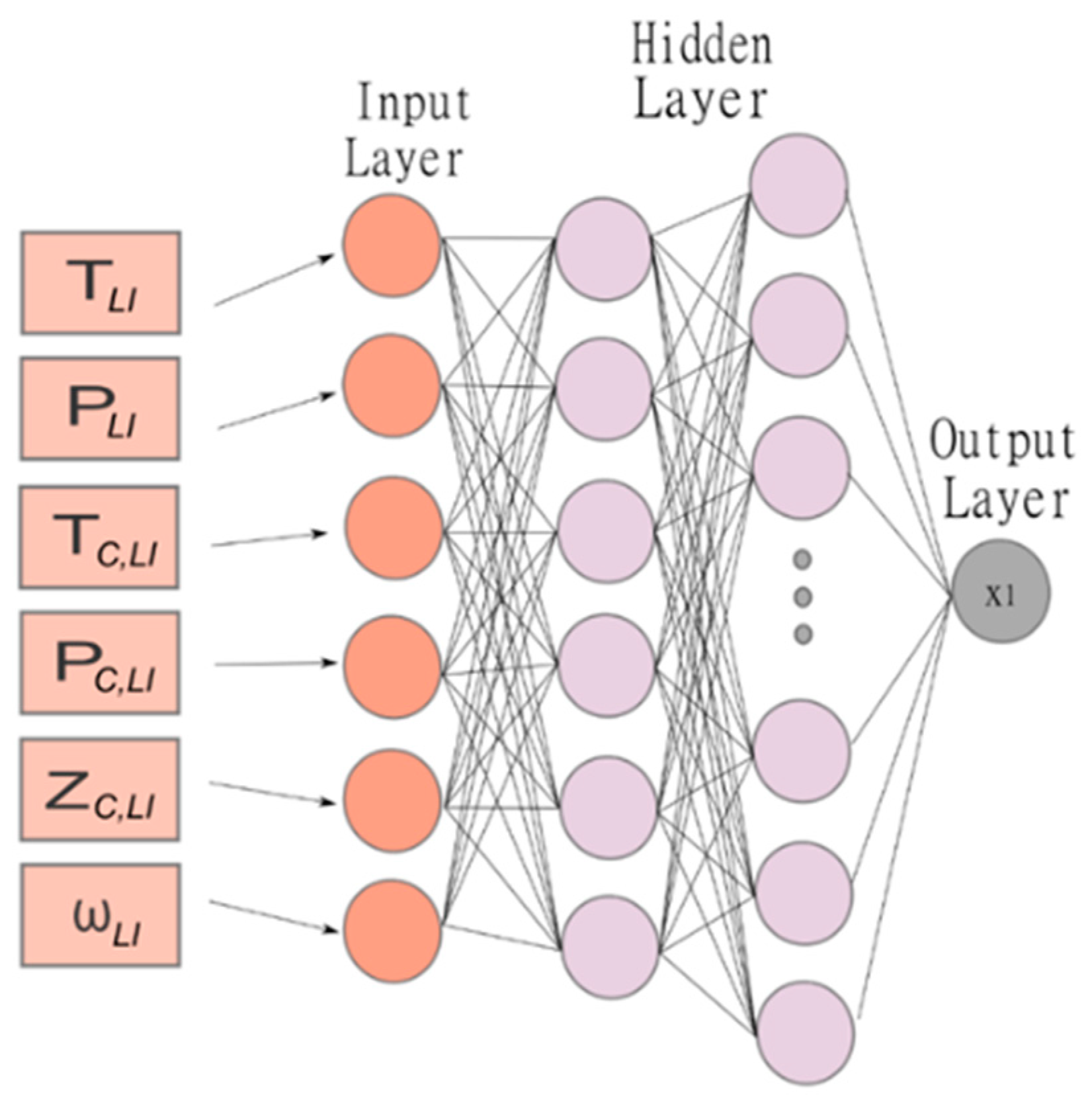
2. Prediction of Solubility by Using a Multilayer Perceptron
3. Results
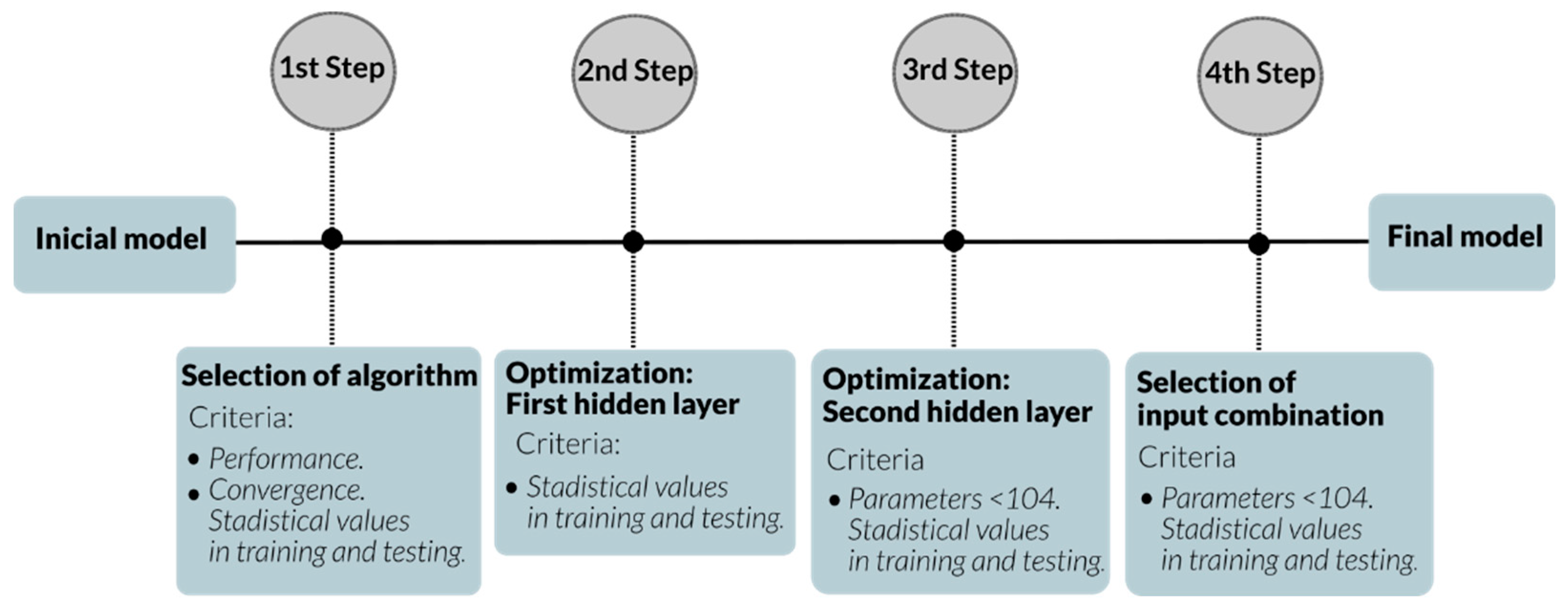
3.1. Selection of Learning Algorithms for Artificial Neural Networks
3.2. Optimization of the First Hidden Layer
3.3. Optimization of the Second Hidden Layer
3.4. Selection of the Input Combination
4. Conclusions
Author Contributions
Funding
Acknowledgments
Conflicts of Interest
References
- Jordaan, S.M.; Romo-Rabago, E.; McLeary, R.; Reidy, L.; Nazari, J.; Herremans, I.M. The role of energy technology innovation in reducing greenhouse gas emissions: A case study of Canada. Renew. Sustain. Energy Rev. 2017, 78, 1397–1409. [Google Scholar] [CrossRef]
- Fernández, Y.F.; López, M.F.; Blanco, B.O. Innovation for sustainability: The impact of R&D spending on CO2 emissions. J. Clean. Prod. 2018, 172, 3459–3467. [Google Scholar]
- Mendelsohn, R.; Neumann, J.E. (Eds.) The Impact of Climate Change on the United States Economy; Cambridge University Press: Cambridge, UK, 2004. [Google Scholar]
- McMichael, A.J.; Woodruff, R.E.; Hales, S. Climate change and human health: Present and future risks. Lancet 2006, 367, 859–869. [Google Scholar] [CrossRef]
- Kjellstrom, T. Impact of climate conditions on occupational health and related economic losses: A new feature of global and urban health in the context of climate change. Asia Pac. J. Public Health 2016, 28 (Suppl. 2), 28S–37S. [Google Scholar] [CrossRef] [PubMed]
- Beller, M.; Steinberg, M. Liquid Fuel Synthesis Using Nuclear Power in a Mobile Energy Depot System (No. BNL-955); Brookhaven National Lab.: Upton, NY, USA, 1965. [Google Scholar]
- Lackner, K.; Ziock, H.J.; Grimes, P. Carbon Dioxide Extraction from Air: Is it an Option? (No. LA-UR-99-583); Los Alamos National Lab.: Los Alamos, NM, USA, 1999. [Google Scholar]
- Keith, D.W.; Holmes, G.; Angelo, D.S.; Heidel, K. A process for capturing CO2 from the atmosphere. Joule 2018, 2, 1573–1594. [Google Scholar] [CrossRef]
- Kanniche, M.; Gros-Bonnivard, R.; Jaud, P.; Valle-Marcos, J.; Amann, J.M.; Bouallou, C. Pre-combustion, post-combustion and oxy-combustion in thermal power plant for CO2 capture. Appl. Therm. Eng. 2010, 30, 53–62. [Google Scholar] [CrossRef]
- Adams, T.A.; Hoseinzade, L.; Madabhushi, P.B.; Okeke, I.J. Comparison of CO2 capture approaches for fossil-based power generation: Review and meta-study. Processes 2017, 5, 44. [Google Scholar] [CrossRef]
- Kohl, A.L.; Nielsen, R. Gas Purification; Elsevier: Amsterdam, The Netherlands, 1997. [Google Scholar]
- Astarita, G.; Savage, D.W.; Longo, J.M. Promotion of CO2 mass transfer in carbonate solutions. Chem. Eng. Sci. 1981, 36, 581–588. [Google Scholar] [CrossRef]
- Tatar, A.; Naseri, S.; Bahadori, M.; Hezave, A.Z.; Kashiwao, T.; Bahadori, A.; Darvish, H. Prediction of carbon dioxide solubility in ionic liquids using MLP and radial basis function (RBF) neural networks. J. Taiwan Inst. Chem. Eng. 2016, 60, 151–164. [Google Scholar] [CrossRef]
- Romeo, L.M.; Minguell, D.; Shirmohammadi, R.; Andrés, J.M. Comparative analysis of the efficiency penalty in power plants of different amine-based solvents for CO2 capture. Ind. Eng. Chem. Res. 2020, 59, 10082–10092. [Google Scholar] [CrossRef]
- Gouedard, C.; Picq, D.; Launay, F.; Carrette, P.L. Amine degradation in CO2 capture. I. A review. Int. J. Greenh. Gas Control. 2012, 10, 244–270. [Google Scholar] [CrossRef]
- Zhang, J.; Nwani, O.; Tan, Y.; Agar, D.W. Carbon dioxide absorption into biphasic amine solvent with solvent loss reduction. Chem. Eng. Res. Des. 2011, 89, 1190–1196. [Google Scholar] [CrossRef]
- Zeng, S.; Zhang, X.; Bai, L.; Zhang, X.; Wang, H.; Wang, J.; Zhang, S. Ionic-liquid-based CO2 capture systems: Structure, interaction and process. Chem. Rev. 2017, 117, 9625–9673. [Google Scholar] [CrossRef] [PubMed]
- Taimoor, A.A.; Al-Shahrani, S.; Muhammad, A. Ionic liquid (1-butyl-3-metylimidazolium methane sulphonate) corrosion and energy analysis for high pressure CO2 absorption process. Processes 2018, 6, 45. [Google Scholar] [CrossRef]
- Leonzio, G.; Zondervan, E. Surface-Response Analysis for the Optimization of a Carbon Dioxide Absorption Process Using [hmim][Tf2N]. Processes 2020, 8, 1063. [Google Scholar] [CrossRef]
- Brennecke, J.F.; Gurkan, B.E. Ionic liquids for CO2 capture and emission reduction. J. Phys. Chem. Lett. 2010, 1, 3459–3464. [Google Scholar] [CrossRef]
- Huang, K.; Peng, H.L. Solubilities of Carbon Dioxide in 1-Ethyl-3-methylimidazolium Thiocyanate, 1-Ethyl-3-methylimidazolium Dicyanamide, and 1-Ethyl-3-methylimidazolium Tricyanomethanide at (298.2 to 373.2) K and (0 to 300.0) kPa. J. Chem. Eng. Data 2017, 62, 4108–4116. [Google Scholar] [CrossRef]
- Kodama, D.; Sato, K.; Watanabe, M.; Sugawara, T.; Makino, T.; Kanakubo, M. Density, Viscosity, and CO2 Solubility in the Ionic Liquid Mixtures of [bmim][PF6] and [bmim][TFSA] at 313.15 K. J. Chem. Eng. Data 2017, 63, 1036–1043. [Google Scholar] [CrossRef]
- Turnaoglu, T.; Minnick, D.L.; Morais, A.R.C.; Baek, D.L.; Fox, R.V.; Scurto, A.M.; Shiflett, M.B. High-pressure vapor− liquid equilibria of 1-alkyl-1-methylpyrrolidinium bis (trifluoromethylsulfonyl) imide ionic liquids and CO2. J. Chem. Eng. Data 2019, 64, 4668–4678. [Google Scholar] [CrossRef]
- Breure, B.; Bottini, S.B.; Witkamp, G.J.; Peters, C.J. Thermodynamic modeling of the phase behavior of binary systems of ionic liquids and carbon dioxide with the group contribution equation of state. J. Phys. Chem. B 2007, 111, 14265–14270. [Google Scholar] [CrossRef]
- Yokozeki, A.; Shiflett, M.B. Gas solubilities in ionic liquids using a generic van der Waals equation of state. J. Supercrit. Fluids 2010, 55, 846–851. [Google Scholar] [CrossRef]
- Kamgar, A.; Rahimpour, M.R. Prediction of CO2 solubility in ionic liquids with QM and UNIQUAC models. J. Mol. Liq. 2016, 222, 195–200. [Google Scholar] [CrossRef]
- Mirzaei, M.; Mokhtarani, B.; Badiei, A.; Sharifi, A. Solubility of carbon dioxide and methane in 1-hexyl-3-methylimidazolium nitrate ionic liquid, experimental and thermodynamic modeling. J. Chem. Thermodyn. 2018, 122, 31–37. [Google Scholar] [CrossRef]
- Venkatraman, V.; Alsberg, B.K. Predicting CO2 capture of ionic liquids using machine learning. J. CO2 Util. 2017, 21, 162–168. [Google Scholar] [CrossRef]
- Mehraein, I.; Riahi, S. The QSPR models to predict the solubility of CO2 in ionic liquids based on least-squares support vector machines and genetic algorithm-multi linear regression. J. Mol. Liq. 2017, 225, 521–530. [Google Scholar] [CrossRef]
- Xia, L.; Wang, J.; Liu, S.; Li, Z.; Pan, H. Prediction of CO2 solubility in ionic liquids based on multi-model fusion method. Processes 2019, 7, 258. [Google Scholar] [CrossRef]
- Xia, L.; Liu, S.; Pan, H. Prediction of the Solubility of CO2 in Imidazolium Ionic Liquids Based on Selective Ensemble Modeling Method. Processes 2020, 8, 1369. [Google Scholar] [CrossRef]
- Song, Z.; Shi, H.; Zhang, X.; Zhou, T. Prediction of CO2 solubility in ionic liquids using machine learning methods. Chem. Eng. Sci. 2020, 223, 115752. [Google Scholar] [CrossRef]
- Nabipour, N.; Mosavi, A.; Baghban, A.; Shamshirband, S.; Felde, I. Extreme learning machine-based model for Solubility estimation of hydrocarbon gases in electrolyte solutions. Processes 2020, 8, 92. [Google Scholar] [CrossRef]
- Yusuf, F.; Olayiwola, T.; Afagwu, C. Application of Artificial Intelligence-based predictive methods in Ionic liquid studies: A review. Fluid Phase Equilibria 2021, 531, 112898. [Google Scholar] [CrossRef]
- Mesbah, M.; Shahsavari, S.; Soroush, E.; Rahaei, N.; Rezakazemi, M. Accurate prediction of miscibility of CO2 and supercritical CO2 in ionic liquids using machine learning. J. CO2 Util. 2018, 25, 99–107. [Google Scholar] [CrossRef]
- Ouaer, H.; Hosseini, A.H.; Nait Amar, M.; El Amine Ben Seghier, M.; Ghriga, M.A.; Nabipour, N.; Shamshirband, S. Rigorous connectionist models to predict carbon dioxide solubility in various ionic liquids. Appl. Sci. 2019, 10, 304. [Google Scholar] [CrossRef]
- Daryayehsalameh, B.; Nabavi, M.; Vaferi, B. Modeling of CO2 capture ability of [Bmim][BF4] ionic liquid using connectionist smart paradigms. Environ. Technol. Innov. 2021, 22, 101484. [Google Scholar] [CrossRef]
- Sedghamiz, M.A.; Rasoolzadeh, A.; Rahimpour, M.R. The ability of artificial neural network in prediction of the acid gases solubility in different ionic liquids. J. CO2 Util. 2015, 9, 39–47. [Google Scholar] [CrossRef]
- Eslamimanesh, A.; Gharagheizi, F.; Mohammadi, A.H.; Richon, D. Artificial neural network modeling of solubility of supercritical carbon dioxide in 24 commonly used ionic liquids. Chem. Eng. Sci. 2011, 66, 3039–3044. [Google Scholar] [CrossRef]
- Rosenblatt, F. The perceptron: A probabilistic model for information storage and organization in the brain. Psychol. Rev. 1958, 65, 386. [Google Scholar] [CrossRef] [PubMed]
- Minsky, M.; Papert, S. Perceptron: An Introduction to Computational Geometry; MIT Press: Cambridge, UK, 1969. [Google Scholar]
- Faúndez, C.A.; Campusano, R.A.; Valderrama, J.O. Misleading results on the use of artificial neural networks for correlating and predicting properties of fluids. A case on the solubility of refrigerant R-32 in ionic liquids. J. Mol. Liq. 2020, 298, 112009. [Google Scholar] [CrossRef]
- Bishop, C. Neural Networks for Pattern Recognition; Oxford University Press: Oxford, UK, 1995. [Google Scholar]
- MATLAB (R2014a). MathWorks. Available online: https://www.mathworks.com/ (accessed on 2 September 2014).
- Fierro, E.N.; Faúndez, C.A.; Muñoz, A.S. Influence of thermodynamically inconsistent data on modeling the solubilities of refrigerants in ionic liquids using an artificial neural network. J. Mol. Liq. 2021, 337, 116417. [Google Scholar] [CrossRef]
- Blanchard, L.A.; Gu, Z.; Brennecke, J.F. High-pressure phase behavior of ionic liquid/CO2 systems. J. Phys. Chem. B 2001, 105, 2437–2444. [Google Scholar] [CrossRef]
- Carvalho, P.J.; Álvarez, V.H.; Machado, J.J.; Pauly, J.; Daridon, J.L.; Marrucho, I.M.; Coutinho, J.A. High pressure phase behavior of carbon dioxide in 1-alkyl-3-methylimidazolium bis (trifluoromethylsulfonyl) imide ionic liquids. J. Supercrit. Fluids 2009, 48, 99–107. [Google Scholar] [CrossRef]
- Carvalho, P.J.; Álvarez, V.H.; Marrucho, I.M.; Aznar, M.; Coutinho, J.A. High pressure phase behavior of carbon dioxide in 1-butyl-3-methylimidazolium bis (trifluoromethylsulfonyl) imide and 1-butyl-3-methylimidazolium dicyanamide ionic liquids. J. Supercrit. Fluids 2009, 50, 105–111. [Google Scholar] [CrossRef]
- Raeissi, S.; Peters, C.J. Carbon dioxide solubility in the homologous 1-alkyl-3-methylimidazolium bis (trifluoromethylsulfonyl) imide family. J. Chem. Eng. Data 2009, 54, 382–386. [Google Scholar] [CrossRef]
- Ren, W.; Sensenich, B.; Scurto, A.M. High-pressure phase equilibria of {carbon dioxide (CO2)+ n-alkyl-imidazolium bis (trifluoromethylsulfonyl) amide} ionic liquids. J. Chem. Thermodyn. 2010, 42, 305–311. [Google Scholar] [CrossRef]
- Shariati, A.; Peters, C.J. High-pressure phase behavior of systems with ionic liquids: Part III. The binary system carbon dioxide+ 1-hexyl-3-methylimidazolium hexafluorophosphate. J. Supercrit. Fluids 2004, 30, 139–144. [Google Scholar] [CrossRef]
- Shiflett, M.B.; Yokozeki, A. Phase behavior of carbon dioxide in ionic liquids:[emim][acetate], [emim][trifluoroacetate], and [emim][acetate] + [emim][trifluoroacetate] mixtures. J. Chem. Eng. Data 2009, 54, 108–114. [Google Scholar] [CrossRef]
- Shin, E.K.; Lee, B.C. High-pressure phase behavior of carbon dioxide with ionic liquids: 1-alkyl-3-methylimidazolium trifluoromethanesulfonate. J. Chem. Eng. Data 2008, 53, 2728–2734. [Google Scholar] [CrossRef]
- Shin, E.K.; Lee, B.C.; Lim, J.S. High-pressure solubilities of carbon dioxide in ionic liquids: 1-alkyl-3-methylimidazolium bis (trifluoromethylsulfonyl) imide. J. Supercrit. Fluids 2008, 45, 282–292. [Google Scholar] [CrossRef]
- Yim, J.H.; Lim, J.S. CO2 solubility measurement in 1-hexyl-3-methylimidazolium ([HMIM]) cation based ionic liquids. Fluid Phase Equilibria 2013, 352, 67–74. [Google Scholar] [CrossRef]
- Safarov, J.; Hamidova, R.; Stephan, M.; Schmotz, N.; Kul, I.; Shahverdiyev, A.; Hassel, E. Carbon dioxide solubility in 1-butyl-3-methylimidazolium-bis (trifluormethylsulfonyl) imide over a wide range of temperatures and pressures. J. Chem. Thermodyn. 2013, 67, 181–189. [Google Scholar] [CrossRef]
- Kim, J.E.; Kim, H.J.; Lim, J.S. Solubility of CO2 in ionic liquids containing cyanide anions:[c2mim][SCN],[c2mim][N (CN) 2],[c2mim][C (CN) 3]. Fluid Phase Equilibria 2014, 367, 151–158. [Google Scholar] [CrossRef]
- Jalili, A.H.; Safavi, M.; Ghotbi, C.; Mehdizadeh, A.; Hosseini-Jenab, M.; Taghikhani, V. Solubility of CO2, H2S, and their mixture in the ionic liquid 1-octyl-3-methylimidazolium bis (trifluoromethyl) sulfonylimide. J. Phys. Chem. B 2012, 116, 2758–2774. [Google Scholar] [CrossRef]
- Afzal, W.; Liu, X.; Prausnitz, J.M. High solubilities of carbon dioxide in tetraalkyl phosphonium-based ionic liquids and the effect of diluents on viscosity and solubility. J. Chem. Eng. Data 2014, 59, 954–960. [Google Scholar] [CrossRef]
- Hwang, S.; Park, Y.; Park, K. Phase equilibria of the 1-hexyl-2, 3-dimethylimidazolium bis (trifluoromethylsulfonyl) imide and carbon dioxide binary system and 1-octyl-2, 3-dimethylimidazolium bis (trifluoromethylsulfonyl) imide and carbon dioxide binary system. J. Chem. Eng. Data 2012, 57, 2160–2164. [Google Scholar] [CrossRef]
- Revelli, A.L.; Mutelet, F.; Jaubert, J.N. High carbon dioxide solubilities in imidazolium-based ionic liquids and in poly (ethylene glycol) dimethyl ether. J. Phys. Chem. B 2010, 114, 12908–12913. [Google Scholar] [CrossRef] [PubMed]
- Yim, J.H.; Song, H.N.; Yoo, K.P.; Lim, J.S. Measurement of CO2 solubility in ionic liquids:[BMP][Tf2N] and [BMP][MeSO4] by measuring bubble-point pressure. J. Chem. Eng. Data 2011, 56, 1197–1203. [Google Scholar] [CrossRef]
- Yim, J.H.; Ha, S.J.; Lim, J.S. Measurement and Correlation of CO2 Solubility in 1-Ethyl-3-methylimidazolium ([EMIM]) Cation-Based Ionic Liquids:[EMIM][Ac],[EMIM][Cl], and [EMIM][MeSO4]. J. Chem. Eng. Data 2018, 63, 508–518. [Google Scholar] [CrossRef]
- Ramdin, M.; Vlugt, T.J.; de Loos, T.W. Solubility of CO2 in the ionic liquids [TBMN][MeSO4] and [TBMP][MeSO4]. J. Chem. Eng. Data 2012, 57, 2275–2280. [Google Scholar] [CrossRef]
- Song, H.N.; Lee, B.C.; Lim, J.S. Measurement of CO2 solubility in ionic liquids: [BMP][TfO] and [P14, 6, 6, 6][Tf2N] by measuring bubble-point pressure. J. Chem. Eng. Data 2010, 55, 891–896. [Google Scholar] [CrossRef]
- Jang, S.; Cho, D.W.; Im, T.; Kim, H. High-pressure phase behavior of CO2+ 1-butyl-3-methylimidazolium chloride system. Fluid Phase Equilibria 2010, 299, 216–221. [Google Scholar] [CrossRef]
- Tagiuri, A.; Sumon, K.Z.; Henni, A. Solubility of carbon dioxide in three [Tf2N] ionic liquids. Fluid Phase Equilibria 2014, 380, 39–47. [Google Scholar] [CrossRef]
- Watanabe, M.; Kodama, D.; Makino, T.; Kanakubo, M. CO2 absorption properties of imidazolium based ionic liquids using a magnetic suspension balance. Fluid Phase Equilibria 2016, 420, 44–49. [Google Scholar] [CrossRef]
- Zoubeik, M.; Mohamedali, M.; Henni, A. Experimental solubility and thermodynamic modeling of CO2 in four new imidazolium and pyridinium-based ionic liquids. Fluid Phase Equilibria 2016, 419, 67–74. [Google Scholar] [CrossRef]
- Safavi, M.; Ghotbi, C.; Taghikhani, V.; Jalili, A.H.; Mehdizadeh, A. Study of the solubility of CO2, H2S and their mixture in the ionic liquid 1-octyl-3-methylimidazolium hexafluorophosphate: Experimental and modelling. J. Chem. Thermodyn. 2013, 65, 220–232. [Google Scholar] [CrossRef]
- Ebrahiminejadhasanabadi, M.; Nelson, W.M.; Naidoo, P.; Mohammadi, A.H.; Ramjugernath, D. Experimental measurement of carbon dioxide solubility in 1-methylpyrrolidin-2-one (NMP)+ 1-butyl-3-methyl-1H-imidazol-3-ium tetrafluoroborate ([bmim][BF4]) mixtures using a new static-synthetic cell. Fluid Phase Equilibria 2018, 477, 62–77. [Google Scholar] [CrossRef]
- Baghban, A.; Ahmadi, M.A.; Shahraki, B.H. Prediction carbon dioxide solubility in presence of various ionic liquids using computational intelligence approaches. J. Supercrit. Fluids 2015, 98, 50–64. [Google Scholar] [CrossRef]
- Faúndez, C.A.; Fierro, E.N.; Valderrama, J.O. Solubility of hydrogen sulfide in ionic liquids for gas removal processes using artificial neural networks. J. Environ. Chem. Eng. 2016, 4, 211–218. [Google Scholar] [CrossRef]
- Valderrama, J.O.; Forero, L.A.; Rojas, R.E. Extension of a group contribution method to estimate the critical properties of ionic liquids of high molecular mass. Ind. Eng. Chem. Res. 2015, 54, 3480–3487. [Google Scholar] [CrossRef]


| Author | Data Point Studied | Data Point Predicted | System | R2 | Architecture | Input | Np* |
|---|---|---|---|---|---|---|---|
| Ouaer et al., 2019 [36] | 744 | 149 | 13 | 0.9971 | (6,11,11,9,1) | T, P, Mw, Tc, Pc, w | 327 |
| Sedghamiz et al., 2015 [38] | 2930 | 440 | 39 | 0.9947 | (5,23,1) | T, P, Tc, Pc, w | 162 |
| Tatar et al., 2016 [13] | 728 | 146 | 14 | 0.998272 | (5,23,1) | T, P, Tc, Pc, w | 162 |
| Mesbah et al., 2018 [35] | 1386 | 208 | 20 | 0.9987 | (5,15,10,1) | Mw, Tc, Pc, T, P | 261 |
| Eslamimaneash et al., 2011 [39] | 1128 | 112 | 24 | 0.0995 | (5,19,1) | T, P, Tc, Pc, w | 134 |
| Song et al., 2020 [32] | 10,116 | 2023 | 124 | 0.0202 | (53,7,1) | 51 group numbers, T and P | 386 |
| Daryayehsalameh et al., 2021 [37] | 548 | 110 | 17 | 0.98684 | (2,6,1) | T and P | 25 |
| Systems | n | T(K) | P (MPa) | x1 | Ref. | ||||||
|---|---|---|---|---|---|---|---|---|---|---|---|
| (Bmim)(PF6) | 7 | 313.00 | 1.5170 | - | 9.5670 | 0.2310 | - | 0.7290 | [46] | ||
| 7 | 323.00 | 1.7380 | - | 9.2460 | 0.2360 | - | 0.6750 | ||||
| 7 | 333.00 | 1.5790 | - | 9.3010 | 0.2280 | - | 0.6670 | ||||
| (Bmim)(NO3) | 7 | 313.00 | 1.5470 | - | 9.2000 | 0.1960 | - | 0.5130 | |||
| 7 | 323.00 | 1.7120 | - | 9.2620 | 0.1690 | - | 0.5300 | ||||
| 7 | 333.00 | 1.8370 | - | 9.3170 | 0.1830 | - | 0.5220 | ||||
| (Omim)(BF4) | 7 | 313.00 | 1.7260 | - | 9.2900 | 0.1970 | - | 0.7080 | |||
| 7 | 323.00 | 1.5610 | - | 9.2280 | 0.1910 | - | 0.6710 | ||||
| 7 | 333.00 | 1.5610 | - | 9.3730 | 0.1600 | - | 0.6510 | ||||
| (Emim)(Tf2N) | 9 | 292.16 | - | 293.65 | 0.6200 | - | 16.0760 | 0.2210 | - | 0.7500 | [47] |
| 9 | 297.70 | - | 298.55 | 0.7250 | - | 19.0480 | 0.2210 | - | 0.7500 | ||
| 9 | 303.25 | - | 303.54 | 0.8370 | - | 22.1300 | 0.2210 | - | 0.7500 | ||
| 9 | 313.19 | - | 313.59 | 1.0830 | - | 28.1870 | 0.2210 | - | 0.7500 | ||
| 9 | 323.09 | - | 323.27 | 1.3450 | - | 33.7870 | 0.2210 | - | 0.7500 | ||
| 9 | 332.88 | - | 333.23 | 1.6450 | - | 38.8980 | 0.2210 | - | 0.7500 | ||
| 9 | 343.08 | - | 343.30 | 1.9570 | - | 43.5650 | 0.2210 | - | 0.7500 | ||
| 9 | 353.02 | - | 353.22 | 2.2760 | - | 47.8500 | 0.2210 | - | 0.7500 | ||
| 8 | 363.17 | - | 363.55 | 2.6800 | - | 30.8580 | 0.2210 | - | 0.7000 | ||
| (Pmim)(Tf2N) | 9 | 293.30 | - | 293.76 | 0.6180 | - | 27.4600 | 0.2120 | - | 0.8020 | |
| 9 | 298.37 | - | 298.77 | 0.7200 | - | 30.0980 | 0.2120 | - | 0.8020 | ||
| 9 | 303.33 | - | 303.61 | 0.7990 | - | 32.8810 | 0.2120 | - | 0.8020 | ||
| 9 | 312.85 | - | 313.57 | 1.0440 | - | 38.2990 | 0.2120 | - | 0.8020 | ||
| 9 | 322.52 | - | 323.35 | 1.2520 | - | 43.2250 | 0.2120 | - | 0.8020 | ||
| 9 | 332.54 | - | 333.56 | 1.5250 | - | 47.9600 | 0.2120 | - | 0.8020 | ||
| 9 | 342.47 | - | 343.37 | 1.7800 | - | 52.4310 | 0.2120 | - | 0.8020 | ||
| 9 | 352.65 | - | 353.49 | 2.1240 | - | 56.1460 | 0.2120 | - | 0.8020 | ||
| 9 | 362.95 | - | 363.29 | 2.3700 | - | 59.8050 | 0.2120 | - | 0.8020 | ||
| (Bmim)(Tf 2N) | 9 | 292.65 | - | 293.53 | 0.6290 | - | 33.2630 | 0.2310 | - | 0.8010 | [48] |
| 9 | 303.05 | - | 303.31 | 0.7860 | - | 39.3730 | 0.2310 | - | 0.8010 | ||
| 9 | 313.10 | - | 313.32 | 0.2310 | - | 44.7400 | 0.2310 | - | 0.8010 | ||
| 9 | 323.09 | - | 323.30 | 1.3030 | - | 49.9900 | 0.2310 | - | 0.8010 | ||
| 8 | 333.10 | - | 333.28 | 1.5740 | - | 33.6930 | 0.2310 | - | 0.7710 | ||
| 8 | 342.87 | - | 343.25 | 1.8740 | - | 38.0810 | 0.2310 | - | 0.7710 | ||
| 8 | 353.09 | - | 353.22 | 2.1790 | - | 42.0300 | 0.2310 | - | 0.7710 | ||
| 8 | 362.99 | - | 363.18 | 2.4850 | - | 46.0100 | 0.2310 | - | 0.7710 | ||
| (Bmim)(DCA) | 5 | 293.36 | - | 293.50 | 1.0180 | - | 32.6060 | 0.2000 | - | 0.6010 | |
| 5 | 302.91 | - | 303.45 | 1.3600 | - | 39.8660 | 0.2000 | - | 0.6010 | ||
| 5 | 313.03 | - | 313.36 | 1.7710 | - | 46.7490 | 0.2000 | - | 0.6010 | ||
| 5 | 322.93 | - | 323.47 | 2.2600 | - | 53.1740 | 0.2000 | - | 0.6010 | ||
| 5 | 332.72 | - | 333.28 | 2.6440 | - | 59.0070 | 0.2000 | - | 0.6010 | ||
| 5 | 343.01 | - | 343.34 | 3.1080 | - | 64.2170 | 0.2000 | - | 0.6010 | ||
| 5 | 353.09 | - | 353.01 | 3.7450 | - | 69.0020 | 0.2000 | - | 0.6010 | ||
| 5 | 363.11 | - | 363.25 | 4.3280 | - | 73.6400 | 0.2000 | - | 0.6010 | ||
| (Bmim)(Tf2N) | 6 | 371.43 | - | 371.59 | 2.2020 | - | 13.9590 | 0.1886 | - | 0.5852 | [49] |
| 4 | 380.99 | - | 381.22 | 2.4330 | - | 11.6250 | 0.1886 | - | 0.5257 | ||
| 5 | 390.86 | - | 390.95 | 2.6680 | - | 12.8740 | 0.1886 | - | 0.5257 | ||
| 4 | 400.59 | - | 400.64 | 2.9120 | - | 14.0990 | 0.1886 | - | 0.5257 | ||
| 4 | 410.37 | - | 410.52 | 3.1580 | - | 13.4730 | 0.1886 | - | 0.4866 | ||
| 3 | 420.12 | - | 420.21 | 3.3980 | - | 8.9330 | 0.1886 | - | 0.3818 | ||
| 3 | 429.86 | - | 429.89 | 3.6480 | - | 9.5480 | 0.1886 | - | 0.3818 | ||
| 3 | 439.60 | - | 439.65 | 3.8880 | - | 10.1980 | 0.1886 | - | 0.3818 | ||
| 3 | 449.36 | - | 449.41 | 4.1330 | - | 10.8330 | 0.1886 | - | 0.3818 | ||
| (EMIm)(Tf2N) | 7 | 298.15 | 1.2350 | - | 14.7940 | 0.2800 | - | 0.7820 | [50] | ||
| (HMIm)(Tf2N) | 8 | 298.15 | 2.0150 | - | 14.8040 | 0.3960 | - | 0.8230 | |||
| 9 | 323.15 | 3.7160 | - | 12.9590 | 0.4870 | - | 0.7790 | ||||
| 7 | 343.15 | 2.7540 | - | 24.7080 | 0.2390 | - | 0.7710 | ||||
| (Hmim)(PF6) | 3 | 358.45 | - | 358.65 | 2.9200 | - | 8.4100 | 0.1980 | - | 0.4100 | [51] |
| 6 | 347.65 | - | 348.63 | 2.5700 | - | 76.9000 | 0.1980 | - | 0.7110 | ||
| 9 | 337.82 | - | 338.47 | 2.2600 | - | 92.5000 | 0.1980 | - | 0.7270 | ||
| 9 | 327.74 | - | 328.58 | 1.9400 | - | 87.5800 | 0.1980 | - | 0.7270 | ||
| 9 | 318.03 | - | 318.55 | 1.6500 | - | 82.8000 | 0.1980 | - | 0.7270 | ||
| 3 | 303.34 | - | 303.48 | 1.2700 | - | 3.3700 | 0.1980 | - | 0.4100 | ||
| 3 | 308.35 | - | 308.48 | 1.4000 | - | 3.8000 | 0.1980 | - | 0.4100 | ||
| 2 | 298.31 | - | 298.45 | 1.1500 | - | 3.0500 | 0.1980 | - | 0.4100 | ||
| (Emim)(Ac) | 9 | 298.10 | 0.0100 | - | 1.9998 | 0.1890 | - | 0.4280 | [52] | ||
| 8 | 323.10 | 0.0499 | - | 1.9996 | 0.2030 | - | 0.3900 | ||||
| 8 | 348.10 | - | 348.20 | 0.0501 | - | 1.9996 | 0.1570 | - | 0.3210 | ||
| (Emim)(TfO) | 11 | 303.85 | 0.8000 | - | 14.9000 | 0.1794 | - | 0.6268 | [53] | ||
| 11 | 314.05 | 1.0000 | - | 21.0000 | 0.1794 | - | 0.6268 | ||||
| 11 | 324.15 | 1.1500 | - | 27.0000 | 0.1794 | - | 0.6268 | ||||
| 11 | 334.35 | 1.3000 | - | 32.6000 | 0.1794 | - | 0.6268 | ||||
| 11 | 344.55 | 1.5500 | - | 37.8000 | 0.1794 | - | 0.6268 | ||||
| (Bmim)(TfO) | 13 | 303.85 | 0.8500 | - | 16.0000 | 0.2182 | - | 0.6720 | |||
| 13 | 314.05 | 1.0200 | - | 22.0000 | 0.2182 | - | 0.6720 | ||||
| 13 | 324.15 | 1.1500 | - | 27.4000 | 0.2182 | - | 0.6720 | ||||
| 13 | 334.35 | 1.3500 | - | 32.4000 | 0.2182 | - | 0.6720 | ||||
| 13 | 344.55 | 1.9000 | - | 37.5000 | 0.2182 | - | 0.6720 | ||||
| (Omim)(TfO) | 13 | 303.85 | 0.6800 | - | 18.0000 | 0.2166 | - | 0.7414 | |||
| 13 | 314.05 | 0.8000 | - | 22.0000 | 0.2166 | - | 0.7414 | ||||
| 13 | 324.15 | 1.0800 | - | 25.8000 | 0.2166 | - | 0.7414 | ||||
| 13 | 334.35 | 1.3500 | - | 29.8000 | 0.2166 | - | 0.7414 | ||||
| 13 | 344.55 | 1.6500 | - | 34.0000 | 0.2166 | - | 0.7414 | ||||
| (Emim)(Tf2N) | 12 | 344.40 | 3.0600 | - | 43.2000 | 0.2330 | - | 0.7610 | [54] | ||
| 12 | 334.20 | 2.6600 | - | 36.5000 | 0.2330 | - | 0.7610 | ||||
| 12 | 324.00 | 2.2000 | - | 30.9000 | 0.2330 | - | 0.7610 | ||||
| 12 | 313.90 | 1.8300 | - | 25.3000 | 0.2330 | - | 0.7610 | ||||
| 12 | 303.70 | 1.5300 | - | 18.8000 | 0.2330 | - | 0.7610 | ||||
| 22 | 292.90 | - | 295.40 | 1.2200 | - | 17.0600 | 0.2330 | - | 0.8032 | ||
| 13 | 303.70 | - | 303.90 | 1.8400 | - | 22.4500 | 0.3970 | - | 0.8032 | ||
| 13 | 313.90 | 2.1400 | - | 28.0700 | 0.3970 | - | 0.8032 | ||||
| 13 | 324.00 | 2.4500 | - | 33.3500 | 0.3970 | - | 0.8032 | ||||
| 13 | 334.20 | 2.9200 | - | 38.2500 | 0.3970 | - | 0.8032 | ||||
| 13 | 344.40 | 3.6400 | - | 42.8000 | 0.3970 | - | 0.8032 | ||||
| (Hmim)(Tf2N) | 18 | 303.70 | 1.4000 | - | 20.4000 | 0.3221 | - | 0.8333 | |||
| 18 | 313.90 | 1.7500 | - | 25.3000 | 0.3221 | - | 0.8333 | ||||
| 18 | 324.00 | 2.1000 | - | 30.2000 | 0.3221 | - | 0.8333 | ||||
| 18 | 334.20 | 2.5200 | - | 34.5000 | 0.3221 | - | 0.8333 | ||||
| 18 | 344.40 | 2.9600 | - | 39.0000 | 0.3221 | - | 0.8333 | ||||
| (Omim)(Tf2N) | 7 | 297.40 | - | 298.80 | 1.2300 | - | 14.8000 | 0.3762 | - | 0.8456 | |
| 9 | 299.80 | - | 301.30 | 0.6800 | - | 6.7000 | 0.3019 | - | 0.8120 | ||
| 16 | 303.70 | 0.7200 | - | 17.0000 | 0.3019 | - | 0.8456 | ||||
| 16 | 313.90 | 0.8200 | - | 22.0000 | 0.3019 | - | 0.8456 | ||||
| 16 | 324.00 | 0.9600 | - | 26.0000 | 0.3019 | - | 0.8456 | ||||
| 16 | 334.20 | 1.2800 | - | 30.7000 | 0.3019 | - | 0.8456 | ||||
| 16 | 344.40 | 1.6000 | - | 34.8000 | 0.3019 | - | 0.8456 | ||||
| (HMIM)(Tf2N) | 8 | 303.15 | 0.4200 | - | 11.4900 | 0.1650 | - | 0.8240 | [55] | ||
| 8 | 313.15 | 0.5800 | - | 18.2700 | 0.1650 | - | 0.8240 | ||||
| 8 | 323.15 | 0.6700 | - | 22.6300 | 0.1650 | - | 0.8240 | ||||
| 8 | 333.15 | 0.8000 | - | 27.8000 | 0.1650 | - | 0.8240 | ||||
| 8 | 343.15 | 0.9600 | - | 31.2700 | 0.1650 | - | 0.8240 | ||||
| 8 | 353.15 | 1.0900 | - | 36.6300 | 0.1650 | - | 0.8240 | ||||
| 8 | 363.15 | 1.2400 | - | 42.8900 | 0.1650 | - | 0.8240 | ||||
| 8 | 373.15 | 1.3800 | - | 45.2800 | 0.1650 | - | 0.8240 | ||||
| (HMIM)(TfO) | 8 | 303.15 | 1.4200 | - | 67.9700 | 0.2670 | - | 0.8160 | |||
| 8 | 313.15 | 1.7600 | - | 73.9500 | 0.2670 | - | 0.8160 | ||||
| 8 | 323.15 | 2.2500 | - | 78.0000 | 0.2670 | - | 0.8160 | ||||
| 8 | 333.15 | 2.6500 | - | 81.7300 | 0.2670 | - | 0.8160 | ||||
| 8 | 343.15 | 3.1000 | - | 86.1200 | 0.2670 | - | 0.8160 | ||||
| 8 | 353.15 | 3.6600 | - | 89.8900 | 0.2670 | - | 0.8160 | ||||
| 8 | 363.15 | 4.0200 | - | 95.3100 | 0.2670 | - | 0.8160 | ||||
| 8 | 373.15 | 4.4600 | - | 100.1200 | 0.2670 | - | 0.8160 | ||||
| (HMIM)(BF4) | 6 | 303.15 | 1.2000 | - | 8.7700 | 0.2120 | - | 0.6220 | |||
| 6 | 313.15 | 1.5300 | - | 16.2000 | 0.2120 | - | 0.6220 | ||||
| 6 | 323.15 | 1.9300 | - | 22.2800 | 0.2120 | - | 0.6220 | ||||
| 6 | 333.15 | 2.3200 | - | 27.1600 | 0.2120 | - | 0.6220 | ||||
| 6 | 343.15 | 2.6800 | - | 32.2600 | 0.2120 | - | 0.6220 | ||||
| 6 | 353.15 | 3.1400 | - | 36.0500 | 0.2120 | - | 0.6220 | ||||
| 6 | 363.15 | 3.4700 | - | 39.3500 | 0.2120 | - | 0.6220 | ||||
| 6 | 373.15 | 3.7600 | - | 41.6900 | 0.2120 | - | 0.6220 | ||||
| (Hmim)(PF6) | 6 | 303.15 | 0.3000 | - | 26.5400 | 0.2160 | - | 0.6910 | |||
| 6 | 313.15 | 0.5300 | - | 34.0100 | 0.2160 | - | 0.6910 | ||||
| 6 | 323.15 | 0.8600 | - | 39.5200 | 0.2160 | - | 0.6910 | ||||
| 6 | 333.15 | 1.2200 | - | 43.9100 | 0.2160 | - | 0.6910 | ||||
| 6 | 343.15 | 1.5300 | - | 47.4700 | 0.2160 | - | 0.6910 | ||||
| 6 | 353.15 | 1.7200 | - | 50.2500 | 0.2160 | - | 0.6910 | ||||
| 6 | 363.15 | 1.9400 | - | 53.2800 | 0.2160 | - | 0.6910 | ||||
| 6 | 373.15 | 2.1900 | - | 55.6300 | 0.2160 | - | 0.6910 | ||||
| (HMIM)(NTf2) | 3 | 273.15 | 0.3990 | - | 2.4790 | 0.1852 | - | 0.6425 | [56] | ||
| 4 | 293.15 | 0.4270 | - | 4.1550 | 0.6555 | - | 0.1401 | ||||
| 4 | 313.15 | 0.4460 | - | 4.3510 | 0.1095 | - | 0.5665 | ||||
| 3 | 333.15 | 1.2340 | - | 4.4710 | 0.2153 | - | 0.4921 | ||||
| 3 | 353.15 | 1.2610 | - | 4.5470 | 0.2454 | - | 0.4393 | ||||
| 3 | 373.15 | 1.2810 | - | 4.6030 | 0.1632 | - | 0.3966 | ||||
| 3 | 393.15 | 1.2980 | - | 4.6430 | 0.1455 | - | 0.3683 | ||||
| 3 | 413.15 | 1.3110 | - | 4.6740 | 0.1342 | - | 0.3481 | ||||
| (Emim)(SCN) | 9 | 303.15 | 1.3000 | - | 74.4100 | 0.1690 | - | 0.4740 | [57] | ||
| 9 | 313.15 | 1.6800 | - | 79.5300 | 0.1690 | - | 0.4740 | ||||
| 9 | 323.15 | 1.9800 | - | 83.9000 | 0.1690 | - | 0.4740 | ||||
| 9 | 333.15 | 2.4000 | - | 88.0000 | 0.1690 | - | 0.4740 | ||||
| 9 | 343.15 | 2.8500 | - | 90.4600 | 0.1690 | - | 0.4740 | ||||
| 9 | 353.15 | 3.3700 | - | 93.0000 | 0.1690 | - | 0.4740 | ||||
| 9 | 363.15 | 3.8900 | - | 94.4000 | 0.1690 | - | 0.4740 | ||||
| 9 | 373.15 | 4.4700 | - | 95.3400 | 0.1690 | - | 0.4740 | ||||
| (Emim)(N(CN)2) | 10 | 303.15 | 0.8800 | - | 61.0800 | 0.1710 | - | 0.5850 | |||
| 10 | 313.15 | 1.0600 | - | 67.4800 | 0.1710 | - | 0.5850 | ||||
| 10 | 323.15 | 1.3400 | - | 73.2200 | 0.1710 | - | 0.5850 | ||||
| 10 | 333.15 | 1.5700 | - | 78.7800 | 0.1710 | - | 0.5850 | ||||
| 10 | 343.15 | 1.9000 | - | 83.6700 | 0.1710 | - | 0.5850 | ||||
| 10 | 353.15 | 2.2800 | - | 88.1500 | 0.1710 | - | 0.5850 | ||||
| 10 | 363.15 | 2.5800 | - | 92.2900 | 0.1710 | - | 0.5850 | ||||
| 10 | 373.15 | 2.8900 | - | 96.2000 | 0.1710 | - | 0.5850 | ||||
| (Emim)(C(CN)3) | 10 | 303.15 | 0.5900 | - | 46.9600 | 0.1700 | - | 0.7030 | |||
| 10 | 313.15 | 0.9100 | - | 54.2400 | 0.1700 | - | 0.7030 | ||||
| 10 | 323.15 | 1.2100 | - | 60.3100 | 0.1700 | - | 0.7030 | ||||
| 10 | 333.15 | 1.4100 | - | 66.7700 | 0.1700 | - | 0.7030 | ||||
| 10 | 343.15 | 1.6500 | - | 72.8500 | 0.1700 | - | 0.7030 | ||||
| 10 | 353.15 | 1.9500 | - | 78.4400 | 0.1700 | - | 0.7030 | ||||
| 10 | 363.15 | 2.2100 | - | 83.4900 | 0.1700 | - | 0.7030 | ||||
| 10 | 373.15 | 2.4300 | - | 88.2900 | 0.1700 | - | 0.7030 | ||||
| (Omim)(Tf2N) | 5 | 303.15 | 0.4147 | - | 1.5893 | 0.1380 | - | 0.4012 | [58] | ||
| 5 | 313.15 | 0.4405 | - | 1.6922 | 0.1297 | - | 0.3846 | ||||
| 5 | 323.15 | 0.4649 | - | 1.7909 | 0.1227 | - | 0.3685 | ||||
| 5 | 333.15 | 0.4880 | - | 1.8856 | 0.1170 | - | 0.3562 | ||||
| 5 | 343.15 | 0.5101 | - | 1.9760 | 0.1123 | - | 0.3445 | ||||
| 5 | 353.15 | 0.5314 | - | 2.0628 | 0.1087 | - | 0.3433 | ||||
| (P(14)666)(DCA) | 5 | 298.00 | - | 299.00 | 0.7920 | - | 2.6540 | 0.2250 | - | 0.5270 | [59] |
| 5 | 303.00 | - | 304.00 | 0.8240 | - | 2.7740 | 0.2180 | - | 0.5170 | ||
| 5 | 313.00 | 0.8860 | - | 3.0080 | 0.2020 | - | 0.4980 | ||||
| 5 | 322.00 | - | 323.00 | 0.9370 | - | 3.2290 | 0.1920 | - | 0.4810 | ||
| (HMMIM)(Tf2N) | 5 | 298.20 | 1.1050 | - | 6.3430 | 0.2106 | - | 0.8014 | [60] | ||
| 7 | 303.20 | 1.2040 | - | 6.6400 | 0.1642 | - | 0.8014 | ||||
| 7 | 308.20 | 1.3190 | - | 6.8790 | 0.1642 | - | 0.8014 | ||||
| 7 | 313.20 | 1.4110 | - | 7.0720 | 0.1642 | - | 0.8014 | ||||
| 7 | 318.20 | 1.5770 | - | 7.1960 | 0.1642 | - | 0.8014 | ||||
| 3 | 323.20 | 1.9100 | - | 5.4970 | 0.2106 | - | 0.5991 | ||||
| (BMIM)(BF4) | 6 | 293.15 | - | 293.75 | 1.0500 | - | 7.3000 | 0.1410 | - | 0.6100 | [61] |
| 6 | 303.15 | - | 303.85 | 1.2000 | - | 8.1000 | 0.1410 | - | 0.6100 | ||
| 6 | 313.25 | - | 314.05 | 1.3900 | - | 10.5000 | 0.1410 | - | 0.6100 | ||
| |6 | 322.65 | - | 324.15 | 1.5800 | - | 14.1000 | 0.1410 | - | 0.6100 | ||
| 6 | 333.05 | - | 333.95 | 1.7800 | - | 16.2000 | 0.1410 | - | 0.6100 | ||
| 6 | 342.75 | - | 343.75 | 2.0300 | - | 18.8500 | 0.1410 | - | 0.6100 | ||
| 6 | 352.05 | - | 354.25 | 2.4100 | - | 22.3300 | 0.1410 | - | 0.6100 | ||
| 6 | 362.85 | - | 363.15 | 2.7200 | - | 24.6000 | 0.1410 | - | 0.6100 | ||
| 5 | 373.15 | - | 373.45 | 3.0300 | - | 19.8000 | 0.1410 | - | 0.5000 | ||
| 5 | 382.95 | - | 383.15 | 3.8000 | - | 23.5000 | 0.1410 | - | 0.5000 | ||
| (BMIM)(SCN) | 4 | 292.35 | - | 293.65 | 1.0500 | - | 4.3500 | 0.1260 | - | 0.2960 | |
| 5 | 302.55 | - | 303.35 | 1.3100 | - | 5.5000 | 0.1260 | - | 0.3370 | ||
| 6 | 312.75 | - | 313.65 | 1.6000 | - | 9.9000 | 0.1260 | - | 0.4300 | ||
| 6 | 322.75 | - | 324.65 | 1.9200 | - | 12.8000 | 0.1260 | - | 0.4300 | ||
| 6 | 332.95 | - | 333.65 | 2.3100 | - | 16.7000 | 0.1260 | - | 0.4300 | ||
| 6 | 342.55 | - | 344.15 | 2.6800 | - | 20.5000 | 0.1260 | - | 0.4300 | ||
| 6 | 352.85 | - | 353.55 | 3.0500 | - | 24.2000 | 0.1260 | - | 0.4300 | ||
| 6 | 361.45 | - | 363.35 | 3.5500 | - | 27.5000 | 0.1260 | - | 0.4300 | ||
| 6 | 372.55 | - | 373.35 | 4.0800 | - | 31.5000 | 0.1260 | - | 0.4300 | ||
| 5 | 381.95 | - | 384.15 | 4.4600 | - | 12.1100 | 0.1260 | - | 0.3370 | ||
| (BMP)(Tf2N) | 9 | 303.15 | 0.6800 | - | 35.1600 | 0.2276 | - | 0.8029 | [62] | ||
| 9 | 313.15 | 0.9900 | - | 39.3400 | 0.2276 | - | 0.8029 | ||||
| 9 | 323.15 | 1.2300 | - | 44.5400 | 0.2276 | - | 0.8029 | ||||
| 9 | 333.15 | 1.4000 | - | 48.4000 | 0.2276 | - | 0.8029 | ||||
| 9 | 343.15 | 1.5600 | - | 52.7500 | 0.2276 | - | 0.8029 | ||||
| 9 | 353.15 | 1.8200 | - | 56.2300 | 0.2276 | - | 0.8029 | ||||
| 9 | 363.15 | 2.0400 | - | 59.4400 | 0.2276 | - | 0.8029 | ||||
| 9 | 373.15 | 2.2600 | - | 62.7700 | 0.2276 | - | 0.8029 | ||||
| (EMIM)(Ac) | 8 | 303.15 | 0.4500 | - | 5.8700 | 0.2950 | - | 0.5750 | [63] | ||
| 8 | 313.15 | 0.5700 | - | 7.6300 | 0.2950 | - | 0.5750 | ||||
| 8 | 323.15 | 0.7400 | - | 9.4600 | 0.2950 | - | 0.5750 | ||||
| 8 | 333.15 | 0.9300 | - | 11.8200 | 0.2950 | - | 0.5750 | ||||
| 8 | 343.15 | 1.1800 | - | 14.6100 | 0.2950 | - | 0.5750 | ||||
| 8 | 353.15 | 1.4400 | - | 17.8500 | 0.2950 | - | 0.5750 | ||||
| 8 | 363.15 | 1.7000 | - | 20.9600 | 0.2950 | - | 0.5750 | ||||
| 8 | 373.15 | 2.0100 | - | 24.6400 | 0.2950 | - | 0.5750 | ||||
| (TBMA)(MeSO4) | 3 | 338.40 | - | 338.41 | 2.4500 | - | 8.0290 | 0.1530 | - | 0.3680 | [64] |
| 3 | 343.29 | - | 343.44 | 2.6100 | - | 8.5740 | 0.1530 | - | 0.3680 | ||
| 3 | 348.36 | - | 348.48 | 2.7600 | - | 9.1740 | 0.1530 | - | 0.3680 | ||
| 3 | 353.35 | - | 353.53 | 2.9300 | - | 9.7410 | 0.1530 | - | 0.3680 | ||
| 3 | 358.43 | - | 358.56 | 3.0800 | - | 10.3370 | 0.1530 | - | 0.3680 | ||
| 3 | 363.41 | - | 363.50 | 3.1960 | - | 10.9530 | 0.1530 | - | 0.3680 | ||
| 3 | 368.41 | - | 368.63 | 3.4010 | - | 11.5280 | 0.1530 | - | 0.3680 | ||
| (P14,6,6,6)(Tf2N) | 10 | 293.35 | - | 296.55 | 1.4300 | - | 6.9900 | 0.3603 | - | 0.8258 | [65] |
| 10 | 303.15 | - | 304.45 | 0.6400 | - | 8.2700 | 0.3603 | - | 0.8258 | ||
| 10 | 313.05 | - | 314.95 | 0.7200 | - | 10.4500 | 0.3603 | - | 0.8258 | ||
| 10 | 322.95 | - | 324.35 | 0.7900 | - | 12.4700 | 0.3603 | - | 0.8258 | ||
| 10 | 333.15 | - | 335.15 | 0.9000 | - | 14.7200 | 0.3603 | - | 0.8258 | ||
| 10 | 343.35 | - | 345.05 | 1.0100 | - | 16.6000 | 0.3603 | - | 0.8258 | ||
| 10 | 353.45 | - | 355.45 | 1.1300 | - | 18.6400 | 0.3603 | - | 0.8258 | ||
| 10 | 363.15 | - | 365.15 | 1.2400 | - | 20.3600 | 0.3603 | - | 0.8258 | ||
| 10 | 372.65 | - | 375.35 | 1.3700 | - | 22.2000 | 0.3603 | - | 0.8258 | ||
| (Bmim)(Cl) | 9 | 353.15 | 2.4540 | - | 29.3640 | 0.1306 | - | 0.4060 | [66] | ||
| 9 | 358.15 | 2.5250 | - | 31.1900 | 0.1306 | - | 0.4060 | ||||
| 9 | 363.15 | 2.6670 | - | 33.0170 | 0.1306 | - | 0.4060 | ||||
| 9 | 368.15 | 2.8090 | - | 34.9470 | 0.1306 | - | 0.4060 | ||||
| 9 | 373.15 | 2.9690 | - | 36.9460 | 0.1306 | - | 0.4060 | ||||
| (bmmim)(Tf2N) | 7 | 298.15 | 0.5001 | - | 1.8997 | 0.1270 | - | 0.3820 | [67] | ||
| 7 | 313.15 | 0.5001 | - | 1.8997 | 0.1000 | - | 0.3110 | ||||
| 5 | 343.15 | 0.9996 | - | 1.8997 | 0.1250 | - | 0.2110 | ||||
| (Emim)(NFBS) | 5 | 313.15 | 1.0050 | - | 5.9940 | 0.1730 | - | 0.5920 | [68] | ||
| (Emim)(BF4) | 5 | 313.15 | 1.9990 | - | 5.9860 | 0.1760 | - | 0.3840 | |||
| (PMPY)(TF2N) | 5 | 313.15 | 0.7000 | - | 1.8997 | 0.1370 | - | 0.3170 | [69] | ||
| 8 | 323.15 | 0.7001 | - | 1.9008 | 0.1180 | - | 0.2760 | ||||
| 8 | 333.15 | 0.6997 | - | 1.8996 | 0.1000 | - | 0.2320 | ||||
| (Omim)(PF6) | 5 | 303.15 | 0.4889 | - | 1.4573 | 0.1148 | - | 0.3149 | [70] | ||
| 5 | 313.15 | 0.5178 | - | 1.5335 | 0.1074 | - | 0.3071 | ||||
| 5 | 323.15 | 0.5455 | - | 1.6185 | 0.1012 | - | 0.2961 | ||||
| 4 | 333.15 | 0.8442 | - | 1.6985 | 0.1404 | - | 0.2875 | ||||
| 4 | 343.15 | 0.8816 | - | 1.7755 | 0.1349 | - | 0.2804 | ||||
| 4 | 353.15 | 0.9178 | - | 1.8501 | 0.1308 | - | 0.2752 | ||||
| (Bmim)(BF4) | 10 | 298.12 | - | 298.18 | 0.6440 | - | 2.1280 | 0.1001 | - | 0.2753 | [71] |
| 4 | 313.14 | - | 313.16 | 1.0350 | - | 1.8130 | 0.1168 | - | 0.1896 | ||
| 6 | 323.13 | - | 323.17 | 1.0850 | - | 2.2010 | 0.1040 | - | 0.1924 | ||
| 2 | 333.15 | - | 333.16 | 1.6060 | - | 1.9280 | 0.1259 | - | 0.1477 | ||
| 2 | 348.13 | - | 348.15 | 1.6640 | - | 2.7420 | 0.1067 | - | 0.1658 | ||
| (Hmim)(NO3) | 6 | 293.15 | 1.0560 | - | 3.2000 | 0.1465 | - | 0.3539 | [27] | ||
| 6 | 303.15 | 1.1520 | - | 3.4960 | 0.1347 | - | 0.3285 | ||||
| 6 | 313.15 | 1.2420 | - | 3.7790 | 0.1258 | - | 0.3115 | ||||
| 6 | 323.15 | 1.3290 | - | 4.0490 | 0.1181 | - | 0.2983 | ||||
| 6 | 333.15 | 1.4100 | - | 4.2920 | 0.1117 | - | 0.2873 | ||||
| 6 | 343.15 | 1.4880 | - | 4.5640 | 0.1060 | - | 0.2752 | ||||
| Algorithm | Description | Training Function | Best Performance | |Δx1%|Training | |Δx1%|Testing |
|---|---|---|---|---|---|
| Levenberg–Marquart | Like the quasi-Newton methods, the Levenberg–Marquardt algorithm is designed to approach second-order training speed without having to compute the Hessian matrix. | trainlm | 0.03645 | 16.09 | 11.36 |
| BFGS Quasi-Newton | This algorithm requires more computation in each iteration and more storage than the conjugate gradient methods, although it generally converges in fewer iterations. The approximate Hessian must be stored, and its dimensions are n × n, where n is equal to the number of weights and biases in the network. | trainbfg | 0.03873 | 16.68 | 11.96 |
| One-Step Secant | This method is an attempt to bridge the gap between the conjugate gradient algorithms and the quasi-Newton (secant) algorithms. This algorithm does not store the complete Hessian matrix; it assumes that at each iteration, the previous Hessian was the identity matrix. | trainoss | 0.04462 | 17.12 | 14.35 |
| Resilient Backpropagation | The purpose of this algorithm is to eliminate the harmful effects of the magnitudes of the partial derivatives. Only the sign of the derivative can determine the direction of the weight update. The magnitude of the derivative has no effect on the weight update. | trainrp | 0.04430 | 17.61 | 13.88 |
| Scaled Conjugate Gradient | This algorithm is based on conjugate directions, but this algorithm does not perform a line search at each iteration. | trainscg | 0.03880 | 16.18 | 12.09 |
| Fletch–Powell Conjugate Gradient | The algorithm can train any network as long as its weight, net input, and transfer functions have derivative functions. | traincgf | 0.03874 | 16.20 | 11.99 |
| Polak–Ribiére Conjugate Gradient | This routine has performance similar to traincgf. It is difficult to predict which algorithm will perform best for a given problem. The storage requirements for Polak–Ribiére (four vectors) are slightly larger than those for Fletcher–Reeves. | traincgp | 0.03901 | 16.16 | 12.25 |
| Variable Learning Rate | This function combines the adaptive learning rate with momentum training. It is invoked in the same way as traingda, except that it has the momentum coefficient as an additional training parameter. | traingdx | 0.04854 | 17.99 | 14.08 |
| Training Variables | Architecture | Np | Run | Training (1890 Data Point) | Testing (105 Data Point) | Predicted (104 Data Point) | |||
|---|---|---|---|---|---|---|---|---|---|
| |Δx1%| | |Δx1%|max | |Δx1%| | |Δx1%|max | |Δx1%| | |Δx1%|max | ||||
| T, P, Tc and Pc | (4,6,2,1) | 47 | 37 | 6.74 | 88.83 | 4.38 | 21.19 | 3.94 | 18.2 |
| (4,6,3,1) | 55 | 25 | 5.90 | 85.94 | 4.33 | 22.00 | 3.68 | 19.13 | |
| (4,6,4,1) | 63 | 44 | 5.39 | 64.70 | 3.07 | 21.14 | 3.35 | 13.02 | |
| (4,6,5,1) | 71 | 27 | 4.78 | 50.04 | 2.98 | 18.31 | 2.54 | 13.75 | |
| (4,6,6,1) | 79 | 46 | 4.48 | 52.73 | 2.93 | 17.22 | 2.51 | 14.61 | |
| (4,6,7,1) | 87 | 26 | 4.36 | 39.75 | 2.58 | 12.16 | 2.71 | 13.33 | |
| (4,6,8,1) | 95 | 32 | 3.87 | 46.15 | 2.45 | 13.45 | 2.29 | 10.76 | |
| (4,6,9,2) | 103 | 33 | 3.39 | 45.60 | 2.66 | 13.72 | 2.39 | 12.07 | |
| (4,6,10,1) | 123 | 12 | 3.44 | 46.48 | 1.98 | 11.09 | 2.36 | 12.00 | |
| System | Tc | Pc | ω | Zc | Ref. |
|---|---|---|---|---|---|
| (Bmim)(PF6) | 719.4 | 17.3 | 0.7917 | 0.2203 | |
| (Bmim)(NO3) | 954.8 | 27.3 | 0.6436 | 0.2224 | |
| (Omim)(BF4) | 737.0 | 16.02 | 1.0287 | 0.231 | |
| (Emim)(Tf2N) | 1249.3 | 32.7 | 0.2157 | 0.2753 | |
| (Pmim)(Tf2N) | 1281.1 | 25.6 | 0.3444 | 0.2521 | |
| (Bmim)(Tf2N) | 1269.9 | 27.6 | 0.3004 | 0.2592 | |
| (Bmim)(DCA) | 1035.8 | 24.4 | 0.8419 | 0.2017 | |
| (HMIm)(Tf2N) | 1292.8 | 23.9 | 0.3893 | 0.2454 | |
| (Hmim)(PF6) | 764.9 | 15.5 | 0.8697 | 0.2137 | |
| (Emim)(Ac) | 807.1 | 29.2 | 0.5889 | 0.2367 | |
| (Emim)(TfO) | 992.3 | 35.8 | 0.3255 | 0.2765 | |
| (Bmim)(TfO) | 1023.5 | 29.5 | 0.4046 | 0.26 | |
| (Omim)(TfO) | 1088.7 | 21.6 | 0.5766 | 0.2336 | |
| (Omim)(Tf2N) | 1317.8 | 21.0 | 0.4811 | 0.2333 | |
| (HMIM)(TfO) | 1055.6 | 25.0 | 0.4890 | 0.2459 | [74] |
| (HMIM)(BF4) | 690.0 | 17.94 | 0.9625 | 0.2406 | |
| (Emim)(SCN) | 1013.6 | 22.3 | 0.3931 | 0.176 | |
| (Emim)(N(CN)2) | 999.0 | 29.1 | 0.7661 | 0.2095 | |
| (Emim)(C(CN)3) | 1149.4 | 24.6 | 0.8509 | 0.1756 | |
| (P(14)666)(DCA) | 1505.8 | 7.7 | 1.0319 | 0.1388 | |
| (HMMIM)(Tf2N) | 1305.5 | 22.2 | 0.4578 | 0.2374 | |
| (BMIM)(BF4) | 643.2 | 20.4 | 0.8877 | 0.2496 | |
| (BMIM)(SCN) | 1047.4 | 19.4 | 0.4781 | 0.1738 | |
| (BMP)(Tf2N) | 1093.1 | 24.3 | 0.3467 | 0.2802 | |
| (TBMA)(MeSO4) | 966.3 | 20.0 | 0.6818 | 0.2545 | |
| (P14,6,6,6)(Tf2N) | 1536.5 | 8.5 | 1.5663 | 0.1716 | |
| (Bmim)(Cl) | 789.0 | 27.9 | 0.4914 | 0.2415 | |
| (bmmim)(Tf2N) | 1281.1 | 25.5 | 0.3669 | 0.2502 | |
| (Emim)(NFBS) | 993.4 | 19.4 | 0.4239 | 0.2088 | |
| (Emim)(BF4) | 596.2 | 23.6 | 0.8087 | 0.2573 | |
| (PMPY)(TF2N) | 1228.9 | 27.5 | 0.2723 | 0.2645 | |
| (Omim)(PF6) | 810.8 | 14.1 | 0.9385 | 0.2065 | |
| (Hmim)(NO3) | 991.8 | 23.2 | 0.7242 | 0.2135 |
| j | wj1 | wj2 | wj3 | wj4 | bj |
|---|---|---|---|---|---|
| 1 | 1.3233 | −0.3185 | 1.5081 | 0.821 | −2.1911 |
| 2 | −1.9445 | −0.6198 | −0.6221 | 0.4988 | 1.3147 |
| 3 | −1.7615 | 0.1466 | −1.2828 | −0.1759 | 0.4382 |
| 4 | −1.5223 | 1.5726 | 0.0288 | −0.0974 | −0.4382 |
| 5 | −0.802 | −0.6754 | 1.1955 | 1.5074 | −1.3147 |
| 6 | −1.5749 | −0.5344 | −0.3818 | −1.3746 | −2.1911 |
| j | wj1 | wj2 | wj3 | wj4 | wj5 | wj6 | bj |
|---|---|---|---|---|---|---|---|
| 1 | −0.6527 | 1.0697 | −0.791 | 0.4292 | 0.3184 | −1.1993 | 1.9799 |
| 2 | −0.1462 | −0.0924 | 0.9973 | 1.0933 | 0.2437 | −1.2809 | 14.142 |
| 3 | 0.3816 | −0.0083 | 0.9227 | −0.0774 | −0.2901 | 1.6831 | −0.8485 |
| 4 | 0.9293 | −0.0309 | 0.9174 | −1.1957 | −0.6295 | −0.6227 | −0.2828 |
| 5 | −0.0842 | −0.7376 | 1.1942 | 0.335 | −0.1937 | −1.339 | −0.2828 |
| 6 | −0.1463 | −0.9691 | −0.8425 | −0.6288 | −1.1454 | 0.7364 | −0.8485 |
| 7 | 0.7699 | −1.3529 | −0.3318 | 0.0858 | 0.3403 | −1.1242 | 1.4142 |
| 8 | −0.0716 | 0.8665 | 1.0722 | 0.502 | 1.0218 | 0.8475 | −1.9799 |
| j | wj1 | wj2 | wj3 | wj4 | wj5 | wj6 | wj7 | wj8 | bj |
|---|---|---|---|---|---|---|---|---|---|
| 1 | −0.8092 | −0.2949 | 0.1868 | 0.1704 | 0.3354 | 0.2961 | −0.1333 | −0.7205 | 0.5039 |
Publisher’s Note: MDPI stays neutral with regard to jurisdictional claims in published maps and institutional affiliations. |
© 2022 by the authors. Licensee MDPI, Basel, Switzerland. This article is an open access article distributed under the terms and conditions of the Creative Commons Attribution (CC BY) license (https://creativecommons.org/licenses/by/4.0/).
Share and Cite
Fierro, E.N.; Faúndez, C.A.; Muñoz, A.S.; Cerda, P.I. Application of a Single Multilayer Perceptron Model to Predict the Solubility of CO2 in Different Ionic Liquids for Gas Removal Processes. Processes 2022, 10, 1686. https://doi.org/10.3390/pr10091686
Fierro EN, Faúndez CA, Muñoz AS, Cerda PI. Application of a Single Multilayer Perceptron Model to Predict the Solubility of CO2 in Different Ionic Liquids for Gas Removal Processes. Processes. 2022; 10(9):1686. https://doi.org/10.3390/pr10091686
Chicago/Turabian StyleFierro, Elías N., Claudio A. Faúndez, Ariana S. Muñoz, and Patricio I. Cerda. 2022. "Application of a Single Multilayer Perceptron Model to Predict the Solubility of CO2 in Different Ionic Liquids for Gas Removal Processes" Processes 10, no. 9: 1686. https://doi.org/10.3390/pr10091686
APA StyleFierro, E. N., Faúndez, C. A., Muñoz, A. S., & Cerda, P. I. (2022). Application of a Single Multilayer Perceptron Model to Predict the Solubility of CO2 in Different Ionic Liquids for Gas Removal Processes. Processes, 10(9), 1686. https://doi.org/10.3390/pr10091686