Layout Method of Met Mast Based on Macro Zoning and Micro Quantitative Siting in a Wind Farm

Abstract

In order to promote the wind monitoring accuracy and provide a quantitative planning method for met mast layout in practical projects, this paper proposes a two-stage layout method for met mast based on discrete particle swarm optimization (DPSO) zoning and micro quantitative siting. Firstly, according to the wind turbines layout, rotational empirical orthogonal function and hierarchical clustering methods are used to preliminarily determine zoning number. Considering the geographical proximity of wind turbines and the correlation of wind speed, an optimal macro zoning model of wind farm based on improved DPSO is established. Then, combined with the grid screening method and optimal layout evaluation index, a micro quantitative siting method of met mast is proposed. Finally, the rationality and efficiency of macro zoning method based on improved DPSO, as well as the objectivity and standardization of micro quantitative siting, are verified by an actual wind farm.

1. Introduction

1.1. Motivation of This Research

In order to achieve carbon neutrality and boost the construction of power system with a high proportion of renewable energy, wind power and other clean energy are developing rapidly, and the number and scale of wind farm constructions is increasing recently [1]. Met mast represents the basic equipment for wind resource monitoring and evaluation and plays an important role in the planning, construction and operation stage of wind farm [2,3]. The data of met mast not only represent an important basis for deciding whether to build a wind farm, but also the support for wind power prediction and closed-loop assessment of wind farms [4,5]. However, at present, some wind power enterprises are lack of emphasis on met mast. Meanwhile, the problem of setting up met mast arbitrarily is prominent, which greatly reduces the original value creation of met mast [6]. Therefore, it is necessary to arrange the met mast scientifically and rationally.

1.2. Literature Review

The layout of met mast in a wind farm is mainly concerned with two issues, namely the determination of the number of met mast and representative wind zone scope of each met mast and the micro siting of met mast within corresponding wind zones. For the first issue, it is mostly processed with methods based on macro zoning of wind farm. The number of met masts is consistent with zoning number of wind farm, and representative wind zone scope is presented through zoning result [7,8]. Currently, there are some studies on the macro zoning of wind farms. In [9,10], zoning of wind farms is conducted in the practical engineering field considering the empirical reference radius of a representative area range of met mast under different terrains. In [11], based on the spatial distribution density of wind turbines, density based spatial clustering of applications with noise (DBSCAN) is used to cluster wind turbines to realize zoning of wind farm. However, input parameters of DBSCAN algorithm are not easy to be selected, which greatly affects zoning results. In [12], considering wind speed correlation of wind turbines, rotational empirical orthogonal function (REOF) method is used to obtain spatial distribution characteristics of wind speed to achieve zoning of wind farm. However, this zoning method may lead to problem with zoning overlapping of wind turbines. For the second issue of micro siting of met mast, the related work at present is mostly based on qualitative analysis. In [13,14], alternative wind monitoring points are preliminarily selected out based on empirical layout principle, and computational fluid dynamics (CFD) tool is used to obtain important wind flow parameters of alternative wind monitoring points, then optimal met mast location is determined by correlation analysis. In [15], met mast location is screened out by landform similarity, wind climate similarity and other judging indexes. However, wake effect is rarely considered, which may select inappropriate met mast location considering real incoming wind speed cannot be obtained.

The existing problems in the current research are summarized as follows.

(1)

The determination of the number of met mast is mostly dependent on engineering experience, and this method lacks reasonable quantitative calculation.

(2)

The current zoning methods can not directly and automatically get zoning results, and human subjective judgment accounts for a certain proportion in the process.

(3)

In the process of micro siting of met mast, the wake effect of wind turbines is ignored so the final selected met mast location cannot be guaranteed to be optimal. Meanwhile, quantitative layout indexes and the systematic siting method of met mast are absent in recent studies.

1.3. Contributions and Innovations

To fill research gaps, this paper proposes a relatively objective and efficient quantitative layout method of met mast. Firstly, the number of zoning is preliminarily determined based on REOF decomposition and hierarchical clustering (HC) method. The distance between wind turbines is redefined considering location proximity and wind speed correlation, successively a wind farm optimization zoning model based on inter-class dispersion degree and intra-class aggregation degree is established and solved by discrete particle swarm optimization (DPSO). Then, the micro quantitative siting strategy of alternative wind monitoring points based on grid screening method is proposed, and the optimal location of met mast is determined by the layout evaluation index. Finally, a real wind farm is used for simulation verification. The results demonstrate that the proposed method can reasonably determine the layout of met mast and has certain practicability.

The main contributions of this paper include the following:

(1)

A quantitative calculation method of zoning number based on REOF and HC is proposed.

(2)

Based on newly defined distance between wind turbines considering geographical location proximity and wind speed correlation, a DPSO zoning model is established, which helps to get zoning results directly.

(3)

Considering various wind flow factors, including wake effect, a quantitative siting strategy for met mast is proposed and an evaluation index of micro siting is designed.

1.4. Organization of This Paper

The remainder of this paper is organized as follows. Optimal zoning of wind farms for the determination of the number of met mast and representative wind zone scope of each met mast is presented in Section 2. The micro quantitative siting method of met mast in each wind zone is proposed in Section 3. Simulation verification is given in Section 4, followed by the conclusion in Section 5.

2. Optimal Zoning of Wind Farm Based on Geographical Location Proximity and Wind Speed Correlation

2.1. Zoning Number Determination Based on REOF Decomposition and HC Method

At present, the zoning number of wind farm is mostly determined artificially by combining the site scope and topographic changes of wind turbine locations, which lacks objective basis [16]. Therefore, in this paper, REOF method considering wind speed distribution is combined with the agglomerative HC algorithm considering the placement of wind turbines to determine the zoning number of wind farms.

REOF decomposition is an effective method to analyze the regional structure of climate variable field [17]. REOF decomposition is achieved by varimax rotation, based on the calculation results of empirical orthogonal function (EOF) analysis. The spatial modes decomposed by REOF are rotation factor load vectors, and the high value of load vectors is concentrated in local area, so the spatial types are easier to identify. From the perspective of the variable field, after the varimax rotation, only a small area has high load in terms of decomposed typical spatial mode, and load value of the rest area is close to 0. The spatial structure of the climate variable field is simplified by REOF analysis. Based on the wind speed data of all wind turbine positions over the years, REOF is used to analyze the spatial distribution characteristics of wind speed. The steps include:

Step 1: The time-spatial matrix $\mathit{V}$ containing the information of annual average wind speed at the locations of n wind turbines over t years, is anomaly processed, that is, all elements in original matrix minus the mean of elements of corresponding row, and acquired results are as new elements of processed matrix. $\mathit{V}$ is shown in Equation (1). Then, EOF decomposition is performed;

$$\mathit{V}=\left[\begin{array}{cccc}{v}_{11}& v_{12}& \dots & v_{1t}\\ v_{21}& v_{22}& \dots & v_{2t}\\ ⋮& ⋮& ⋮& ⋮\\ v_{n1}& v_{n2}& \dots & v_{nt}\end{array}\right]$$

(1)

Step 2: By calculating error range of eigenvalue in Equation (2) and cumulative variance contribution rate, the double test of significance is carried out to judge whether the decomposed spatial mode is a valuable signal or noise.

$$e=\lambda \sqrt{\frac{2}{T^{*}}}$$

(2)

where: $e$ represents the error range of eigenvalue $\lambda$; $T^{*}$ represents effective degrees of freedom of data.

Step 3: The cumulative variance contribution rate is used to determine the number of high load vector, and the varimax rotation of selected high load vectors is made to obtain REOF decomposition result. According to the load value of the vector field obtained by REOF, the corresponding heat map is drawn to find several high load zones with significant characteristic differences.

The range of zoning number can be predicted according to REOF heat map, and then the zoning number can be further determined based on HC method.

Agglomerative HC is one of the typical unsupervised clustering algorithms, which adopts the bottom-up clustering strategy. In the process of initialization, each sample point is regarded as an independent cluster, and then clusters are continuously merged dependent on the principle of minimum distance until termination condition is reached [18]. Based on the actual space distance between wind turbines, the agglomerative HC algorithm is used to conduct coarse clustering for all wind turbine positions. The specific steps are as follows:

Step 1: n wind turbine positions are first divided into n clusters, and then the distance matrix between n clusters is calculated by adopting Euclidean distance based on three-dimensional data of the latitude, longitude and altitude of wind turbine positions.

Step 2: According to the distance matrix, the two clusters with the smallest distance are merged into one cluster, and the total number of clusters is reduced by 1.

Step 3: Based on cluster average algorithm in [18], the distance between any two clusters is calculated and a new distance matrix is obtained. If the number of clusters is 1 at the moment, clustering is already finished and go to the next step. Otherwise, Step 1 and 2 are repeated.

Step 4: Draw hierarchical pedigree diagram reflecting the kinship relationship between elements, according to the above clustering process.

According to the REOF heat map and hierarchical pedigree diagram, the optimal zoning number is determined considering some constraints. The constraints include that: The distances between different clusters should be relatively large. The number of wind turbines contained in a single cluster is generally between 10% and 80% of the total number of wind turbines, which can be adjusted slightly according to actual wind farm situation. The zoning number determined finally should conform to the range of zoning number estimated by REOF.

In addition, the coarse clustering result obtained by agglomerative HC can be used in the initialization of the DPSO algorithm in Section 2.3, which is beneficial for fast convergence of the algorithm.

2.2. The Distance Definition Considering Geographic Location Proximity and Wind Speed Correlation

Macro zoning of the wind farm mainly considers the correlation degree of wind flow distribution of different wind turbine positions, and wind turbines with strong correlation are divided into the same wind zone. The correlation degree can be judged from two aspects: one is based on the proximity of the geographical location of wind turbines; the other is based on the wind speed correlation of wind turbine positions. The zoning problem of wind farm can be regarded as the clustering problem of wind turbines. For clustering of data sets, the “distance” between samples is often used as an important classification standard. In principle, samples with large “distance” are divided into different clusters, and samples with small “distance” are divided into the same cluster. While the measurement of “distance” can actually be regarded as a measurement of similarity between samples. The higher the similarity between samples is, the smaller the distance is. In this paper, every wind turbine position is taken as a sample point. Moreover, in comprehensive consideration of geographical location proximity and wind speed correlation of wind turbines, a new distance is defined to measure the similarity of wind flow distribution between different wind turbine positions.

The coordinate matrix $\mathit{X}$ of wind turbines is shown in Equation (3).

$$\mathit{X}=\left[\begin{array}{cccc}{x}_{11}& x_{12}& \dots & x_{1n}\\ x_{21}& x_{22}& \dots & x_{2n}\\ ⋮& ⋮& ⋮& ⋮\\ x_{m1}& x_{m2}& \dots & x_{mn}\end{array}\right]$$

(3)

where: m is the dimension number of coordinates; n is the number of wind turbines in the wind farm. m is usually equal to 3, representing three dimensions of longitude, latitude, and altitude

In order to eliminate dimensional differences, mean-variance normalization is carried out for each dimension. The normalized Euclidean distance between any two wind turbines is calculated by Equation (4).

$$d_{1,ij}=\sqrt{{\displaystyle \sum _{k=1}^m{\left(\frac{x_{ki}-x_{kj}}{S\left(x_k\right)}\right)}^2}}$$

(4)

where: $d_{1,ij}$ represents dominant distance between wind turbine $i$ and wind turbine $j$. $S(x_k)$ is the standard deviation of all elements in row $k$ of the matrix $\mathit{X}$.

Next from the perspective of wind speed correlation, considering the wind speed correlation coefficient between two wind turbine positions, the correlation distance is calculated. Wind speed information is included in matrix $\mathit{V}$, and Pearson similarity coefficient $r_{ij}$ is calculated by Equation (5).

$$r_{ij}=\frac{{\displaystyle \sum _{m=1}^t\left(v_{im}-E\left(v_i\right)\right)\left(v_{jm}-E\left(v_j\right)\right)}}{\sqrt{\left({\displaystyle \sum _{m=1}^t{\left(v_{im}-E\left(v_i\right)\right)}^2}\right)\cdot \left({\displaystyle \sum _{m=1}^t{\left(v_{jm}-E\left(v_j\right)\right)}^2}\right)}}$$

(5)

where: $E(v_i)$ and $E(v_j)$ respectively represent the mean values of all elements in row i and row j of the matrix $\mathit{V}$.

After the wind speed matrix is anomaly treated, all $E(v_i)$ are 0, $i\in [1,n]$, and Pearson similarity coefficient is degenerated into cosine similarity, as shown in Equation (6). The distance $d_{2,ij}$ that characterizes wind speed correlation is calculated by Equation (7).

$$\cos \left({\theta }_{ij}\right)=\frac{v_i{v}_j^T}{\Vert v_i\Vert \cdot \Vert v_j\Vert }=\frac{{\displaystyle \sum _{m=1}^t{v}_{im}{v}_{jm}}}{\sqrt{\left({\displaystyle \sum _{m=1}^t{v}_{im}{}^2}\right)\cdot \left({\displaystyle \sum _{m=1}^t{v}_{jm}{}^2}\right)}}$$

(6)

$$d_{2,ij}=1-\left|\cos ({\theta }_{ij})\right|$$

(7)

where: $\cos \left({\theta }_{ij}\right)$ represents cosine similarity; $d_{2,ij}$ represents recessive distance between wind turbine $i$ and wind turbine $j$

In order to make influence weight of dominant and recessive distance consistent, $d_{1,ij}$ and $d_{2,ij}$ are processed by maximum and minimum normalization method, as shown in Equation (8). A comprehensive distance between wind turbine positions is defined by Equation (9).

$$d_{z,ij}^{\prime }=\frac{d_{z,ij}-\min \left\{d_{z,ij}\right\}}{\max \left\{d_{z,ij}\right\}-\min \left\{d_{z,ij}\right\}},z=1,2$$

(8)

$$d_{ij}=\max \left\{d_{1,ij}^{\prime },d_{2,ij}^{\prime }\right\}$$

(9)

where: $\max \left\{d_{z,ij}\right\}$ represents the maximum of dominant distance (when $z=1$) or recessive distance (when $z=2$) between two wind turbines; $\min \left\{d_{z,ij}\right\}$ represents the minimum of dominant distance (when $z=1$) or recessive distance (when $z=2$) between two wind turbines; $d_{ij}$ represents comprehensive distance between wind turbine $i$ and wind turbine $j$.

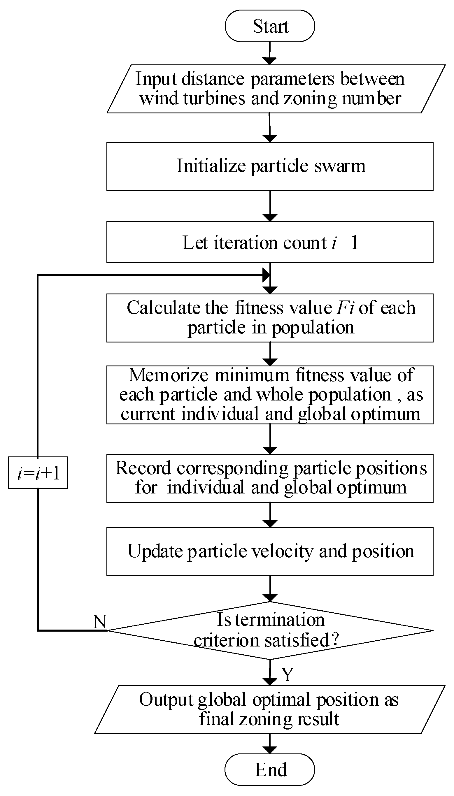
2.3. Optimal Zoning of Wind Farm Based on Improved DPSO

Assuming the wind farm is divided into $g$ clusters, $C=\left\{C_1,C_2,\dots ,C_g\right\}$, $\left|C_1\right|$,$\left|C_2\right|$,…, $\left|C_g\right|$ are defined as the number of samples contained in the corresponding cluster. Considering the cohesion within clusters and dispersion between clusters, the evaluation indexes of zoning are established as shown in Equations (10) and (11).

• Strong aggregation within zones

  $$f_{1a}=\frac{{\displaystyle {\sum }_{i\in C_a,j\in C_a}{d}_{ij}}}{\left|C_a\right|\cdot \left(\left|C_a\right|-1\right)},i\ne j$$

  (10)

  where: $f_{1a}$ represents convergence degree of wind turbines in zone $a$. The smaller the value of $f_{1a}$ is, the higher the aggregation degree in this zone.
• Strong dispersion between zones

  $$f_{2a}=\frac{{\displaystyle {\sum }_{i\in C_a}\left(\underset{C_b}{\min }\left\{\frac{{\displaystyle {\sum }_{j\in C_b,}{d}_{ij}}}{\left|C_b\right|}\right\}\right)}}{\left|C_a\right|},1\le b\le k,b\ne a$$

  (11)

  where: $f_{2a}$ represents separation degree from zone $a$ to other zones. The larger the value of $f_{2a}$ is, the more discrete this zone is from other zones.

Silhouette coefficient is a parameter used to evaluate clustering method model and clustering result itself, which combines the degree of aggregation and the degree of dispersion beneficially [19]. Based on the modeling idea of silhouette coefficient, the paper establishes an optimization zoning model combined with evaluation indexes, and the objective function is shown in Equation (12).

$$\min F=\frac{{\displaystyle \sum _{a=1}^k\left(\frac{f_{1a}-f_{2a}}{\max \left\{f_{1a},f_{2a}\right\}}+1\right)}}{k}$$

(12)

The value range of objective function $F$ is [0, 2]. The closer $F$ value is to 0, the better zoning result. Because the zoning result contains such information: stronger aggregation within zones and stronger dispersion between zones. Constraint conditions are shown in Equation (13):

$$\{\begin{array}{ll}g>1\hfill & \hfill \\ \left|C_a\right|>1,\hfill & a\in [1,g]\mathrm{and}a\in Z\hfill \\ \left|C_a\right|\le 0.8n,\hfill & a\in [1,g]\mathrm{and}a\in Z\hfill \end{array}$$

(13)

In order to solve optimal zoning model, an improved DPSO algorithm is adopted. The constraint conditions are processed by penalty function, that is, the penalty term is added to objective function, so that the particles which do not meet the constraint conditions cannot converge due to poor fitness. The solving process based on the improved DPSO algorithm is shown in Figure 1.

In order to improve the computational efficiency, on the basis of conventional DPSO algorithm, some improvements involving particle swarm initialization and particle position updating method are made as follows:

• Particle swarm initialization considering reverse learning and HC result

The initial particle swarm based on conventional DPSO algorithm is generally generated randomly and it is difficult to ensure uniform distribution of initial particle swarm in the solution space. In order to overcome the above defects, the improved DPSO algorithm considers adopting the method of reverse learning to initialize particle swarm [20,21,22], and the specific steps are as follows:

• Generate $\chi$ (particle number) initial spatial solutions in the feasible search domains randomly;

Suppose $g$ represents the number of clusters and $n$ is the dimension number of solution, which is the same as the number of wind turbines, the feasible solution of the $i^{\mathrm{th}}$ particle is expressed in Equation (14). All elements in $P_i$ satisfy $p_{ij}\in [1,g],p_{ij}\in Z(j=1,2,\dots ,n)$.

$$P_i=\left[p_{i1},p_{i2},\dots ,p_{in}\right]$$

(14)

• Calculate and generate the inverse solution of each initial solution;

The calculation of each dimensional component of the reverse solution is shown in Equation (15).

$$q_{ij}=1+g-p_{ij}$$

(15)

where: $q_{ij}$ represents the reverse solution in the $j^{\mathrm{th}}$ dimension of the $i^{\mathrm{th}}$ particle.

• The coarse clustering solution of HC algorithm in Section 2.1 is incorporated into the initial solution set of particle swarm.
• Based on the union set generated by the above random solutions, reverse solutions, and coarse clustering solution, the objective function value is calculated and solutions with lower value are selected preferentially to form the initial population.

2.

Particle position updating of DPSO algorithm

The updating of particle position is shown in Equations (16) and (17). The definition of relevant operators in the process of location updating is referred to [23].

$$U^{i+\mathbf{1}}=w{U}^i+o_{\mathbf{1}}(W_{\mathrm{pbest}}-W^i)+o_2(W_{\mathrm{gbest}}-W^i)$$

(16)

$$W^{i+1}=W^i+U^{i+1}$$

(17)

where: $U^i$ is the updated particle velocity of the i^th iteration; $W^i$ is the updated particle position of the i^th iteration; $W_{\mathrm{pbest}}$ is the current individual optimal particle position; $W_{\mathrm{gbest}}$ is the current global optimal particle position; $w$ is inertial weight; $o_1$ and $o_2$ are cognitive learning factor and social learning factor respectively, whose value range is [0, 1].

After solving optimal zoning model of a wind farm, which wind turbines belong to the same cluster can be determined. For the convenience of calculation, each cluster of wind turbines is processed into rectangular zone. The maximum distance between east and west and the maximum distance between north and south of each cluster are extended by 5% as the length and width of the rectangular zone respectively, and finally the specific scope of each rectangular wind zone can be obtained.

3. Micro Quantitative Siting of Met Mast Based on Grid Screening Method

3.1. Select Alternative Met Mast Positions by Gridding

When macro zoning of wind farm is completed, micro siting of met mast is carried out in each zone. In order to simplify calculation, each rectangular zone is divided into many grids and the shape of grids is square. In order to ensure that every possible location suitable for building met mast can be obtained as much as possible, the side length $L$ of grid should meet Equation (18), and the intersection points of grids are seen as the alternative wind monitoring points.

$$L=\min \left\{L_{ij}|i\in [1,n],j\in [1,n],i\ne j\right\}/\sqrt{2}$$

(18)

where: $L_{ij}$ is the actual distance between wind turbine $i$ and wind turbine $j$ in wind farm.

Then the optimal wind monitoring point should be determined among all alternative grid points. The best wind monitoring point should have a good representation of the wind resources in the corresponding wind zone. The representativeness of wind monitoring points is mainly based on the following principles: spatial consistency principle, representativeness principle of wind condition parameters in prevailing wind direction, and screening principle considering wind speed reduction caused by wake effect. Based on these principles, this paper establishes six indicators, namely horizontal distance from wind turbines, altitude difference from wind turbines, wind acceleration factor of prevailing wind direction, turbulence intensity of prevailing wind direction, inflow angle of prevailing wind direction, and wind speed reduction rate caused by wake effect. The screening process of alternative wind monitoring points is shown in Figure 2.

The wind condition parameters of prevailing wind direction and wind speed reduction rate caused by wake effect in each grid can be calculated by CFD software [24]. The steps of quantitative screening of alternative wind monitoring points are as follows.

Step 1: Exclude the alternative wind monitoring points within a distance away from wind turbines considering wake effect, as shown in Equation (19). The distance is equal to $\alpha$ times of rotor diameter.

$$R<\alpha D$$

(19)

where: $D$ is the rotor diameter; $R$ is the distance between the alternative wind monitoring points and wind turbines.

This screening index is mainly in response to standard [25]. Considering the wake effect of wind turbines, correction of free flow wind speed in front of wind turbines and so on, the value range of $\alpha$ is generally [2,4].

Step 2: Exclude alternative wind monitoring points whose altitude difference $\Delta h$ from wind turbines is more than reference value $H$, as shown in Equation (20).

$$\Delta h>H$$

(20)

Step 3: Calculate the average wind acceleration factor $\overline{u}$ of the prevailing wind direction at all wind turbines in the wind farm, and keep alternative wind monitoring points whose wind acceleration factor is within the fluctuation range of plus or minus 5% of the average, as shown in Equation (21).

$$u_i\in [0.95\overline{u},1.05\overline{u})],i=1,2,\dots ,m$$

(21)

where: $u_i$ is the wind acceleration factor in prevailing wind direction of i^th alternative wind monitoring point; $m$ is the number of alternative wind monitoring points reserved based on previous screening work.

Step 4: Calculate average turbulence intensity $\overline{l}$ in the prevailing wind direction of all alternative wind monitoring points reserved by above screening work, and keep the alternative wind monitoring points with turbulence intensity below $\overline{l}$, as shown in Equation (22).

$$l_i<\overline{l}$$

(22)

where: $l_i$ is the turbulence intensity in prevailing wind direction of the reserved i^th alternative wind monitoring point.

Step 5: Calculate average $\overline{\epsilon }$ of absolute value of inflow angle in prevailing wind direction of all alternative wind monitoring points reserved by above screening work, and keep the alternative wind monitoring points with absolute value of inflow angle below $\overline{\epsilon }$, as shown in Equation (23).

$${\epsilon }_i<\overline{\epsilon }$$

(23)

where: ${\epsilon }_i$ is the absolute value of inflow angle in prevailing wind direction of the reserved i^th alternative wind monitoring point.

Step 6: Calculate average wind speed reduction rate $\overline{\omega }$ of all alternative wind monitoring points reserved by above screening work, and keep the alternative wind monitoring points with wind speed reduction rate below $\overline{\omega }$, as shown in Equation (24).

$${\omega }_i<\overline{\omega }$$

(24)

where: ${\omega }_i$ is the wind speed reduction rate caused by wake effect of the reserved i^th alternative wind monitoring point.

3.2. Micro Siting Evaluation of Met Mast in Wind Farm

The siting index is established to select the best position point of met mast from above finally reserved alternative wind monitoring points. Average wind speed distribution provides important information of wind resources. Meanwhile, the Weibull distribution, represented by shape parameters $k$ and scale parameters $c$, is the most common wind speed distribution. The Weibull distribution is expressed by Equation (25).

$$P(v)=\frac{k}{c}{(\frac{v}{c})}^{k-1}{e}^{-{(\frac{v}{c})}^k}$$

(25)

where: $P(v)$ is the probability density of wind speed distribution.

As met mast should be representative of the wind resources in wind farm as much as possible, the average wind speed distribution of met mast should be as consistent as possible with the average wind speed distribution of wind turbines. That is, Weibull distribution parameters of met mast should be as consistent as possible with average Weibull distribution parameters of wind turbines in each wind zone.

In order to evaluate the representativeness of the reserved alternative wind monitoring points in the corresponding zone, the evaluation index $Y$ of met mast siting is defined by Equation (26).

$$Y=1-\left(\frac{\left|v_{\mathrm{ave}}-v_{\mathrm{mo}}\right|}{v_{\mathrm{ave}}}+\frac{\left|k_{\mathrm{ave}}-k_{\mathrm{mo}}\right|}{k_{\mathrm{ave}}}+\frac{\left|c_{\mathrm{ave}}-c_{\mathrm{mo}}\right|}{c_{\mathrm{ave}}}\right)/3$$

(26)

where: $v_{\mathrm{mo}}$, $k_{\mathrm{mo}}$, and $c_{\mathrm{mo}}$ are respectively the wind speed, the shape parameter, and the scale parameter of the alternative wind monitoring points; $v_{\mathrm{ave}}$, $k_{\mathrm{ave}}$, and $c_{\mathrm{ave}}$ are respectively the mean of wind speed, the mean of shape parameter, and the mean of scale parameter of all wind turbine positions.

The value of index $Y$ is within the range of [0, 1]. The closer the $Y$ value of the alternative wind monitoring point is to 1, the more suitable its location is for building a met mast.

In summary, the research framework of this paper is shown in Figure 3.

4. Simulation Verification

An island wind farm in Zhejiang province is selected. The wind farm is located in the range of east longitude ${121}^{\circ }{55}^{\prime }{24}^{″}\sim {121}^{\circ }{57}^{\prime }{44}^{″}$ and north latitude ${29}^{\circ }{47}^{\prime }{17}^{″}\sim {29}^{\circ }{48}^{\prime }{12}^{″}$, with altitude of 0~255 m. There are 17 wind turbines in the wind farm and the prevailing wind direction is about ${300}^{\mathrm{o}}$. The topography of the wind farm is shown in Figure 4.

Based on historical wind speed information of all wind turbine positions, the REOF method is used to analyze the spatial distribution characteristics of wind speed.

Table 1. The Variance Contribution rate and Cumulative Variance Contribution Rate of the First Two Feature Vectors of Regional Wind Speed Based on EOF and REOF.

Serial Number	EOF Variance Contribution Rate	REOF Variance Contribution Rate	Cumulative Variance Contribution Rate
1	96.27%	74.93%	/
2	3.68%	25.02%	99.95%

shows the variance contribution rate and cumulative variance contribution rate of the first two feature vectors of wind speed based on EOF and REOF. The cumulative variance contribution rate of the first two feature vectors is 99.95%, i.e., the first two feature vectors can effectively represent the overall characteristics of wind speed changes in wind farms. After rotation, the variance contribution of each load vector is more evenly distributed than before rotation. The total variance contribution does not change, and the rotation effect is significant. However, the variance contribution rate of the first feature vector is 74.93%, which still account for a large proportion of the total variance. It implies that the first vector takes majority responsibility for representing wind speed characteristics of wind farm. According to the spatial distribution information of rotating load vector field obtained by REOF, the corresponding heat map is made, as shown in Figure 5. It is obvious that there are two load centers with significantly different wind speed characteristics in wind farms. One is mainly concentrated at #7 wind turbine, and the other load center is mainly concentrated at #1 wind turbine.

Based on location information (latitude, longitude and altitude) of wind turbines, HC algorithm is used to draw hierarchical pedigree diagram, as shown in Figure 6. Combined with the REOF information, it can be preliminarily judged the wind farm is suitable to be divided into two zones, and coarse clustering result of wind turbines is obtained based on the pedigree diagram.

Inertia weight coefficient w = 0.7 and the parameters o₁ = 0.2, o₂ = 0.3 in DPSO algorithm are taken to calculate the optimal zoning result. Meanwhile, DBSCAN zoning method is compared with DPSO method and respective result is shown in Figure 7 (Wind turbines with the same symbol are in the same wind zone in Figure 7b–d). Although DBSCAN as a classical clustering algorithm can automatically determine zoning number, the output zoning results are different when input parameters such as cluster density threshold d are set to different values. In this paper, two DBSCAN results when zoning number is 2 are selected and presented. As can be seen from Figure 7, under different d values, #8, #9, #10, #15, #16, and #17 wind turbines (the serial number of wind turbines is shown in Figure 4) are divided into completely different zone, indicating that the final zoning result of DBSCAN is very sensitive to parameter selection.

For clustering zoning without label, silhouette coefficient is generally considered to objectively evaluate zoning results [19]. The value range of silhouette coefficient is [–1, 1], the closer it is to 1, the better zoning effect is. Comparison of silhouette coefficient based on DBSCAN and DPSO algorithm is shown in

Table 2. Comparison of silhouette coefficient based on DBSCAN and DPSO algorithm.

Serial Number	DBSCAN Algorithm d = 3	DBSCAN Algorithm d = 4	DPSO Zoning
Silhouette coefficient	0.5240	0.6163	0.6285

. It can be seen that the silhouette coefficient of the DPSO zoning result is the largest, which proves that the zoning result is the optimal objectively. In addition, when d = 4, the DBSCAN zoning result is close to DPSO zoning, and the corresponding silhouette coefficient is suboptimal. The results of two zoning methods mirror each other to some extent, which further verifies the rationality of DPSO zoning.

Compared with DBSCAN algorithm, DPSO zoning has the following advantages:

(1)

In DBSCAN algorithm, parameters are very important, which is difficult to select and has a great influence on zoning results. However, the parameter selection of DPSO zoning has no influence on final optimization results, but only plays a role in the calculation efficiency. Moreover parameter selection is relatively simple.

(2)

In the DBSCAN algorithm, different input parameters lead to different zoning results. Every result needs to be evaluated by a silhouette coefficient. The evaluation work is relatively heavy because of lots of repetitive work, and the optimality of the evaluated zoning result cannot be guaranteed because of the diversity of input parameters. However, the DPSO zoning model takes the evaluation index into account, which makes evaluation work easier. Moreover, the final optimal zoning result is presented directly by a clear and concise algorithm. The final zoning result of this wind farm is shown in Figure 8.

On the other hand, according to the REOF heat map, the first load center concentrated at #7 wind turbine corresponds to No. 2 wind zone in DPSO zoning result. The second load center concentrated at #1 wind turbine corresponds to No.1 wind zone. The reliability of DPSO zoning results is verified.

To further verify the superiority of the improved DPSO algorithm, Zhushan wind farm in Zhejiang province with 50 wind turbines is selected. The terrain and DPSO zoning result are shown in Figure 9 and Figure 10 (Wind turbines with the same symbol are in the same wind zone in Figure 10b). It can be seen that Zhushan wind farm covers a large area and optimal zoning result is obviously related to the geographical location proximity between wind turbines, in line with practical experience. The convergence curves of the algorithm applied to island wind farm and Zhushan wind farm are shown in Figure 11. It can be found that:

(1)

The convergence speed of the improved DPSO algorithm is faster than that of the conventional DPSO algorithm.

(2)

In the island wind farm, when converging, there is a difference of about seven iterations between improved DPSO and conventional DPSO algorithm. Meanwhile, in the larger Zhushan wind farm, there is a difference of almost 70 iterations between improved DPSO and conventional DPSO algorithm. That is to say, the convergence speed of the improved DPSO algorithm is improved more obviously for wind farms with larger scale.

The results show that the improved DPSO algorithm can effectively improve the computational efficiency, and the larger the data scale is, the more obviously the efficiency of algorithm improves.

Micro siting of met mast is carried out in two zones of the island wind farm. The design of relevant parameters is referred in [26]. Firstly, Windsim software is used to simulate spatial wind flow distribution by the CFD numerical method. Wind condition parameters in the prevailing wind direction, including wind acceleration factor, turbulence intensity, inflow angle, and reduced wind speed considering wake effect, are obtained by gridding the calculation of the target area of the wind farm. Next based on obtained grid information, alternative wind monitoring points are screened out according to micro quantitative siting strategy of met mast. Finally, the optimal locations of met mast in each zone are obtained based on the calculation of siting evaluation index. The screening results of alternative wind monitoring points are shown in

Table 3. Screening results of alternative wind monitoring points.

	Alternative Wind Monitoring Points	Index	Selection of Wind Monitoring Points
No.1 wind zone	P1 P2	0.923761 0.825439	P1
No.2 wind zone	P3 P4 P5	0.905465 0.796873 0.846572	P3

. The optimal location of wind monitoring point is shown in Figure 12. The two optimal locations of met masts in respective zones are relatively consistent with the above two load centers based on REOF method, which verifies the representativeness of met mast in final selected position.

To further prove the effectiveness of the proposed micro siting method, the met mast positions determined by proposed method (met mast at points P₁, P₃, corresponding longitude, latitude are respectively 121°55’49.2″ E, 29°47′18.2″ N/121°56′50.3″ E, 29°47′13.4″ N) and common method based on engineering experience in [14] (met mast at points P₆, P₇, corresponding longitude, latitude are respectively 121°56′10.1″ E, 29°47′80.3″ N/121°56′59.6″ E, 29°48′17.4″ N) are respectively used as CFD simulation inputs, and estimated results and errors regarding the annual power generation of wind farms are shown in

Table 4. Annual energy production and error analysis of wind farm.

Input Data	Average Annual Power Generation/(104 kW·h)	Relative Error/%
	12,540.32 (actual measured power generation)
(P1, P3)	12,314.59	−1.8
(P6, P7)	12,101.41	−3.5
P1	11,449.31	−8.7
P3	13,079.55	+4.3
P6	11,474.39	−8.5
P7	13,154.80	+4.9

. It can be seen that taking met mast positions (P₁, P₃) as input, the error of estimated power generation is the smallest. In addition, the error of estimated power generation with two met masts is smaller, compared with one met mast. It is indicated that two met masts are more representative for wind resources of the island wind farm. The reliability of the proposed method is verified to some extent.

5. Conclusions

In this paper, a method for the optimal layout of met mast in the wind farm is proposed. Firstly, a representative wind zone scope and the number of met mast are determined by macro zoning of wind farm. Then, a micro quantitative siting strategy is proposed and the optimal layout evaluation index is established to realize micro siting of met mast in each wind zone. The main conclusions are drawn as follows:

(1)

The proposed optimal zoning method based on discrete particle swarm optimization provides a new zoning idea, which can provide a reliable zoning result for wind farms more directly and quickly compared with general zoning methods, such as the density based spatial clustering of applications with noise algorithm method.

(2)

In the studied cases, the selected met mast position based on the proposed micro quantitative siting method is proven to be more accurate and representative by the test of wind farm power generation estimation, compared with the traditional qualitative analysis method.

The optimal layout method for met mast proposed in this paper has certain practical applicability, especially for wind farms with large scale or complex terrain. It can help to obtain more accurate data regarding wind resources, which means a lot for wind farm operation. In future work, the layout evaluation index will be further discussed and designed considering different functions of met mast, which will serve to improve micro siting work of met mast.

References

1. Yao, J.; Yao, F. Status quo, development and utilization efficiencies of wind power in China. Processes 2021, 9, 2133. [Google Scholar] [CrossRef]
2. Liu, Y.; Yang, J.; Jiang, C.; Niu, S.; Li, H.; Chen, S. Review on met mast site selection methods in grid-connected wind farm. In Proceedings of the 2019 IEEE 3rd International Electrical and Energy Conference (CIEEC), Beijing, China, 7–9 September 2019; pp. 1134–1137. [Google Scholar]
3. Gao, Z.; Liu, X. An overview on fault diagnosis, prognosis and resilient control for wind turbine systems. Processes 2021, 9, 300. [Google Scholar] [CrossRef]
4. Fan, G.; Wang, Y.; Yang, B.; Zhang, C.; Fu, B.; Qi, Q. Characteristics of wind resources and post-project evaluation of wind farms in coastal areas of Zhejiang. Energies 2022, 15, 3351. [Google Scholar] [CrossRef]
5. Dong, Y.; Zhang, L.; Liu, Z.; Wang, J. Integrated forecasting method for wind energy management: A case study in China. Processes 2020, 8, 35. [Google Scholar] [CrossRef]
6. Jangamshetti, S.; Ran, V. Optimum siting of wind turbine generator. IEEE Trans. Energy Convers. 2001, 16, 8–13. [Google Scholar] [CrossRef]
7. Bebi, E.; Alcani, M.; Malka, L.; Leskoviku, A. An evaluation of wind energy potential in Topoja area, Albania. Sci. Bus. Soc. 2022, 7, 21–25. [Google Scholar]
8. Bailey, B.H. Wind Resource Assessment Handbook: Fundamentals for Conducting a Successful Monitoring Program; National Renewable Energy Laboratory (NREL): Golden, CO, USA, 1997; pp. 23–24. [Google Scholar]
9. Sun, S.; Liu, S.; Liu, J.; Schlaberg, H.I. Wind field reconstruction using inverse process with optimal sensor placement. IEEE Trans. Sustain. Energy 2019, 10, 1290–1299. [Google Scholar] [CrossRef]
10. Khan, K.S.; Tariq, M. Wind resource assessment using SODAR and meteorological mast—A case study of Pakistan. Renew. Sust. Energ. Rev. 2018, 81, 2443–2449. [Google Scholar] [CrossRef]
11. Han, P.; Xia, Y.; Zhang, Y.; Luo, K. Equivalent model of wind farm based on DBSCAN. In Proceedings of the 2017 IEEE Innovative Smart Grid Technologies-Asia (ISGT-Asia), Auckland, New Zealand, 4–7 December 2017; pp. 1–6. [Google Scholar]
12. Bechrakis, D.; Sparis, P. Correlation of wind speed between neighboring measuring stations. IEEE Trans. Energy Convers. 2004, 19, 400–406. [Google Scholar] [CrossRef]
13. Yang, J.Y.; Woo, Y.M.; Sheng, K.; Tang, Y.H. Research on the met mast siting used in post assessment of mountain wind farm. In Proceedings of the World Wind Energy Conference, Shanghai, China, 7–9 April 2014; pp. 443–447. [Google Scholar]
14. Zhang, H. Wind Resources and Micro-Location; China Machine Press: Beijing, China, 2013; pp. 42–43. [Google Scholar]
15. Sun, S.; Liu, S.; Chen, M.; Guo, H. An optimized sensing arrangement in wind field reconstruction using CFD and POD. IEEE Trans. Sustain. Energy 2020, 11, 2449–2456. [Google Scholar] [CrossRef]
16. Terciyanlı, E.; Demirci, T.; Küçük, D.; Saraç, M.; Çadırcı, I.; Ermiş, M. Enhanced nationwide wind-electric power monitoring and forecast system. IEEE Trans. Industr. Inform. 2014, 10, 1171–1184. [Google Scholar] [CrossRef]
17. Wu, J.; Chen, Y.; Guo, P.; Wang, X.; Hu, X.; Wu, M. Sea surface wind speed retrieval based on empirical orthogonal function analysis using 2019–2020 CYGNSS data. IEEE Trans. Geosci. Remote Sens. 2022, 60, 5803213. [Google Scholar] [CrossRef]
18. Tso, W.; Demirhan, C.; Heuberger, C.; Powell, J.; Pistikopoulos, E. A hierarchical clustering decomposition algorithm for optimizing renewable power systems with storage. Appl. Energy 2020, 270, 115190. [Google Scholar] [CrossRef]
19. Dinh, D.T.; Fujinami, T.; Huynh, V.N. Estimating the optimal number of clusters in categorical data clustering by silhouette coefficient. In International Symposium on Knowledge and Systems Sciences; Springer: Singapore, 2019; pp. 1–17. [Google Scholar]
20. Cao, Y.; Zhang, H.; Li, W.; Zhou, M.; Zhang, Y.; Chaovalitwongse, W.A. Comprehensive learning particle swarm optimization algorithm with local search for multimodal functions. IEEE Trans. Evol. Comput. 2019, 23, 718–731. [Google Scholar]
21. Bangyal, W.H.; Nisar, K.; Ibrahim, A.A.; Haque, M.R.; Rodrigues, J.J.; Rawat, D.B. Comparative analysis of low discrepancy sequence-based initialization approaches using population-based algorithms for solving the global optimization problems. Appl. Sci. 2021, 11, 7591. [Google Scholar] [CrossRef]
22. Ashraf, A.; Pervaiz, S.; Haider Bangyal, W.; Nisar, K.; Ibrahim, A.A.; Rodrigues, J.J.; Rawat, D.B. Studying the impact of initialization for population-based algorithms with low-discrepancy sequences. Appl. Sci. 2021, 11, 8190. [Google Scholar] [CrossRef]
23. Guo, Z.; Liang, Y.; Bian, X.; Wang, D. Multi objective optimization for arrangement of the asymmetric-paths winding based on improved discrete particle swarm approach. IEEE Trans. Energy Convers. 2018, 33, 1571–1578. [Google Scholar] [CrossRef]
24. Iranzo, A. CFD applications in energy engineering research and simulation: An introduction to published reviews. Processes 2019, 7, 883. [Google Scholar] [CrossRef]
25. National Power Dispatch and Communication Center. Functional Specification of Wind Power Forecasting System: Q/GDW 10588-2015; State Grid Corporation of China: Beijing, China, 2015. [Google Scholar]
26. Zhang, X. The Research and Application on Optimal Site Selection of a Met Mast in a Large-scale Interconnected Wind Farm; North China Electric Power University: Beijing, China, 2018. [Google Scholar]
Figure 1. Improved DPSO algorithm.
Processes 10 01708 g001
Figure 2. Location screening process of alternative met mast.
Processes 10 01708 g002
Figure 3. The research framework of this paper.
Processes 10 01708 g003
Figure 4. The topography of island wind farm.
Processes 10 01708 g004
Figure 5. Heat map of load vector field spatial distribution based on REOF.
Processes 10 01708 g005
Figure 6. Hierarchical pedigree diagram of wind turbines clustering process.
Processes 10 01708 g006
Figure 7. Comparison of zoning results based on DBSCAN and DPSO algorithm.
Processes 10 01708 g007
Figure 8. Zoning result of the island wind farm.
Processes 10 01708 g008
Figure 9. The topography of Zhushan wind farm.
Processes 10 01708 g009
Figure 10. Optimal zoning result of Zhushan wind farm.
Processes 10 01708 g010
Figure 11. Convergence curves of discrete particle swarm optimization algorithm.
Processes 10 01708 g011
Figure 12. Optimal location of wind monitoring point.
Processes 10 01708 g012