Abstract
Liquified natural gas (LNG) manipulator arms have been widely used in natural gas transportation. However, the automatic docking technology of LNG manipulator arms has not yet been realized. The first step of automatic docking is to identify and locate the target and estimate its pose. This work proposes a petroleum pipeline interface recognition and pose judgment method based on binocular stereo vision technology for the automatic docking of LNG manipulator arms. The proposed method has three main steps, including target detection, 3D information acquisition, and plane fitting. First, the target petroleum pipeline interface is segmented by using a color mask. Then, color space and Hu moment are used to obtain the pixel coordinates of the contour and center of the target petroleum pipeline interface. The semi-global block matching (SGBM) algorithm is used for stereo matching to obtain the depth information of an image. Finally, a plane fitting and center point estimation method based on a random sample consensus (RANSAC) algorithm is proposed. This work performs a measurement accuracy verification experiment to verify the accuracy of the proposed method. The experimental results show that the distance measurement error is not more than 1% and the angle measurement error is less than one degree. The measurement accuracy of the method meets the requirements of subsequent automatic docking, which proves the feasibility of the proposed method and provides data support for the subsequent automatic docking of manipulator arms.
1. Introduction
The liquified natural gas (LNG) manipulator arm is critical equipment for loading and unloading petroleum and other fluids at ports. One of the daily tasks of the dock workers is to connect the LNG manipulator arm with the pipeline interface located on the ship. However, the traditional manual towing methods are not only time-consuming and labor-intensive, but they also have various potential safety hazards. For instance, when the epidemic situation was severe, frequent contact with foreign ships increased the risk of infections. In addition, with the intensification of the aging population, the labor cost is continuously increasing. Therefore, realizing an unmanned docking control of the LNG manipulator arm improves the safety and production efficiency of port production.
As compared with manual methods, the machine vision technologies have high efficiency and do not require the physical contact. Moreover, as compared with traditional surveying and mapping methods, the machine vision technologies have high flexibility due to a smaller number of steps required for setting markers. Che et al. [1] proposed a high-precision and contactless method for measuring the parts assembly clearance by performing image processing based on machine vision. Gu et al. [2] set up a visual measurement system to obtain the drilling bit wear characteristics and evaluated its wear condition. Millara et al. [3] built a system based on laser emitters and cameras for dimensional quality inspection during the manufacturing process of railway tracks. Li et al. [4] proposed a turning control algorithm based on monocular vision vehicle turning path prediction. The algorithm estimates the cornering trajectory of a vehicle based on the vehicle’s front axle length and front-wheel adjustment data.
The machine vision detection technologies have been applied in various fields, such as agriculture, manufacturing industry, and medical industry. Abhilash et al. [5] developed a closed-loop machine vision system for the wire electrical discharge machining (EDM) process control. This system successfully predicts the wire breakage by monitoring the severity of the wire wear. Lin et al. [6] used machine vision technology for detecting the surface quality of fluff fabric. It detects the fabric defects and pilling by establishing qualitative and quantitative evaluation models. Ropelewska et al. [7] converted the images of beetroots to different color channels and used models based on textures selected for each color channel to discriminate the raw and processed beetroots. Nawar et al. [8] proposed a prototype based on color segmentation with a SVM classifier to recognize the skin problems quickly at a low cost. Sung et al. [9] developed an automatic grader for flatfish using machine vision. Keenan et al. [10] proposed an objective grading system using automated machine vision for solving the problem, i.e., the histological grading of cervical intraepithelial neoplasia (CIN) is subjective and has poor reproducibility. Liu et al. [11] established a semantic segmentation network that is applied to the scene recognition in the warehouse environment. Yang et al. [12] proposed a detection method of bubble defects on tire surfaces based on line lasers and machine vision to eliminate driving dangers caused by tire surface bubbles. Lin et al. [13] used the machine vision and artificial intelligence algorithms to rapidly check the degree of cooking of foods to avoid the over-cooking of foods. Im et al. [14] proposed a large-scale Object-Defect Inspection System based on Regional Convolutional Neural Network (R-CNN; RODIS) to detect the defects of the car side-outer.
In addition to identifying the target pipeline interface, the docking also needs to measure the distance and relative pose relationship between the target and the manipulator arm. Therefore, it is necessary to use binocular stereo vision for obtaining the depth information of the target. Please note that the stereo vision technology has a wide range of applications in many fields. Tuan et al. [15] proposed an approach based on deep learning and stereo vision to determine the concrete slumps in the outdoor environments. Afzaal et al. [16] developed a method based on stereo vision for estimating the roughness formed on the agricultural soils, and the soil till quality was investigated by analyzing the height of plow layers. Kardovskyi et al. [17] developed an artificial intelligence-based quality inspection model (AI-QIM) that uses the mask region-based convolutional neural network (Mask R-CNN) to perform instance segmentation of steel bars and generate information regarding steel bar installation by using stereo vision. Gunatilake et al. [18] proposed a mobile robotic sensing system that can scan, detect, locate, and measure the internal defects of a pipeline by generating three-dimensional RGB depth maps based on stereo camera vision combined with infrared laser profiling unit.
After completing the stereo matching to obtain the point cloud, it is often necessary to process it according to the requirements; for example, plane fitting is required in this work. Some data analysis methods, such as principal component analysis (PCA) [19], independent component analysis (ICA) [20], and support vector machine (SVM) [21,22], are reviewed in [23]. Li et al. [24] developed an accurate plane fitting method for a structured light (SL)-based RGB-D sensor and proposed a new cost function for a RANSAC-based plane fitting method. Hamzah et al. [25] presented an improvement in the disparity map refinement stage by using an adaptive least square plane fitting technique to increase the accuracy during the final stage of stereo matching algorithm. Yu et al. [26] proposed a cylinder fitting method with incomplete three-dimensional point cloud data based on the cutting plane due to the influence of occlusion and noise. Kermarrec et al. [27] used the residuals of the least-squares surface approximation of TLS point clouds for quantifying the temporal correlation of TLS range observations.
The identification and positioning of the petroleum pipeline interface and the judgment of the orientation of the interface are the primary links for accomplishing the automatic docking of the manipulator arm. Please note that these are the most important links in the entire docking process. This work explores an efficient, accurate, and flexible method based on binocular vision technology for the identification of petroleum pipeline interface and detecting its orientation according to the requirements of the docking of manipulator arm. In this work, the images are preprocessed, and the region of the petroleum pipeline interface is extracted by transforming the color space and setting the threshold of the image channels. The 2D coordinates of the interface’s inner contour and the center are obtained by the function, i.e., findContours, available in OpenCV. The 3D coordinates of the interface’s contour are obtained by using the binocular stereo vision. Then, the plane fitting algorithm based on the RANSAC algorithm [28,29] is used to fit the 3D coordinates of the interface’s contour. The algorithm based on RANSAC performs better than the least-squares-based methods presented in [25,27], when there is a presence of abnormal samples. Finally, based on the space plane equation, the orientation of the petroleum pipeline interface (the normal vector of the fitting plane) and the 3D coordinates of the interface’s center are obtained. In this work, machine vision technology is used to automatically detect and identify the position and direction of the petroleum pipeline interface, which provides basic data for the subsequent automatic docking of the LNG manipulator arm. Vongbunyong et al. [30] presented an implementation of a precise docking maker technique for the localization of robots. This technique is based on Lidar sensor and setting geometrical markers. As compared with the method presented in [30], the methods based on machine vision are more flexible and do not require special markers.
2. Manipulator Arm Docking Action
Figure 1 presents the unloading arm docking scenario. The binocular camera is installed above the end effector of the manipulator arm. The manipulator arm automatically moves to the preset area when performing the docking action. Then, the camera captures the petroleum pipeline interface and transmits the images back to the computer. After the computer receives the images, it runs the recognition algorithm to read the position coordinates and orientation of the target petroleum pipeline interface. Subsequently, this information is converted into action commands to control the movement of the manipulator arm. Finally, the manipulator arm docks with the petroleum pipeline interface. This work mainly studies the identification, positioning, and pose judgment of the target. Figure 2 presents the flowchart of the process.
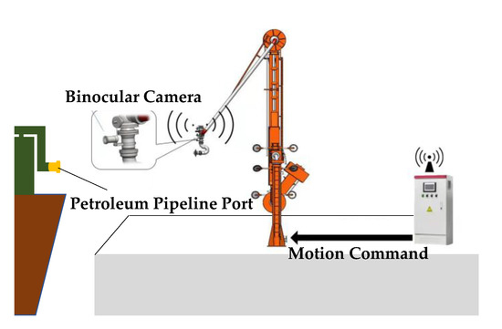
Figure 1.
The schematic diagram of unloading arm docking scenario.
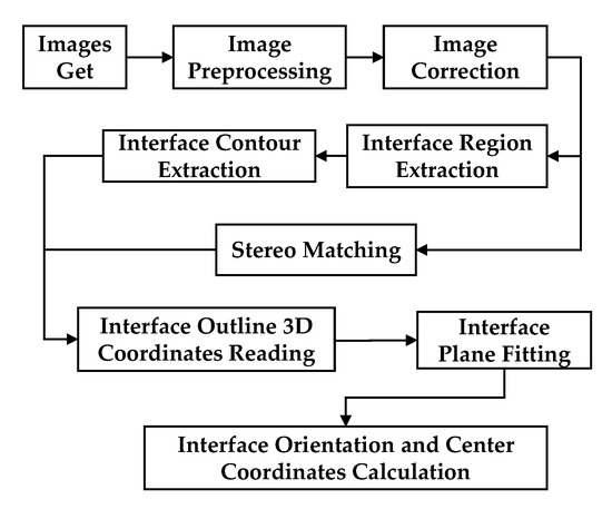
Figure 2.
The flowchart of the proposed vision system.
3. Petroleum Pipeline Interface Identification
3.1. Segmentation and Extraction of Petroleum Pipeline Interface
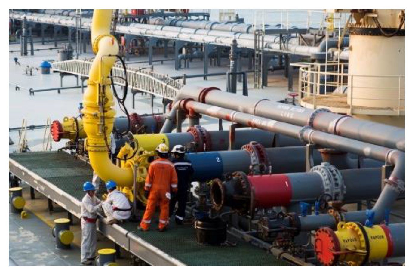
It is noteworthy that in actual production, the pipeline interface is often marked with different colors as compared to the background in order to facilitate the staff to identify the purpose of each pipeline and avoid the occurrence of safety problems. Figure 3 shows the actual manipulator arm docking scenario.
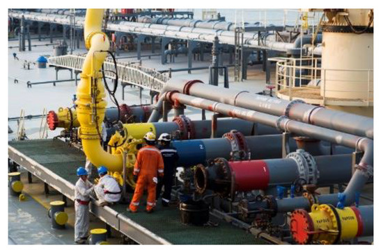
Figure 3.
An actual manipulator arm docking scenario.
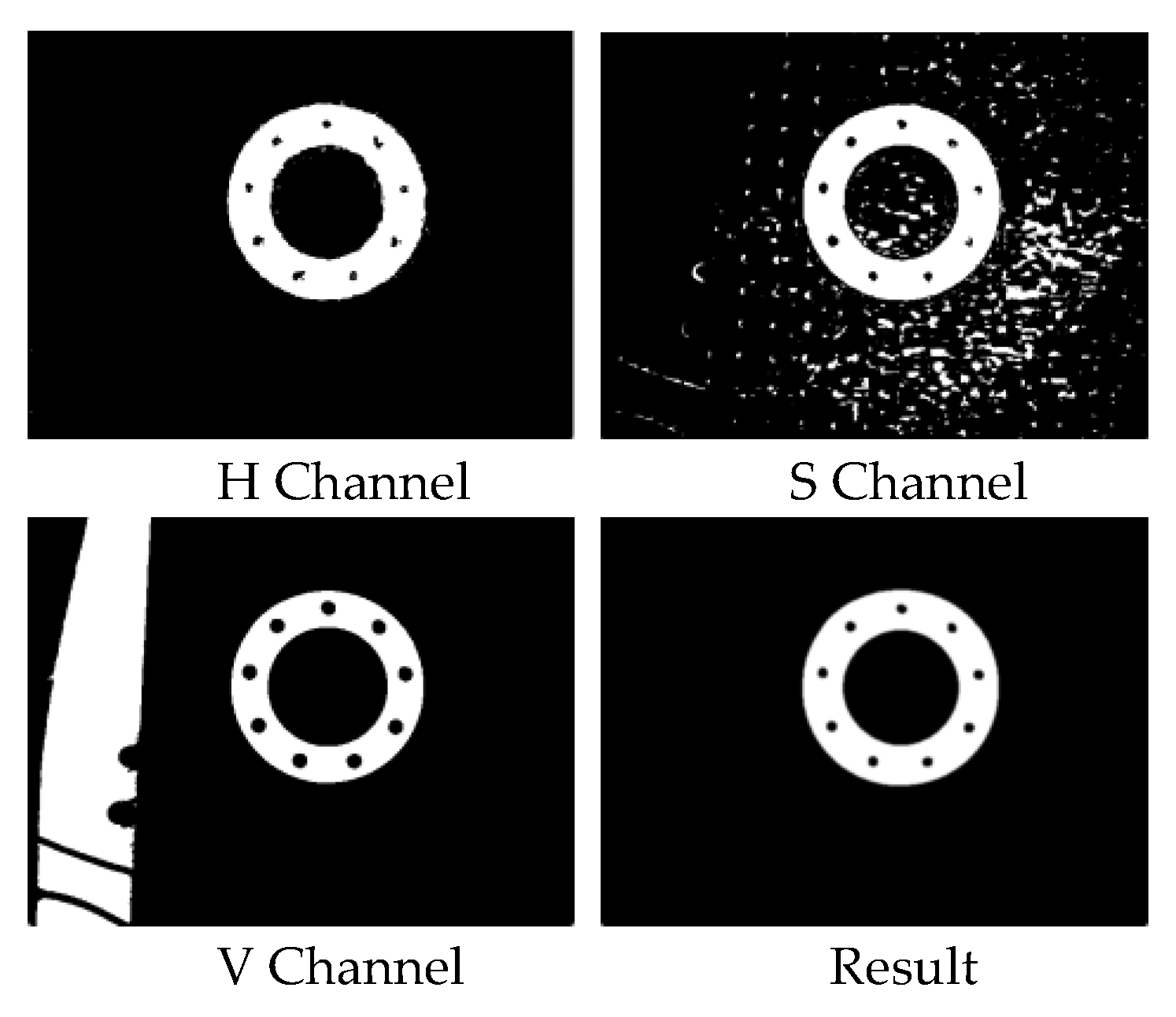
The choice of color space [31] is particularly critical when performing image segmentation. The RGB images are acquired by the camera. In order to filter out a certain color from the RGB color space, the values of R, G, and B channels are adjusted. However, this process is complex and abstract, and it is impossible to intuitively judge the correctness of the setting parameters. Therefore, the RGB color space is transformed to HSV color space [32,33]. In HSV color space, H represents hue and denotes the type of color, S represents the saturation and denotes the depth of a color, and V represents the lightness and denotes the brightness of a color. Therefore, the desired area can be roughly extracted by appropriately selecting the value of hue (H) when using the HSV color space for performing image segmentation. Then, based on the actual situation, the interference areas are further filtered by setting the appropriate values of saturation (S) and brightness (V). Finally, the desired area is extracted. Figure 4 shows the regions extracted from different image channels and the final extraction result after thresholding the HSV image.

Figure 4.
The extraction results of the petroleum pipeline interface.
3.2. Outline Extraction of Petroleum Pipeline Interface
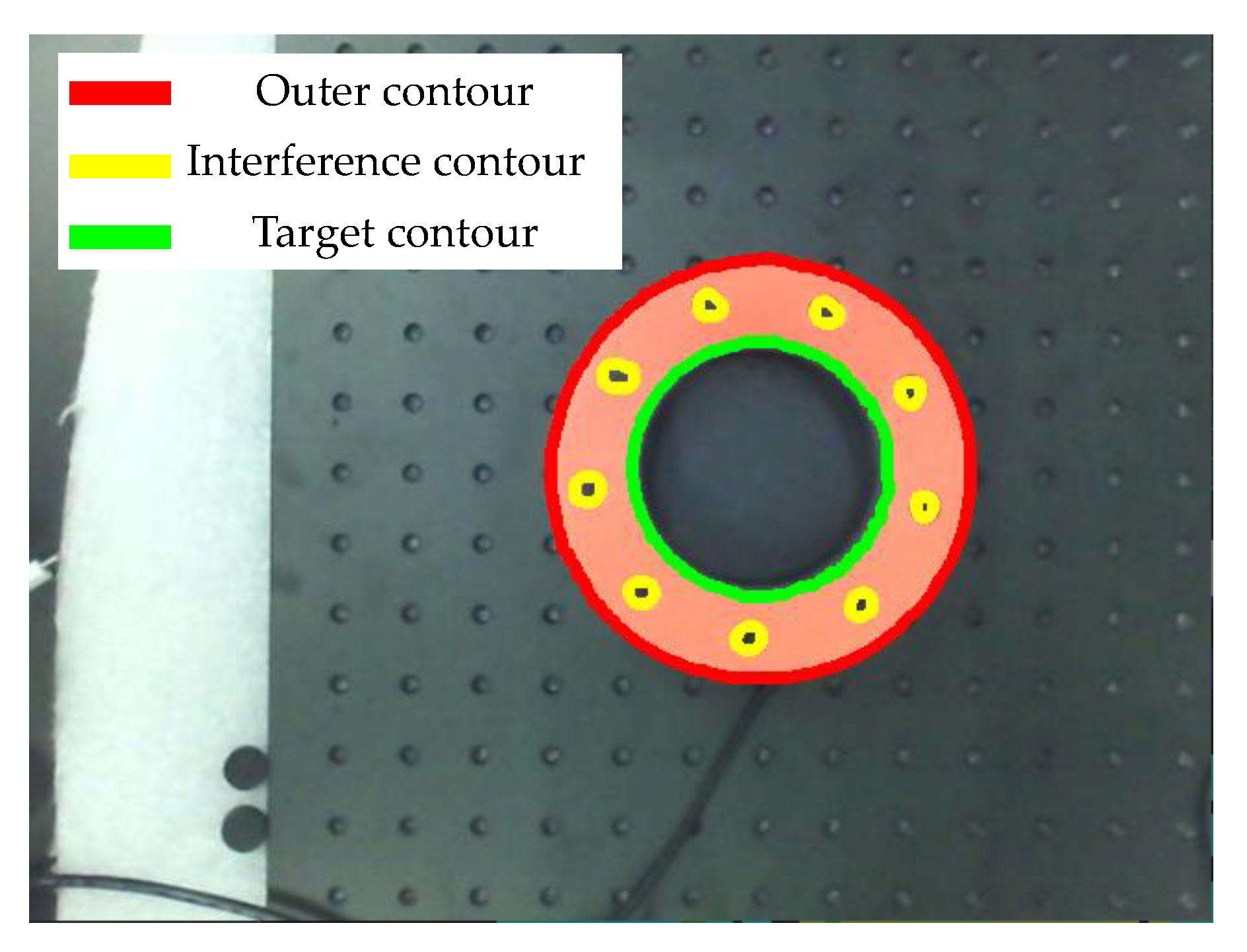
The contour information of the images can be easily obtained by using the contour search function findContours available in OpenCV [34,35,36]. However, there are many false contours retrieved by this function. Therefore, it is necessary to screen the retrieved contours. The interface area after image segmentation based on color space presents an irregular outer contour when the camera angle is oblique to the pipeline. Please note that the irregular contours cannot be used to detect the center position of the petroleum pipeline interface. Therefore, the inner contour of the petroleum pipeline interface should be extracted. The RETR_TREE mode of findContours filters out the inner contours by observing the parameter hierarchy. There are holes for fixing around the flange of the interface. The contours of these holes also belong to the inner contours, which interfere with the recognition result. Figure 5 shows different contours of the 3D printing flange model. Therefore, all the retrieved inner contours are sorted by size, and the largest contour is selected as the target contour.

Figure 5.
Different contours of the 3D printing flange model.
3.3. Calculation of Petroleum Pipeline Interface’s Center
The petroleum pipeline interface is a circular interface. When a camera is not facing the interface, it appears elliptical in the 2D projection of the imaging plane. Please note that the circle and ellipse are centrosymmetric figures, and the center of the centrosymmetric figure coincides with the center of gravity. Therefore, Hu moment [37,38,39] is used to determine the center of the interface. Let f (x, y) represent the gray value at pixel coordinate (x, y), then the zero order moment, first order moment, and the center of the graph are mathematically expressed by (1), (2), and (3), respectively.
The extraction result of the color space is a binarized image. The graph center coordinate calculated by using the Hu moment is regarded as the center coordinate of the area surrounded by the contour points.
After extracting the contour of the petroleum pipeline interface and calculating the center coordinates, we project them on the original image. The corresponding result is shown in Figure 6.
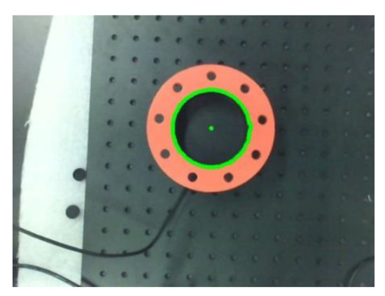
Figure 6.
The extraction results of contour and center coordinates.
4. Stereo Vision Ranging System
4.1. The Principle of Target 3D Coordinate Acquisition
In order to obtain the 3D coordinates by using the binocular stereo vision, two cameras are first used to capture the same object from different positions to obtain two images. Then, the imaging deviation of the target feature points on the two images is calculated based on the principle of stereo matching and similar triangles. Consequently, the depth information of the feature points is obtained, and the 3D space coordinates are calculated. The principle of binocular stereo vision is shown in Figure 7.
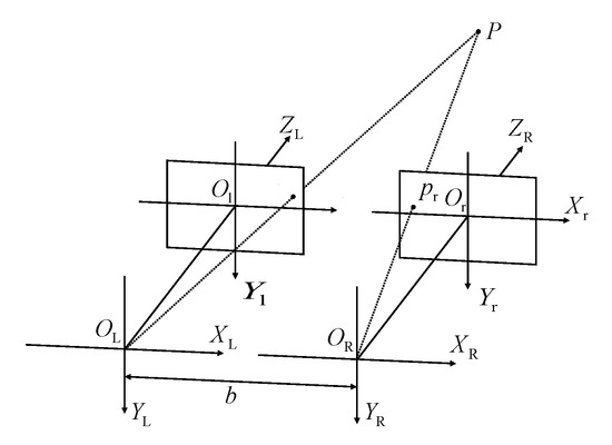
Figure 7.
The schematic diagram of ideal binocular stereo vision.
In Figure 7, f denotes the focal length of the left and right cameras, OL and OR are the optical centers of the left and right cameras, respectively, and OLZL and ORZR are the optical axes of the left and right cameras, respectively. In the ideal binocular stereo vision model, b represents the distance between the parallel optical axes of the two cameras. The coordinates of point P in the coordinate system XLOLYLZL with the left camera optical center as the origin are P (Xc, Yc, Zc). XlOlYl is the imaging plane of the left camera, and XrOrYr is the imaging plane of the right camera. The imaging points of the point P on the two imaging planes are p1(x1, y1) and p2(x2, y2), respectively.
According to the principle of similar triangles, p1(x1, y1), p2(x2, y2), and P (Xc, Yc, Zc) are related as follows:
It is evident from the expression that the key to obtaining the 3D coordinates of the target in binocular stereo vision is to obtain the disparity value.
4.2. Camera Calibration
Three transformations between the four coordinate systems are required to transform the 2D coordinates into 3D coordinates. These four coordinate systems include image pixel coordinate system (uOpv), image physical coordinate system (xOy), camera coordinate system (XcOcYcZc), and world coordinate system (XwOwYwZw).
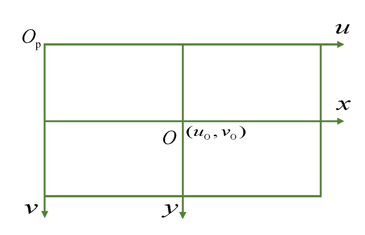
As shown in Figure 8, the image pixel coordinate system is a coordinate system that considers the upper left corner of the image as the origin. (u0, v0) represents the coordinates of the origin of the image physical coordinate system in the image pixel coordinate system.
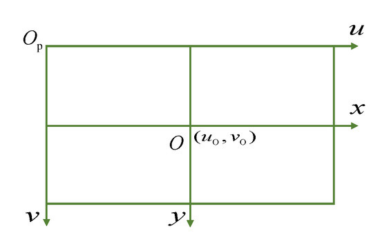
Figure 8.
The relationship between image pixel coordinate system and image physical coordinate system.
The image pixel coordinate system is transformed into an image physical coordinate system by using the following expression:
where, (u, v) represents the coordinates of the target point in the pixel coordinate system, (u0, v0) represents the coordinates of the origin of the image coordinate system in the pixel coordinate system, and dx and dy are the physical dimensions of a single pixel, respectively.
According to the principle of obtaining the 3D coordinates of the target by using binocular stereo vision, the transformation relationship from the physical coordinate system of the image to the camera coordinate system can be obtained from (1) as follows:
where, f is the focal length of the camera, (Xc, Yc, Zc) is the coordinate of the target point in the left camera coordinate system, and (x, y) is the coordinate of the target point in the image coordinate system.
Please note that both the world coordinate system and the camera coordinate system are 3D coordinate systems. The transformation between the 3D coordinate systems can be performed based on rotation and translation. Therefore, the transformation between the world coordinate system and the camera coordinate system is realized based on the following expression:
where, R3×3 is the rotation matrix of the camera coordinate system relative to the world coordinate system, T3×1 is the translation matrix of the camera coordinate system relative to the world coordinate system, (Xc, Yc, Zc) represents the coordinates of the target point in the left camera coordinate system, and (Xw, Yw, Zw) represents the target point in the world coordinate system.
Formulas (5)–(7) can be used simultaneously to transform the world coordinate system into the pixel coordinate system:
where, and .
The purpose of camera calibration is to obtain the unknown parameters of (8). Among these parameters, fx, fy, u0, and v0 are the internal parameters of the camera. Therefore, the matrix where these parameters are located is called the internal parameter matrix. The matrix composed of the rotation matrix R3×3 and the translation vector T3×1 is called the external parameter matrix.
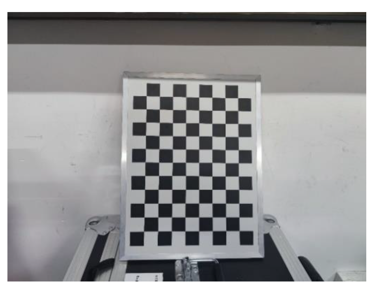
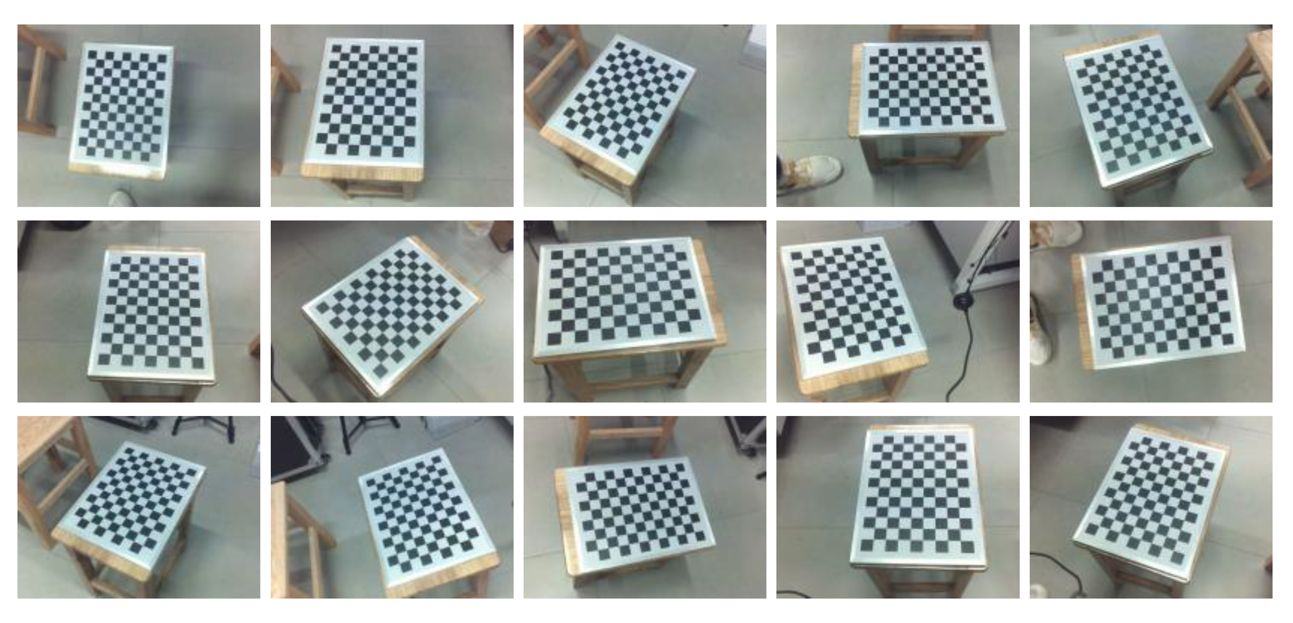
The camera calibration experiment performed in this work uses MATLAB 2017b. The calibration board used in the camera calibration experiment is a checkerboard with a grid side length of 25 mm, as shown in Figure 9.
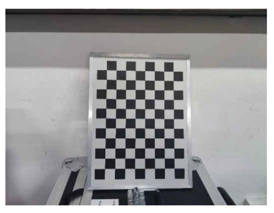
Figure 9.
The board used for camera calibration.
In this work, the method proposed by Zhang Zhengyou et al. [40] is used to perform the camera celebration. This method calibrates the camera by detecting the corners of the checkerboard. It is noteworthy that this calibration method has low requirements in terms of equipment, and only needs to print a checkerboard, thus simplifying the calibration process and guaranteeing the accuracy of the calibration.
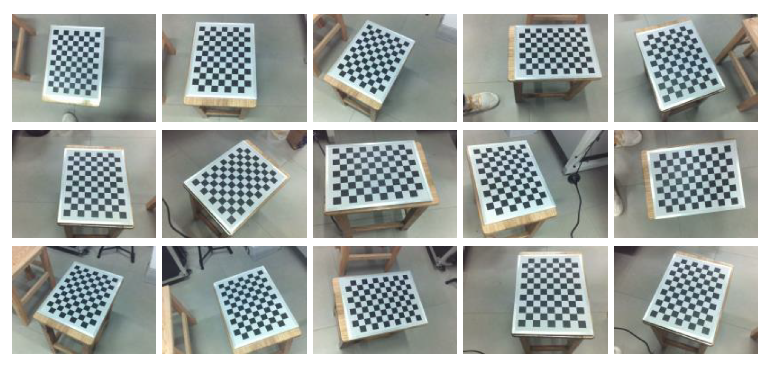
The images of the calibration board acquired by the binocular camera are shown in Figure 10 and Figure 11. The camera calibration results are shown in Table 1.
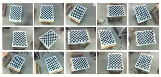
Figure 10.
The images of the calibration board acquired by the left camera.
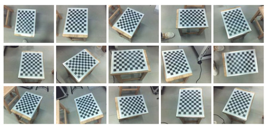
Figure 11.
The images of the calibration board acquired by the right camera.

Table 1.
The calibration results of the cameras.
4.3. Distortion Correction and Stereo Correction
The camera projects the objects on the imaging plane according to the projection principle. During this process, the difference between the manufacturing accuracy and the assembly accuracy of the lens leads to distortions in the image, which in turn affect the detection and recognition results. Therefore, it is necessary to remove the distortions from the image. The lens distortion can be divided into radial distortion and tangential distortion. Please note that these distortions need to be corrected separately.
The radial distortion is caused by the light rays being bent farther from the center of the lens as compared to near the center. The direction of the distortion is along the radius of the lens. The radial distortion model is established as shown in (9). The tangential distortion is caused when the lens is not parallel to the imaging plane of the camera. The model of the tangential distortion is shown in (10).
where, (x0, y0) denotes the original position of the distorted point on the image plane, (x, y) is the new position after the distortion is corrected, is the distance from the new position to the center of the lens, k1, k2 and k3 are the radial distortion parameters, and p1 and p2 are the tangential distortion parameters.
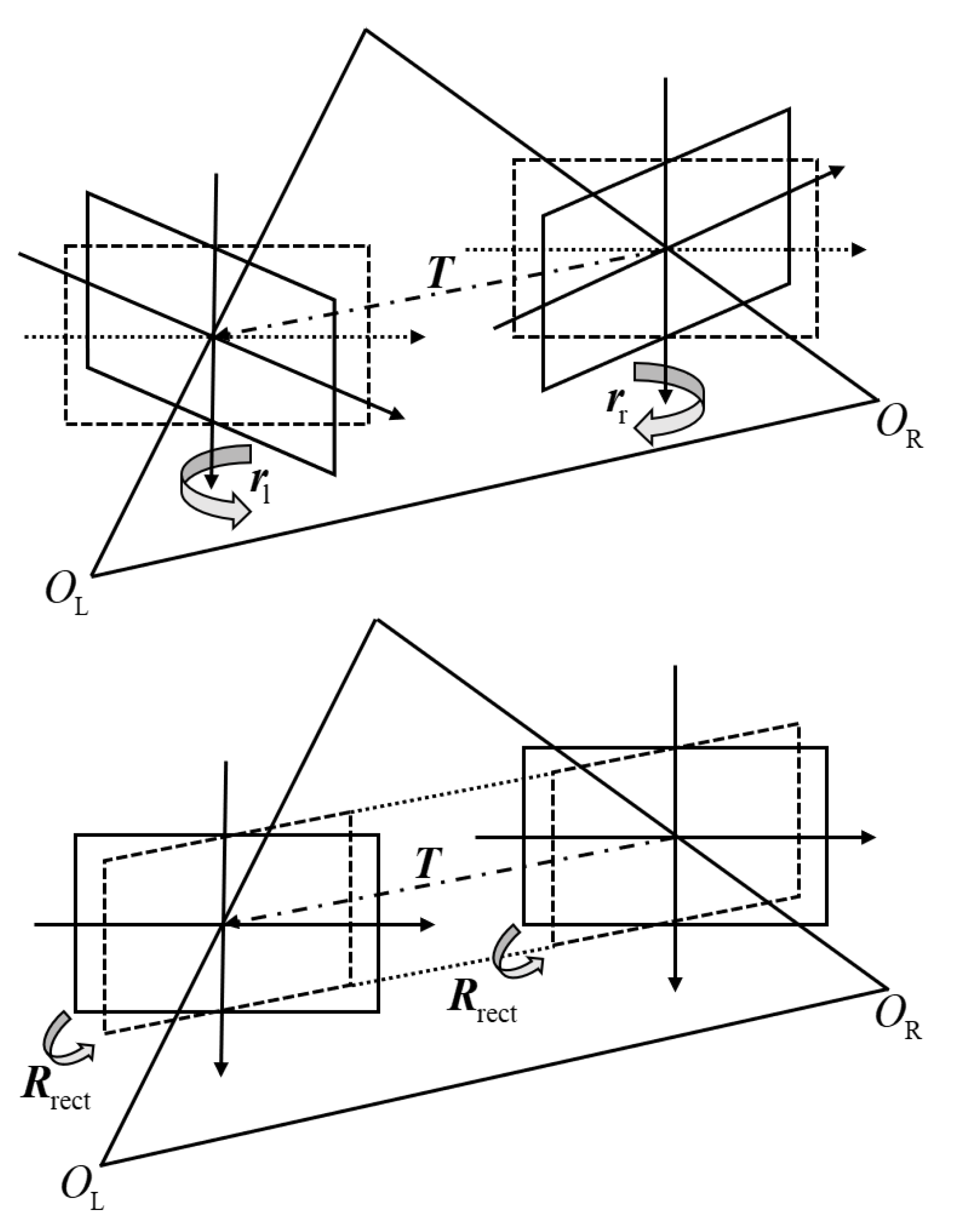
In an ideal binocular stereo vision system, the left and right camera imaging planes are coplanar, and row aligned. However, in practice, the two planes are deviated. The purpose of the stereo correction is to correct this deviation. The stereo correction process is shown in Figure 12.

Figure 12.
The process of stereoscopic correction.
The rotation matrix R3×3 and translation vector T3×1 obtained during the process of camera calibration represent the transformation required to convert the right camera coordinate system to the left camera coordinate system. In order to minimize the image reprojection distortion, we rotate the imaging plane of the left and right cameras by half R3×3. The rotation matrices of the left and right cameras are represented by rl and rr, respectively. The relationship between rl and rr is mathematically expressed as:
After the first step of rotation transformation, the imaging planes of the left and right cameras are already coplanar (parallel), but there is still no row alignment. In order to achieve row alignment of the left and right images, a new rotation matrix Rrect is constructed as:
T in Figure 12 is obtained by the camera calibration and represents the translation vector from the origin of the right camera coordinate system to the origin of the left camera coordinate system, i.e., the origins of the two coordinate systems have achieved row alignment in the direction of the vector T. Therefore, the rotation matrix Rrect is constructed according to the vector T.
The second vector e2 is orthogonal to e1, so e2 can be obtained by computing the cross product of the unit vector in the direction of the main optical axis and e1. After normalization, e2 is expressed as follows:
The third vector e3 is orthogonal to both e1 and e2.
After combining the two processes of stereo correction, the stereo correction rotation matrix of the left and right cameras is obtained by using the following expression:
After correcting the distortion and performing stereo correction, the reprojection matrix of the pixel coordinate system and the world coordinate system is obtained as follows:
where, cx and cy represent the x and y axis coordinates of the main point of the corrected left camera image, respectively, f is the focal length of the camera, and b is the baseline length.
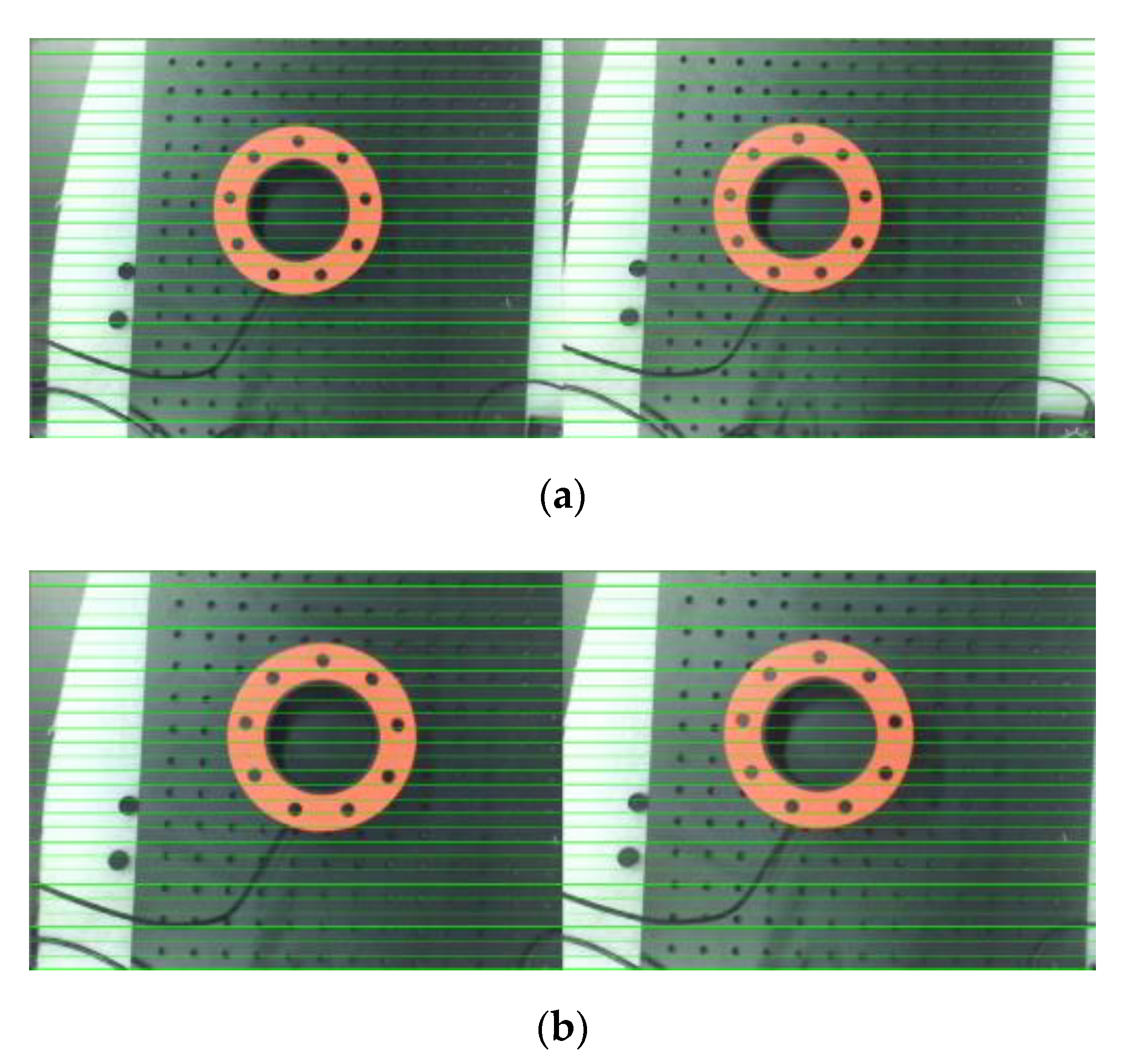
Figure 13 presents the effect of stereo correction. The row alignment is achieved in the left and right images after rectification, but the cropping operation after rectification causes the loss of partial image content. Table 2 shows the camera parameters after correction.
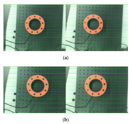
Figure 13.
The resulting images after stereoscopic correction: (a) the binocular image before correction; and (b) the binocular image after correction.
Table 2.
The corrected results of camera parameters.
4.4. Stereo Matching
The stereo matching is a key link in binocular stereo vision. The purpose of stereo matching is to match the corresponding pixels in two or more viewpoints and calculate the disparity. The disparity of the pixel point is estimated by establishing and minimizing an energy cost function. The semi-global block matching (SGBM) algorithm is a stereo matching algorithm based on the semi-global matching (SGM) [41] algorithm. As compared with the traditional global matching and local matching algorithms, the SGBM is a more balanced algorithm with a higher accuracy and computational speed. The stereo matching comprises four steps, including cost computation, cost aggregation, disparity computation, and post processing.
The SGBM algorithm combines SAD [42,43] and BT [44] algorithms for computing the matching cost, thus increasing the robustness of the algorithm. The cost of BT algorithm is mainly composed of two parts, namely the cost associated with the image processing based on the Sobelx operator and the cost associated with the original image. The edge information in the vertical direction of the image convolved by the Sobelx operator is more obvious. The matching of the edge area can be optimized by calculating the BT cost after convolving the image with the Sobelx operator. Please note that directly calculating the BT cost of the original image preserves the overall information of the image. Combining the two BT costs enhances the matching effect at the edges and the details of an image, while retaining a large amount of original image information. When the two aforementioned types of BT costs are added and combined, a SAD block calculation is performed, i.e., the cost value of each pixel is replaced by the sum of the cost values in the neighborhood. The following mathematical expression is obtained by combining the two aforementioned processes:
where, p and q denote the pixels of the left view of the camera, Np represents the neighborhood of p, (u, v) represents the coordinates of the pixels in the left camera image, Il and Ir represent the gray values of the left and right camera image pixels, respectively, and represent the gray values on the sub-pixel points of the left and right camera images, respectively, and d represents the disparity.
In the aforementioned process, for every pixel block in the left image, the matching window in the right image moves within the specified retrieval range, which means that the value of d changes within a certain limit. The costs corresponding to different values of d are recorded for cost aggregation. The energy cost function of cost aggregation is shown in (20). The goal of stereo matching is to minimize this energy cost function.
where, p and q represent the pixel point, Np represents the neighborhood of p, Dp and Dq represent the disparity values of p and q, respectively, the value of the T […] function is 1, when the conditions in the parentheses are satisfied, and zero otherwise, P1 and P2 represent the penalty coefficients, and P1 < P2. Please note that the smaller coefficients enable the algorithm to adapt the situations where the parallax change is small, such as the pixels on an inclined plane and a continuous surface. On the other hand, the larger penalty coefficients enable the algorithm to adapt the situations where the parallax changes significantly, such as the situation where the pixel is at the intersection of the edge.
In order to efficiently find the minimum value of the energy function, the SGBM algorithm uses the dynamic programming to optimize the cost aggregation. Considering a single pixel p, the cost along the path r is computed as follows:
where, the second term compares the matching cost of points on the path to p under different parallaxes and combines the penalty coefficients P1 and P2 for selecting the minimum cost. This enables to avoid the global cost aggregation operation and greatly reduces the amount of operation.
After cost calculation, the disparity value associated with the smallest matching cost of each pixel is selected based on the winner takes all (WTA) principle.
The SGBM algorithm obtains the disparity map after completing the above process. In order to make the disparity more accurate, post-processing is required, which mainly includes a uniqueness check, sub-pixel interpolation, and left-right check. Please note that the uniqueness check is used to eliminate the erroneous disparity values to avoid the local optima. The sub-pixel interpolation makes parallax smoother, and the left-right check is used to address the matching errors caused by occlusion. After finishing post-processing, the final disparity map is obtained. Figure 14 presents a comparison diagram of the disparity map and the original image.
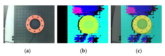
Figure 14.
The disparity image of a pipe joint: (a) original image; (b) disparity map; and (c) superimposed map.
4.5. Plane Fitting of Petroleum Pipeline Interface
After successfully obtaining the petroleum pipeline interface’s edge contour and disparity map, the disparity values of the corresponding points are obtained based on the pixel coordinates of the contour. Afterwards, a set of 3D points is obtained by using (4). Since the pipe has depth information, the 3D coordinates of the interface’s center, which are directly obtained from the disparity map, have a gap with the interface’s plane. In order to correct this gap, it is necessary to fit the plane of the petroleum pipeline interface.
The random sample consensus (RANSAC) algorithm has the ability to estimate the optimal model from a set of datasets containing abnormal data. The RANSAC algorithm extracts a small number of data samples from a given dataset and obtains a parameterized model that satisfies these samples. A fault tolerance range is usually set during the verification process. When a data sample deviates from the established model within this fault tolerance range, it can be considered that this data sample conforms to the model. The RANSAC algorithm divides the data points into inliers and outliers. The inliers refer to the data samples that can adapt to a given parameterized model. On the other hand, the outliers refer to the data samples that are unable to adapt to the model. The execution process of the RANSAC algorithm is an iterative process. When a better model is obtained, the model parameters are updated. A threshold can be set for RANSAC for reducing the number of computations. When the proportion of the inliers reaches the threshold, the iteration can be terminated early.
The model to be fitted in this work is a space plane model. The general mathematical expression for a space plane is:
The normal vector of this plane is .
Three non-collinear points define a plane. It is only necessary to select three non-collinear points from the 3D point set to complete the calculation of the parameters of the space plane expression. Assuming that the three non-collinear points are selected from the 3D points set P1, P2, and P3, two vectors and with the same starting point can be obtained from the coordinates of the three points. The normal vector of the plane equation where three points are located can be obtained by computing the cross product of these two vectors as follows:
The parameter D can be obtained by substituting any one of the three points in (15).
After obtaining the space plane equation, the accuracy of the model is verified. We calculate the distance from each point to the plane. If the distance between the point and the plane is less than the preset fault tolerance range, the point is accepted as an inlier, otherwise it is marked as an outlier. Then, we find and record the proportion of the number of inliers. The aforementioned process is repeated if the new model has a larger proportion of inliers. This indicates that the new model is a better model for a sample, and the parameters of the spatial plane equation are updated. The iterative process is stopped, and the parameters of the best model are recorded when the iteration reaches the upper limit set for the number of iterations, or the proportion of inliers reaches the set threshold.
The pixel coordinates of the center of petroleum pipeline interface obtained during the identification stage are (ucenter, vcenter). The corrected camera parameters are obtained from Table 2. The physical coordinates of the center image of the petroleum pipeline interface are (xcenter, ycenter). The relationship between (xcenter, ycenter) and (ucenter, vcenter) is expressed as follows:
It is evident from (4) that the coordinates of the petroleum pipeline interface’s center between the camera physical coordinate system and the world coordinate system are proportional to each other. The relationship between these coordinates is expressed as:
where, (Xcenter, Ycenter, Zcenter) are the world coordinate system’s coordinates of the center of the petroleum pipeline interface, (xcenter, ycenter) are the image physical coordinate system’s coordinates of the petroleum pipeline interface center, f is the focal length of the left camera and α is the proportionality coefficient.
The coordinates of the center of petroleum pipeline interface in the camera coordinate system satisfy the given optimal model. Therefore, the coefficient α can be obtained by substituting the coordinates into the plane equation as:
Finally, by substituting α in (25), the world coordinate system coordinates of the petroleum pipeline interface’s center are obtained.
Figure 15 shows the fitting plane when the lens is facing the petroleum pipeline interface. It is evident from the image that the abnormal points do not interfere with the final model as the RANSAC plane fitting algorithm is based on the valid data samples, thus making this method more robust.
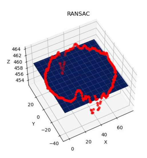
Figure 15.
The fitting plane diagram of a pipeline interface.
5. Experimental Design and Analysis
The camera used in the experiment is a fixed baseline binocular camera. The parameters of this camera are shown in Table 3. The camera is connected with the computer through a USB3.0 data cable. The proposed algorithm is implemented in C++ and runs in the VS2017 environment configured with OpenCV. In order to comprehensively verify the accuracy of the binocular stereo vision pose detection system, this work verifies the accuracy of distance measurement and angle measurement.
Table 3.
The parameters of the binocular camera.
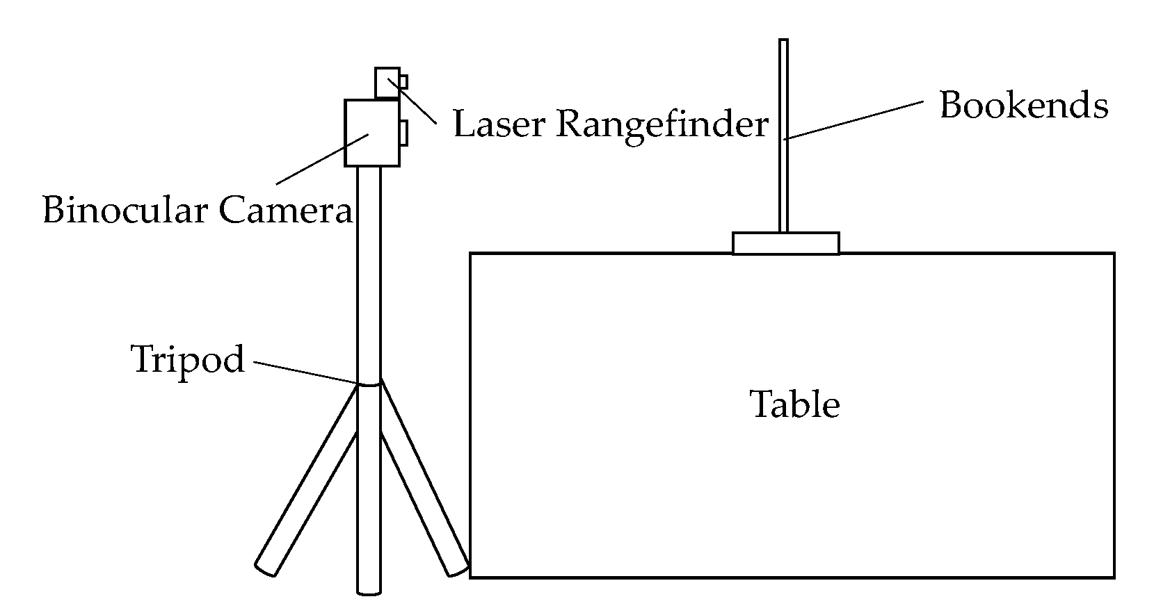
During the verification experiment performed for estimating the accuracy of measuring distance, the binocular camera is placed on a tripod, and the bookend is placed in front of the camera, as shown in Figure 16. The acquired images are input into the program for processing. Then, we compare the resulting depth values computed by the proposed method with the values of the distance obtained from the lens to the bookend measured by the laser rangefinder. In order to improve the reliability of the experimental results, this work considers 10 points from the bookend in each picture and obtains the average value of the depth values for these 10 points and uses it as the distance from the camera to the bookend. According to the binocular stereo vision ranging theory, the ranging accuracy is only influenced by the accuracy of the parallax. Therefore, the measurement accuracy of the depth also reflects the measurement accuracy of the horizontal and vertical directions. Therefore, it can be considered that the measurement accuracy of the depth represents the overall measurement accuracy of the system. The final experimental results are shown in Table 4. As compared with the actual measured distance, the maximum error of the distance value calculated by the proposed method is very low, i.e., at centimeter level, and the relative error does not exceed 1%. This error is completely acceptable for large industrial equipment. Therefore, it is feasible to apply the binocular stereo vision to the intelligent docking of the manipulator arm.
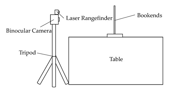
Figure 16.
The accuracy of measured distance based on the proposed method.
Table 4.
The distance between the measurement results.
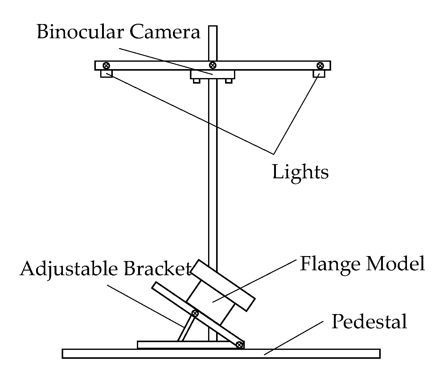
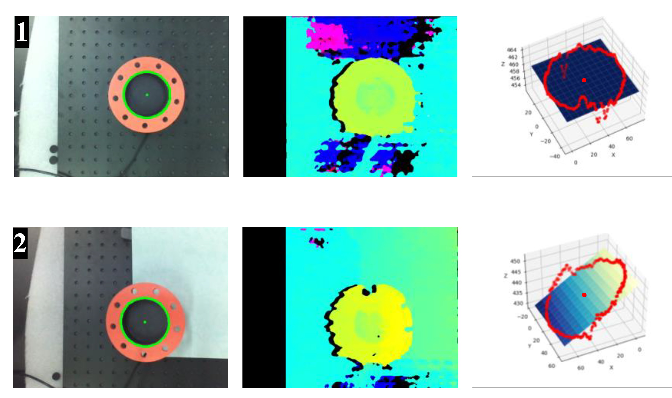
The experimental platform of the angle accuracy verification is shown in Figure 17. We identify the 3D printed flange model and place it on a bracket whose inclination angle can be adjusted. We adjust the bracket at different angles and capture the images of the model and use them as the input of the proposed method. Figure 18 shows the experimental results of the pipeline interface with different inclination angles. The inclination angle of the petroleum pipeline interface plane obtained by the proposed method is compared with the inclination angle measured by the level gauge. The experimental results are shown in Table 5. The absolute error of the angle measurement is within 1 degree. Although the accuracy of the stereo vision measurement meets the requirements of docking, please note that there are holes and dark parts in the disparity map, which are caused by large areas of weak texture and uneven illumination of the left and right cameras. This effect is limited in the edge region. However, it can be seen from the fitted plan that the smoothness of the 3D contour of the petroleum pipeline interface increases with an increase in the angle. This is because the gray values of the surface of the petroleum pipeline interface have obvious distribution as the angle increases. This greatly reduces the probability of mismatching in the stereo matching stage. Therefore, enhancing the matching accuracy is the only way for the system to be suitable for practical applications.

Figure 17.
The schematic diagram of measurement angle accuracy verification experiment.

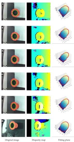
Figure 18.
The experimental results of the pipeline interface with different inclination angles: 1. 0.00°; 2. 14.02°; 3. 21.88°; 4. 30.00°; 5. 35.21°; 6. 38.20°; 7. 41.31°; and 8. 45.00°.
Table 5.
The angle measurement results.
6. Conclusions
- (1)
- This work extracts the area of the petroleum pipeline interface from the image based on color space conversion and threshold setting. This work uses the findContours function available in OpenCV to extract the contour of the petroleum pipeline interface. The extracted contours are then filtered to obtain the inner contour of the target interface. Finally, the pixel coordinates of the interface’s center are obtained by using the Hu moment.
- (2)
- This work uses MATLAB to calibrate the camera and uses the calibration parameters for image correction. The corrected left and right images are stereo matched based on the SGBM algorithm, and the disparity map based on the left camera attempt is obtained. Then, the 3D coordinates of each pixel are obtained from the disparity map according to the epipolar geometry.
- (3)
- This work uses the point cloud of the petroleum pipeline interface to fit the space plane based on the RANSAC algorithm and uses the normal vector of the fitted plane to calculate the inclination angle of the interface. Based on the relationship between the corresponding coordinates of the pixel points, the 3D coordinates of the interface’s center are obtained after combining the fitting plane equations. Finally, the pose judgment of the petroleum pipeline interface is realized.
- (4)
- This work compares the calculated depth information with the actual depth information measured by using the laser rangefinder. In addition, this work also compares the calculated inclination angle with the angle measured by using the horizontal measuring instrument. The error of the measurement distance of the whole system is very small, i.e., of the millimeter level. The measurement error in the inclination angle is less than one degree, which is acceptable for large-scale machinery. The aforementioned experiments prove that it is reasonable and feasible to use the binocular stereo vision method to judge the pose of the petroleum pipeline interface and use this information for subsequent control. As compared with the methods based on Lidar sensor and special markers, the methods based on machine vision are more flexible. As the error in the measured distance increases with an increase in the distance, it is best to control the manipulator arm iteratively and approach the target step by step.
- (5)
- The binocular stereo vision may produce large matching errors in the regions with uneven illumination and weak textures. Since the edge contour area has obvious gradient information, this effect is relatively limited. However, please note that the point cloud of the contour of the petroleum pipeline interface fluctuates significantly in a small range, when the inclination angle is 0. The violent fluctuation may lead to plane fitting errors. Therefore, improving the stability of stereo matching when the plane is parallel to the camera is a direction for future research.
Author Contributions
Conceptualization, W.F. and Z.L.; methodology, Z.L.; software, Z.L.; validation, J.M. and B.L.; formal analysis, S.Y.; investigation, X.Z.; resources, J.X.; data curation, Z.L.; writing—original draft preparation, W.F. and Z.L.; writing—review and editing, W.F., Z.L. and J.M.; visualization, Z.L.; supervision, W.F. and S.Y.; project administration, W.F. and J.X.; funding acquisition, W.F. and J.X. All authors have read and agreed to the published version of the manuscript.
Funding
This research was funded by Dinghai District School-site Cooperation Project (2019C3105) and Oil Transfer Arm Automatic Docking Technology Research and Development Project between Shanghai Eminent Enterprise Development Co., Ltd. and Zhejiang Ocean University.
Informed Consent Statement
Not applicable.
Data Availability Statement
All data used to support the findings of this study are included within the article.
Acknowledgments
The authors gratefully acknowledge the support provided by Shanghai Eminent Enterprise Development Co., Ltd. and Zhejiang Ocean University.
Conflicts of Interest
The authors declare no conflict of interest.
References
- Che, K.; Lu, D.; Guo, J.; Chen, Y.; Peng, G.; Xu, L. Noncontact Clearance Measurement Research Based on Machine Vision. In International Workshop of Advanced Manufacturing and Automation; Springer: Singapore, 2022. [Google Scholar]
- Gu, P.; Zhu, C.; Yu, Y.; Liu, D.; Wu, Y. Evaluation and prediction of drilling wear based on machine vision. Int. J. Adv. Manuf. Technol. 2021, 114, 2055–2074. [Google Scholar] [CrossRef]
- Millara, L.F.; Usamentiaga, R.; Daniel, F.G. Calibrating a profile measurement system for dimensional inspection in rail rolling mills. Mach. Vis. Appl. 2021, 32, 17. [Google Scholar] [CrossRef]
- Li, Y.; Li, J.; Yao, Q.; Zhou, W.; Nie, J. Research on Predictive Control Algorithm of Vehicle Turning Path Based on Monocular Vision. Processes 2022, 10, 417. [Google Scholar] [CrossRef]
- Abhilash, P.M.; Chakradhar, D. Machine-vision-based electrode wear analysis for closed loop wire edm process control. Adv. Manuf. 2022, 10, 131–142. [Google Scholar] [CrossRef]
- Lin, Q.; Zhou, J.; Ma, Q. Detection of the fluff fabric surface quality based on machine vision. J. Text. Inst. 2021, 8, 1666–1676. [Google Scholar] [CrossRef]
- Ropelewska, E.; Wrzodak, A.; Sabanci, K.; Aslan, M.F. Effect of lacto-fermentation and freeze-drying on the quality of beetroot evaluated using machine vision and sensory analysis. Eur. Food Res. Technol. 2021, 248, 153–161. [Google Scholar] [CrossRef]
- Nawar, A.; Sabuz, N.K.; Siddiquee, S.; Rabbani, M.; Majumder, A. Skin Disease Recognition: A Machine Vision Based Approach. In Proceedings of the 2021 7th International Conference on Advanced Computing and Communication Systems (ICACCS), Coimbatore, India, 19–20 March 2021. [Google Scholar]
- Sung, H.J.; Park, M.K.; Choi, J.W. Automatic grader for flatfishes using machine vision. Int. J. Control Autom. Syst. 2020, 18, 3073–3082. [Google Scholar] [CrossRef]
- Keenan, S.J.; Diamond, J.; Mccluggage, W.G.; Bharucha, H.; Hamilton, P.W. An automated machine vision system for the histological grading of cervical intraepithelial neoplasia (cin). J. Pathol. 2015, 192, 351–362. [Google Scholar] [CrossRef]
- Liu, G.; Zhang, R.; Wang, Y.; Man, R. Road Scene Recognition of Forklift AGV Equipment Based on Deep Learning. Processes 2021, 9, 1955. [Google Scholar] [CrossRef]
- Yang, H.; Jiang, Y.; Deng, F.; Mu, Y.; Zhong, Y.; Jiao, D. Detection of Bubble Defects on Tire Surface Based on Line Laser and Machine Vision. Processes 2022, 10, 255. [Google Scholar] [CrossRef]
- Lin, C.-S.; Pan, Y.-C.; Kuo, Y.-X.; Chen, C.-K.; Tien, C.-L. A Study of Automatic Judgment of Food Color and Cooking Conditions with Artificial Intelligence Technology. Processes 2021, 9, 1128. [Google Scholar] [CrossRef]
- Im, D.; Jeong, J. R-CNN-Based Large-Scale Object-Defect Inspection System for Laser Cutting in the Automotive Industry. Processes 2021, 9, 2043. [Google Scholar] [CrossRef]
- Tuan, N.M.; Hau, Q.V.; Chin, S.; Park, S. In-situ concrete slump test incorporating deep learning and stereo vision. Autom. Constr. 2021, 121, 103432. [Google Scholar] [CrossRef]
- Afzaal, H. Estimation of soil surface roughness using stereo vision approach. Sensors 2021, 21, 4386. [Google Scholar]
- Kardovskyi, Y.; Moon, S. Artificial intelligence quality inspection of steel bars installation by integrating mask r-cnn and stereo vision. Autom. Constr. 2021, 130, 103850. [Google Scholar] [CrossRef]
- Gunatilake, A.; Piyathilaka, L.; Tran, A.; Viswanathan, V.; Kodagoda, S. Stereo vision combined with laser profiling for mapping of pipeline internal defects. IEEE Sens. J. 2020, 21, 11926–11934. [Google Scholar] [CrossRef]
- Pozo, F.; Vidal, Y. Wind turbine fault detection through principal component analysis and statistical hypothesis testing. Energies 2016, 9, 3. [Google Scholar] [CrossRef]
- Wang, J.; Gao, R.; Yan, R. Integration of EEMD and ICA for wind turbine gearbox diagnosis. Wind Energy 2014, 7, 757–773. [Google Scholar] [CrossRef]
- Yampikulsakul, N.; Byon, E.; Huang, S.; Sheng, S.; You, M. Condition monitoring of wind power system with nonparametric regression analysis. IEEE Trans. Energy Convers. 2014, 29, 288–299. [Google Scholar]
- Santos, P.; Villa, L.; Reñones, A.; Bustillo, A.; Maudes, J. An SVM-based solution for fault detection in wind turbines. Sensors 2015, 15, 5627–5648. [Google Scholar] [CrossRef]
- Gao, Z.; Liu, X. An Overview on Fault Diagnosis, Prognosis and Resilient Control for Wind Turbine Systems. Processes 2021, 9, 300. [Google Scholar] [CrossRef]
- Li, Y.; Li, W.; Darwish, W.; Tang, S.; Hu, Y.; Chen, W. Improving Plane Fitting Accuracy with Rigorous Error Models of Structured Light-Based RGB-D Sensors. Remote Sens. 2020, 12, 320. [Google Scholar] [CrossRef] [Green Version]
- Hamzah, R.A.; Ibrahim, H. Improvement of disparity map refinement stage using adaptive least square plane fitting technique. Electron. Lett. 2020, 56, 918–920. [Google Scholar] [CrossRef]
- Yu, C.; Ji, F.; Xue, J. Cutting plane based cylinder fitting method with incomplete point cloud data for digital fringe projection. IEEE Access 2020, 8, 149385–149401. [Google Scholar] [CrossRef]
- Kermarrec, G.; Lsler, M.; Hartmann, J. Analysis of the temporal correlations of tls range observations from plane fitting residuals. ISPRS J. Photogramm. Remote Sens. 2021, 171, 119–132. [Google Scholar] [CrossRef]
- Fischler, M.A.; Bolles, R.C. Random sample consensus: A paradigm for model fitting with applications to image analysis and automated cartography. Commun. ACM 1981, 24, 381–395. [Google Scholar] [CrossRef]
- Sevgen, S.C.; Karsli, F. An improved ransac algorithm for extracting roof planes from airborne lidar data. Photogramm. Rec. 2020, 35, 40–57. [Google Scholar] [CrossRef]
- Vongbunyong, S.; Thamrongaphichartkul, K.; Worrasittichai, N.; Takutruea, A. Automatic precision docking for autonomous mobile robot in hospital logistics—case-study: Battery charging. In IOP Conference Series: Materials Science and Engineering; IOP Publishing: Ubon Ratchathani, Thailand, 2021; Volume 1137, p. 012060. [Google Scholar]
- Nigam, A.; Penate-Sanchez, A.; Agapito, L. Detect globally, label locally: Learning accurate 6-dof object pose estimation by joint segmentation and coordinate regression. IEEE Robot. Autom. Lett. 2018, 3, 3960–3967. [Google Scholar] [CrossRef]
- Alqudah, A.M.; Alqudah, A. Improving machine learning recognition of colorectal cancer using 3d glcm applied to different color spaces. Multimed. Tools Appl. 2022, 81, 10839–10860. [Google Scholar] [CrossRef]
- Schwarz, M.W.; Cowan, W.B.; Beatty, J.C. An experimental comparison of rgb, yiq, lab, hsv, and opponent colour models. ACM Trans. Graph. 1987, 6, 123–158. [Google Scholar] [CrossRef]
- Amita, N.; Vidhyacharan, B.; Arvind, D. Contrast based image enhancement algorithm using grayscale and colour space. IET Signal Process. 2018, 12, 514–521. [Google Scholar]
- Laganiere, R. Opencv 2 Computer Vision Application Programming Cookbook: Over 50 Recipes to Master This Library of Programming Functions for Real-Time Computer Vision; Packt Publishing: Birmingham, UK, 2011. [Google Scholar]
- Kubrikov, M.V.; Saramud, M.V.; Karaseva, M.V. Method for the optimal positioning of the cutter at the honeycomb block cutting applying computer vision. IEEE Access 2021, 9, 15548–15560. [Google Scholar] [CrossRef]
- Itoh, M.; Chua, L.O. Imitation of visual illusions via opencv and cnn. Int. J. Bifurc. Chaos 2008, 18, 3551–3609. [Google Scholar] [CrossRef]
- Uni, J.; Hirota, K.; Rosin, P.L. A hu moment invariant as a shape circularity measure. Pattern Recognit. 2010, 43, 47–57. [Google Scholar]
- Žunić, D.; Žunić, J. Shape ellipticity from hu moment invariants. Appl. Math. Comput. 2014, 226, 406–414. [Google Scholar] [CrossRef]
- Zhang, Z. A flexible new technique for camera calibration. IEEE Trans. Pattern Anal. Mach. Intell. 2000, 22, 1330–1334. [Google Scholar] [CrossRef]
- Hirschmüller, H. Stereo processing by semiglobal matching and mutual information. IEEE Trans. Pattern Anal. Mach. Intell. 2007, 30, 328–341. [Google Scholar] [CrossRef]
- Alsaade, F.; Fouda, Y.M. Template matching based on sad and pyramid. Int. J. Comput. Sci. Inf. Secur. 2012, 10, 17–20. [Google Scholar]
- Skoglund, J.; Felsberg, M. Covariance Estimation for SAD Block Matching. In Proceedings of the Image Analysis, Proceedings of the 15th Scandinavian Conference, SCIA 2007, Aalborg, Denmark, 10–14 June 2007; Springer: Berlin/Heidelberg, Germany, 2007. [Google Scholar]
- Birchfield, S.; Tomasi, C. Depth discontinuities by pixel-to-pixel stereo. Int. J. Comput. Vis. 1999, 35, 269–293. [Google Scholar] [CrossRef]


Publisher’s Note: MDPI stays neutral with regard to jurisdictional claims in published maps and institutional affiliations. |
© 2022 by the authors. Licensee MDPI, Basel, Switzerland. This article is an open access article distributed under the terms and conditions of the Creative Commons Attribution (CC BY) license (https://creativecommons.org/licenses/by/4.0/).