A Combined CFD-Response Surface Methodology Approach for Simulation and Optimization of Arsenic Removal in a Fixed Bed Adsorption Column

Abstract

An experimentally validated CFD model was developed for lab-scale arsenic (As) fixed-bed columns using COMSOL Multiphysics. The effects of key factors such as the adsorbent bed depth, the feed flow rate, and the initial As concentration (conc.) on the overall As removal performance were investigated. Subsequently, the CFD was combined with response surface methodology (RSM) to optimize process conditions and examine main and interaction effects of these factors on model responses, i.e., the As removal efficiency and the bed saturation time. The ANOVA results suggested that quadratic regression models were highly significant for both responses. The established regression model equations predicted the response values closer to CFD measurements. It was found that, compared with the initial As conc. and the feed flow rate, the effect of the bed depth was more significant. Moreover, both the As removal efficiency and the bed saturation time were increased reasonably with the increasing bed depth and decreased with the increasing feed flow rate and initial As conc. The optimum conditions for the As removal process were obtained as the bed height of 80 cm, the initial As concentration of 2.7 mmol/m³, and the feed flow rate of 1 L/min. The present combined CFD−RSM approach is a useful guideline in overall design and optimization of various lab-scale and industrial applications for removal of As from wastewater.

1. Introduction

Industrial wastewater and domestic contaminated water remain a major concern in Pakistan similar to the rest of developing countries [1]. In the developing world, one of the key environmental issues related to the contamination of water is the presence of heavy metals which results into toxicity [2,3]. Arsenic (As) is one of the heavy metals which is commonly found either as As(III) or As(V) forms in the groundwater [4,5,6]. The direct (drinking) or indirect (irrigation or cattle breeding purposes) consumption of As-contaminated water leads to severe health effects on human life [7]. Moreover, water pollution increases by discharging of As-contaminated wastewater in freshwater bodies [8]. Usually, the activities of sand soils and arsenoparite rocks release minerals and contaminated underground water with As. As is also transferred in traceable conc., when water is taken out through borings and tube wells. According to the standards of World Health Organization (WHO) and US Environmental Protection Agency (EPA), the safe limit of As in water is considered to be 10 ppb [9]. Groundwater reservoirs in Pakistan, especially in the province of Sindh, are highly enriched with As. Thus, the local community mainly consuming groundwater for households as well agricultural purposes has been facing several diseases. Therefore, removal of As from groundwater has become a serious issue.

Over the past two decades, development of cost-effective technologies for As removal from water systems has been a scientific interest. Compared with a number of physicochemical methods that have been employed, i.e., adsorption [10,11], coagulation, reverse osmosis [12], and lime softening and precipitation, adsorption is popular and most efficient [13,14] among the said technologies which are used extensively due to simplicity in operation, cost-effectiveness, environmental friendliness, and presence of numerous adsorbents (naturally and synthetically) [15].

As adsorption efficiency depends upon several design parameters, e.g., the nature of adsorbents, the bed depth, the initial conc. of As, and the feed flow rate. To develop a relationship between multiple factors, the As removal efficiency is a very time-consuming and complicated approach which is not possible to achieve through one-time-one-factor (OTOF) analysis [16]. Moreover, the OTOF analysis does not provide adequate information about the interaction of different key factors. For this purpose, the design-of-experiments (DOE) method can desirably be employed which gives a sufficient understanding about the interaction between multiple factors using statistical models. In the past, several studies have been reported which used different DOE methods such as factorial design [16,17,18] and response surface methodology (RSM) [19,20,21] in combination with CFD to optimize the design of various engineering applications. RSM has been extensively used in a huge number of studies as an outstanding statistical tool for optimization [22,23,24]. It has been employed effectively for optimizing the performance of arsenic removal from aqueous solutions [25,26,27,28].

Therefore, in the initial stage of this study, As removal through fixed-bed adsorption was investigated experimentally in a lab-scale column under limited operating conditions. Subsequently, a CFD model was developed in COMSOL Multiphysics for the investigation of the As removal efficiency and the adsorbent bed saturation time. The model was validated with experimental measurements in satisfactory agreement. Finally, the validated model was combined with RSM to optimize the design of a lab-scale fixed-bed adsorption process for As removal.

2. Methodology

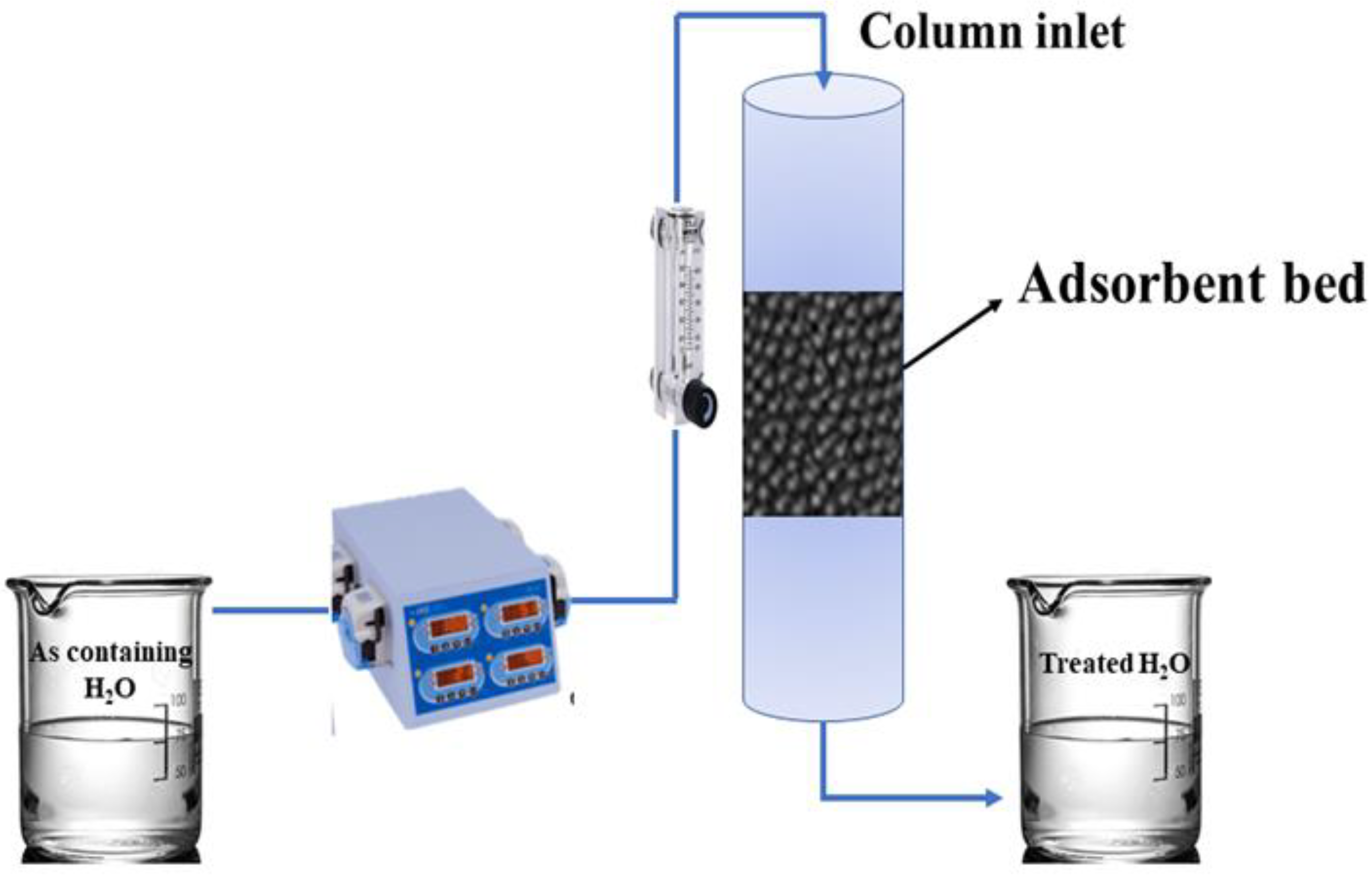
2.1. Experimental Setup and Material Selection

The experimental setup is depicted schematically in Figure 1. Experiments were performed in a cylindrical column with an inner diameter of 8 cm which consisted of a 60 cm deep adsorbent bed. A feedstock solution was introduced into the column at the top, while a clean liquid was drained out through the bottom. As already mentioned, the major objective of the study was focused on the use of a combined CFD−RSM approach. Therefore, the experiments were restricted to a limited range of the operating conditions, and their findings were used for the validation of the CFD model. Iron ore was used as an adsorbent, which was collected locally and prepared to have a desirable size using a jaw crusher (1–10 mm size; Yoshida Seisakusho Co., Ltd. Tokyo, Japan) followed by grinding in a brown crusher (<1 mm; Yoshida Seisakusho Co., Ltd. Tokyo, Japan). Particles with a required size (~600 µm) were obtained using a sieve shaker. The grinded samples were sieved using a Ro-Tap type Sieve Shaker (Heiko Seisakusho Co., Ltd. Tokyo, Japan) to obtain particles with a 600 μm size by ASTM sieves. The ore samples were washed with deionized water (Elgastat, Micromeg Deioniser) several times to remove impurities until runoff was clear and dried at 105 °C. A synthetic solution of As was prepared by the dissolution of sodium meta arsenite (AsNaO₂) (Sigma-Aldrich, St. Louis, MI, USA) in distilled water at an initial conc. of 2.7 mmol/m³. Feed flowrate conditions were set to 1 L/min, 2 L/min, and 3 L/min, which were maintained by using a peristaltic pump. All the experiments were performed under ambient temperature.

2.2. Model Development and Numerical Setting

The numerical model was developed in commercial CFD software COMSOL. The two-dimensional geometry of a column had a diameter of 8 cm. Three different heights of the bed were taken, i.e., 40, 60, and 80 cm. Figure 2 shows the developed geometry and computational grid for the simulations. The MUMPS solver was used in COMSOL. The MUMPS solver works on general systems of the form Ax = b and uses several preordering algorithms to permute the column and thereby minimize the fill-in. Relative tolerance is the convergence criteria in COMSOL, which was set at 0.001 for computations. The time steps were set to 0.1 min due to the time-dependent solution.

COMSOL uses physics-based built-in features for generating meshes, which is suitable for the selected physics. After generating the grids, the minimum orthogonal quality of the developed computational grid was calculated as 0.8364, which showed a high quality of the mesh, and the quality plays a significant role in the accuracy and stability of numerical computation [29]. In CFD, the mesh quality could be evaluated with several quality indicators among which orthogonality is one important quality parameter. Orthogonal quality was computed for cells using cell skewness and the vector from the cell centroid to each of its faces, the corresponding face area vector, and the vector from the cell centroid to the centroids of each of the adjacent cells. If the orthogonality exceeds the limits, the numerical error will be higher, which will lead to solution convergence issues. The minimum orthogonal quality for all types of cells should be more than 0.01, with an average value that is significantly higher. As the geometry is simple and less complex, the triangular mesh elements were used which could give a better solution with less consumption of time. The total size of the mesh was 927 cells. The critical mesh statistics is given in

Table 1. Statistics of the mesh.

Sr. No.	Parameter	Value
1	Sequence selected in COMSOL	Physics-controlled mesh
2	Element size feature	Extremely fine
3	Shape of elements	Triangular
4	Number of elements	927
5	Edge elements	115
6	Vertex elements	8
7	Minimum orthogonal quality	0.8364
8	Average element quality	0.974
9	Element area ratio	0.2703
10	Mesh area	0.408 m2
11	Maximum growth rate	1.619
12	Average growth rate	1.074
13	Curvature factor	0.3

.

The grid independence test is an important activity to check the optimized size of the grid by creating grids with different element sizes (density of the grid) and then simulating a few basic cases on all created grids. In this regard, three grids were created for the present research, namely finer (294 elements), extra fine (927 elements), and extremely fine (3434 elements). Three preliminary simulations were performed at a 40 cm bed depth and a 1 lit/min flow rate with varying feed concentrations, i.e., 2.7, 4.0, and 5.3 mmol/m³ (more details in

Table 2. Simulation parameters.

Sr. No	Varying Parameter	Values
1	Feed flow rate (L/min)	1
		2
		3
2	Initial arsenic concentration (mol/m3)	2.7 (200 ppb)
		4.0 (300 ppb)
		5.3 (400 ppb)
3	Bed depth (cm)	40
		60
		80

). Breakthrough curves were calculated from all simulated cases and are presented in Figure 3. From the figure, it was observed that the extra fine and extremely fine meshes gave almost similar results with a very minimum difference, whereas computations with finer meshes has a significant difference. Hence, the extra fine mesh was considered an optimized mesh and used for further simulations.

2.2.1. General Assumptions

In process simulations, the pressure drop of the liquid phase was assumed to be constant, and mixing occurring in the liquid phase was considered.

2.2.2. CFD Model Equations

In COMSOL, the “The Transport of Diluted Species (TDP)” utility was selected to model the arsenic adsorption from a porous bed of the adsorbent. This interface offers a built-in modeling environment for investigating and studying the progression of chemical species transported through convection and diffusion. Dilute species presences are assumed in this physics interface, which means that their concentrations are much smaller as compared to that of a solvent solid or fluid. The diffusion of dilute mixtures, solutes, or solutions is governed by Fick’s law, while migration of ion phenomenon is sometimes considered as an electrokinetic flow.

Mass Balance Equation

In the TDP interface, the default node models transport of chemical species through convection and diffusion and solves the conservation equation of mass for one or more chemical species attributed as i, as mathematically described by Equation (1):

$$\frac{\partial c_i}{\partial t}+\nabla . J_i+\mathbf{u}. \nabla {\mathrm{c}}_i=R_i,$$

(1)

where c_i is the specie concentration (mol/m³), R_i is the rate of reaction (mol/(m³·s)), u is the mass-averaged velocity vector (m/s), and J_i is the diffusive mass flux vector (mol/(m²·s)). Both the transport mechanisms of convection and diffusion are included in Equation (1).

The diffusive mass flux vector J_i is used for flux computation and in boundary conditions. The molecular diffusion is included in the mass transport calculated by transport of the diluted species interface. The mass flux vector J_i is calculated using Equation (2):

$$J_i=-D \nabla \mathrm{c}.$$

(2)

Adsorption Mechanism

During the traveling of species through a porous zone or medium, they typically attach to (adsorb) and detach (desorb) from the solid phase, which slows down the chemical transport through the porous medium. The species concentration in the fluid increases or decreases with adsorption or desorption, respectively. The adsorption properties vary between chemicals, so a plume containing multiple species can be separated into components [30]. The adsorption feature includes four predefined and one user-defined relationships known as isotherm models to predict the solid concentrations, c_Pi, from the concentration in the liquid phase, c_i. The most common is the Langmuir isotherm (Equation (3)), which was used in this research:

$$C_P=C_{Pmax}\frac{K_{L}c}{1+K_{L}c},$$

(3)

where K_L is the Langmuir constant and expressed in m³/mol and c_Pmax is the adsorption maximum and expressed in mol/kg. The values of K_L and c_pmax were 2122.529 m³/mol and 0.0024 mol/kg, respectively, which were estimated from previous simulation studies [31].

The time evolution of the adsorption, the solute transport to or from the solid phase, is defined by assuming that the amount of the solute adsorbed by the solid, c_P,i, is a function of the concentration in the fluid c_i. This implies that the solute concentration in the liquid and solid phases are in instant equilibrium. The adsorption term can be expanded to given by following equation:

$$\frac{\partial }{\partial t}\left(\rho c_{P,i}\right)=\rho \frac{\partial c_{P,i}}{\partial c_i}\frac{\partial c_i}{\partial t}-c_{P,i}{\rho }_s\frac{\partial {\epsilon }_p}{\partial t}=\rho K_{P,i}\frac{\partial c_i}{\partial t}\frac{\partial c_i}{\partial t}-c_{P,i}{\rho }_s\frac{\partial {\epsilon }_p}{\partial t},$$

(4)

where K_P,i is the adsorption isotherm and described as K_P,i = ∂c_P,i/∂c_i.

Convection in a Porous Medium

Convection (also called advection) describes the movement of a species, such as a pollutant, with the bulk fluid velocity. The velocity field u corresponds to a superficial volume average over a unit volume of the porous medium, including both pores and matricess. This velocity is sometimes called Darcy velocity and defined as a volume flow rate per unit cross-section of the medium. This definition makes the velocity field continuous across the boundaries between porous regions and regions with free flow. The average linear fluid velocities $u_a$ provides an estimate of the fluid velocity within the pores:

$$u=\frac{u}{{\epsilon }_P}\text{ Staurated},$$

(5)

$$u_a=\frac{u}{{\theta }_1}\text{ Unsaturated},$$

(6)

where ε_p is the porosity, θ_l is the liquid volume fraction and described as θ_l = s ε_p, and s is the saturation, a dimensionless number between 0 and 1.

2.2.3. Simulation Parameters

Numerical simulations were performed by varying feed flow rates, inlet concentrations, and bed depths. The information regarding varying parameters is described in Table 2. In the CFD simulations, an iron ore material was selected as an absorbent.

2.3. Response Surface Methodology (RSM)

In this study, RSM was used to investigate the main and combined effects of three key factors, which include the following: (A) bed depth (cm), (B) initial As concentration, and (C) feed flow rate, on the As removal efficiency (%) and the bed saturation time (min). A user-defined design (UDD) was used to develop a three-level-three-factorial design of CFD simulation runs. The standard codes, i.e., −1, 0, and 1, were taken to express the low, intermediate, and high levels of design factors, respectively. The different levels values of all the design factors are given in

Table 3. Factors and their levels for UDD.

Factors	Symbol	Levels
		Low Level (−1)	Intermediate Level (0)	High Level (1)
Bed depth (cm)	A	40	60	80
Initial As conc. (mmol/m3)	B	2.7	4.0	5.3
Feed flow rate (L/min)	C	1	2	3

.

Using a regression equation, the analysis of response was performed in Design Expert 8.0. The main effects of independent variables (design factors) are represented by A, B, and C, while the interaction effects between factors can be expressed as AB, AC, and BC.

3. Results and Discussion

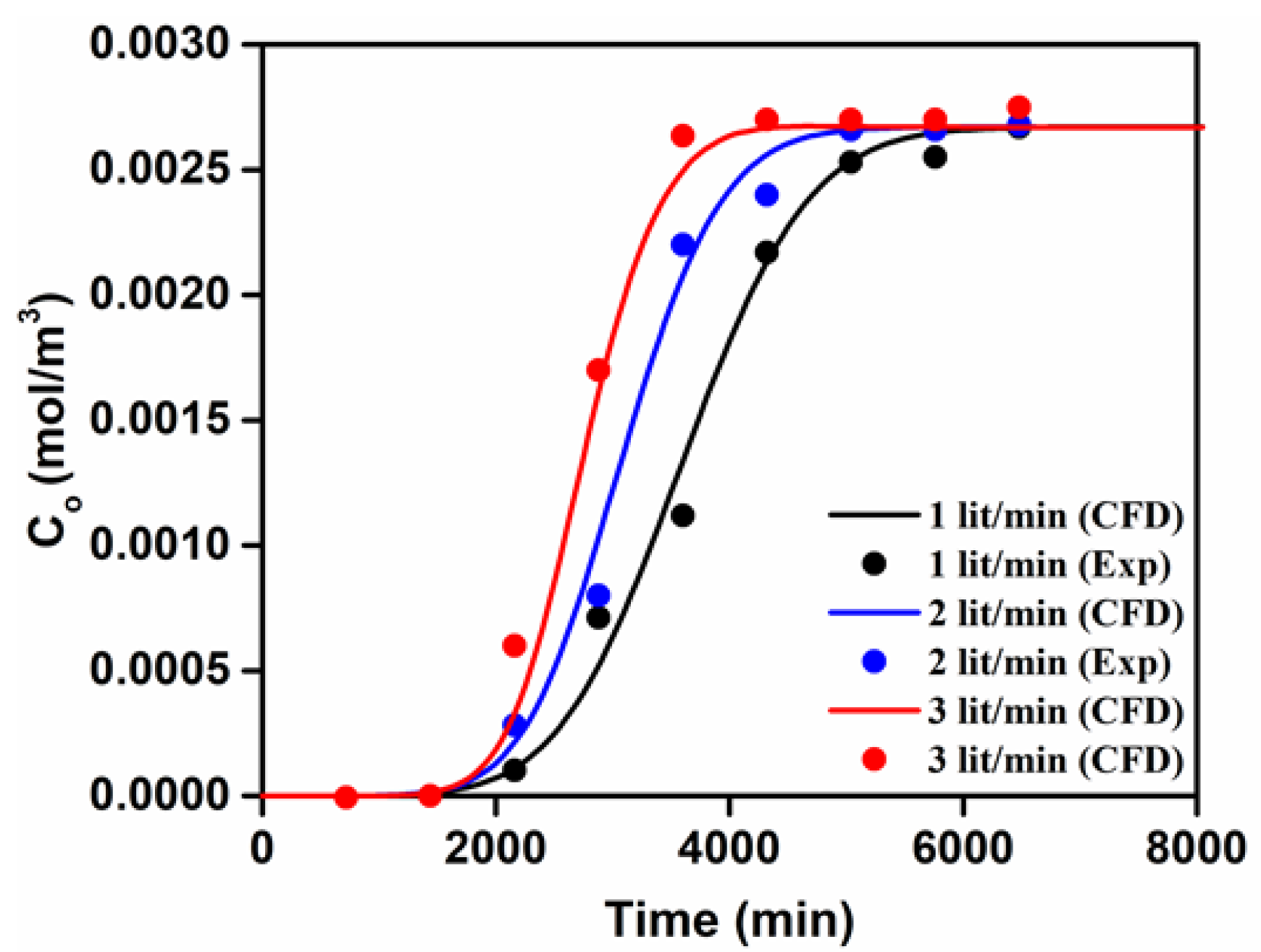
3.1. Model Validation

The CFD model was validated by comparing the CFD-predicted values of outlet concentration of As with those measured experimentally under the conditions of an adsorbent bed depth of 60 cm and varying feed flow rates of 1 L/min, 2 L/min, and 3 L/min. As depicted in Figure 4, both the findings were obtained in satisfactory agreement, suggesting the reasonable accuracy of the presently proposed CFD model to develop a deep insight into the As removal process.

3.2. CFD Results—Effects of the Bed Depth, the Feed Flow Rate, and the Initial Arsenic Concentration

In any adsorption system, the most important operating parameters are the flow rate of the feed stream, the initial conc. of impurity present, and the depth of the adsorbent bed. In the breakthrough curve, the ratio of the outlet conc. to the inlet conc. is plotted against time. Figure 5 shows the different scenarios regarding the variation of operating parameters. From Figure 5, it has been observed that increasing the feed flow rate (moving from the left to the right of plots) the bed saturation time was decreased. This could be attributed to deposition of more As on the bed in a given time and ultimately speed-up of the bed saturation. Similarly, the initial As conc. increased (going downwards in the plots), and the bed saturation time decreased under the given conditions. However, the bed depth posed an opposite effect on its saturation time, such that bed saturation time was increased with the increasing depth. It can be demonstrated that the increase in the depth of bed directly increased the mass and hence the volume of the material, which gave higher adsorption sites for As compared to a lower bed depth.

3.3. RSM Results

3.3.1. ANOVA Results and Models Regression

The results of both the responses R1 (As removal efficiency (%)) and R2 (bed saturation time (min)) are enlisted in

Table 4. Factors design matrix and responses.

Run	A: Bed Depth (cm)	B: Initial As Conc. (mol/m3)	C: Feed Flow Rate (L/min)	As Removal Efficiency (%)	Bed Saturation Time (mins)
1	−1	−1	−1	71.58	3050
2	0	1	1	62.88	2100
3	−1	−1	0	56.64	2700
4	0	−1	−1	99.56	6550
5	−1	0	0	3.55	1750
6	0	0	−1	99.37	4000
7	−1	−1	1	44.04	2500
8	1	1	1	100	3100
9	1	−1	−1	99.99	10,750
10	1	0	−1	99.99	6750
11	1	1	−1	99.99	4800
12	1	0	0	99.99	5150
13	0	−1	1	99.44	4350
14	0	−1	0	99.35	5450
15	1	1	0	99.99	3950
16	−1	1	1	0	1100
17	−1	1	0	0	1200
18	−1	1	−1	0	1350
19	−1	0	−1	13.82	1900
20	1	−1	1	99.99	7100
21	−1	0	1	0.32	1550
22	0	0	1	95.83	2900
23	1	−1	0	99.98	8550
24	0	0	0	98.53	3250
25	1	0	1	99.98	4450
26	0	1	0	91.05	2450
27	0	1	−1	97.37	2800

, which show that factors and their levels had significant effects on both the responses.

According to the analysis of variance (ANOVA) as illustrated in

Table 5. ANOVA results for response surface quadratic model responses, R1: As removal efficiency; R2: bed saturation time.

R1: As Removal Efficiency
Source	SS	df	Mean Square	F-Value	p-Value
Model	39,780.58	9	4420.06	54.81	<0.0001	Significant
A: bed depth	27,849.99	1	27,849.99	345.34	<0.0001
B: initial As concentration	2232.15	1	2232.15	27.68	<0.0001
C: feed flow rate	222.94	1	222.94	2.76	0.1147
AB	2207.48	1	2207.48	27.37	<0.0001
AC	99.28	1	99.28	1.23	0.2826
BC	1.17	1	1.17	0.0145	0.9057
A2	6971.75	1	6971.75	86.45	<0.0001
B2	195.01	1	195.01	2.42	0.1384
C2	0.8165	1	0.8165	0.0101	0.9210
Residual	1370.96	17	80.64
Cor total	41,151.55	26
R2: Bed Saturation Time
Model	1.466 × 108	9	1.629 × 107	244.33	<0.0001	Significant
A: bed Depth	7.813 × 107	1	7.813 × 107	1171.83	<0.0001
B: initial As concentration	4.402 × 107	1	4.402 × 107	660.33	<0.0001
C: feed flow rate	9.102 × 106	1	9.102 × 106	136.53	<0.0001
AB	8.250 × 106	1	8.250 × 106	123.75	<0.0001
AC	3.521 × 106	1	3.521 × 106	52.81	<0.0001
BC	1.172 × 106	1	1.172 × 106	17.58	0.0006
A2	2.963 × 105	1	2.963 × 105	4.44	0.0502
B2	2.022 × 106	1	2.022 × 106	30.33	<0.0001
C2	89,629.63	1	89,629.63	1.34	0.2623
Residual	1.133 × 106	17	66,669.39
Cor Total	1.477 × 108	26

, for R1 and R2, the model p-values were obtained as <0.0001. This implied that both models can desirably be employed to describe the statistical results and investigate the optimum conditions [32] for an As removal process. The present analysis showed that for R1 the As removal efficiency, A (bed depth), B (initial As conc.), AB (interaction of the bed depth and the initial As conc.), and A² (second-order bed depth) were taken as more significant model terms as compared to C (feed flow rate) on the basis of their p-values. For bed saturation time R2, p-values of A, B, C, AB, AC, BC, and B² suggested them as significant models’ terms. In addition to p-values, the F-values of models and their variables are also characteristic terms to describe their influential extents [33].

3.3.2. The Regression Model Equations

The regression analysis was performed to establish the fitting equations for R1 and R2 as a function of the bed depth (A), the initial As conc. (B), the feed flow rate (C), and their interaction effects, which are presented in

Table 6. Regression model equations for R1 and R2 and values of R².

Response	Regression Model	R2	Adjusted R2	Predicted R2
R1: As removal efficiency	−105.861 + 9.87085A − 63990.6B − 9.73762C + 508.093AB + 0.143817AC − 233.545BC − 0.0852188A2 + 3.20023 × 106B2 − 0.368892C2	0.9667	0.949	0.9152
R2: bed saturation time	2033.11 + 216.045A − 2.38616 × 106B − 512.523C + 31,061.9AB − 27.0833AC + 234,135 BC + 0.555556A2 + 3.25894 × 108B2 + 122.222C2	0.9923	0.9883	09764

. In each equation, the positive (+) and negative (-) signs indicate the synergistic and antagonistic effects of the model variables, respectively. R² values for both regression equations were closer to 1 which showed the models could effectively be used for the prediction of responses in terms of selected variables. Moreover, the significance of the established regression equations can be proved based on the marginal difference between adjusted R² and predicted R². According to the equations, the As removal efficiency was directly proportional to the bed depth, the interaction effect of the bed depth and the initial As conc., the interaction effect of the bed depth and the feed flow rate, the second-order bed depth, and the initial As concentration, whereas it was inversely proportional to the initial As concentration, the feed flow rate, the interaction effect of the initial concentration and the feed flow rate, and the squared feed flow rate. Similarly, the relationship between bed saturation time R2 and the model variables can be drawn from the regression equation of R2.

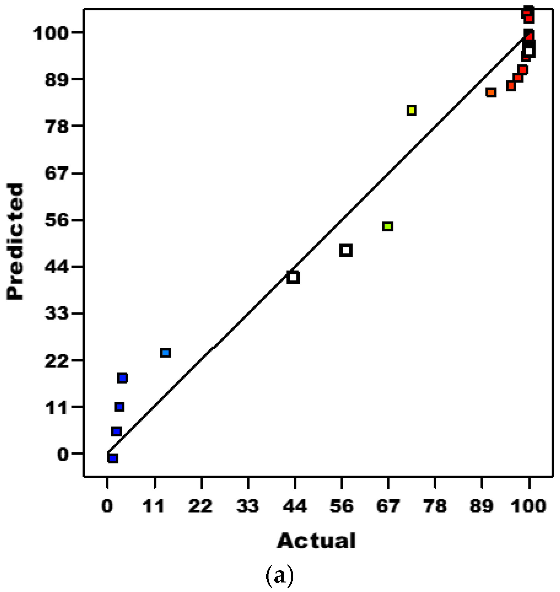
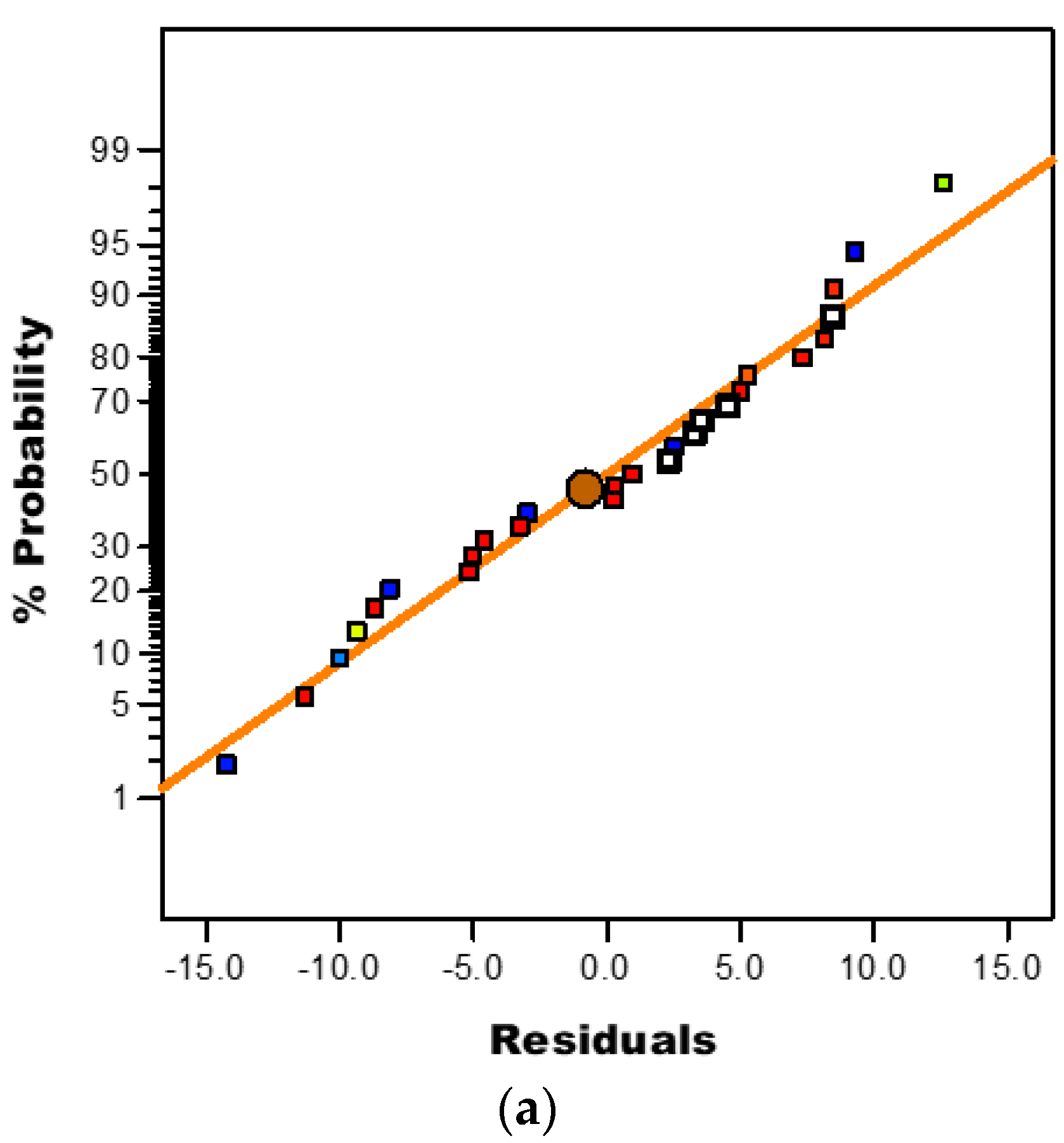
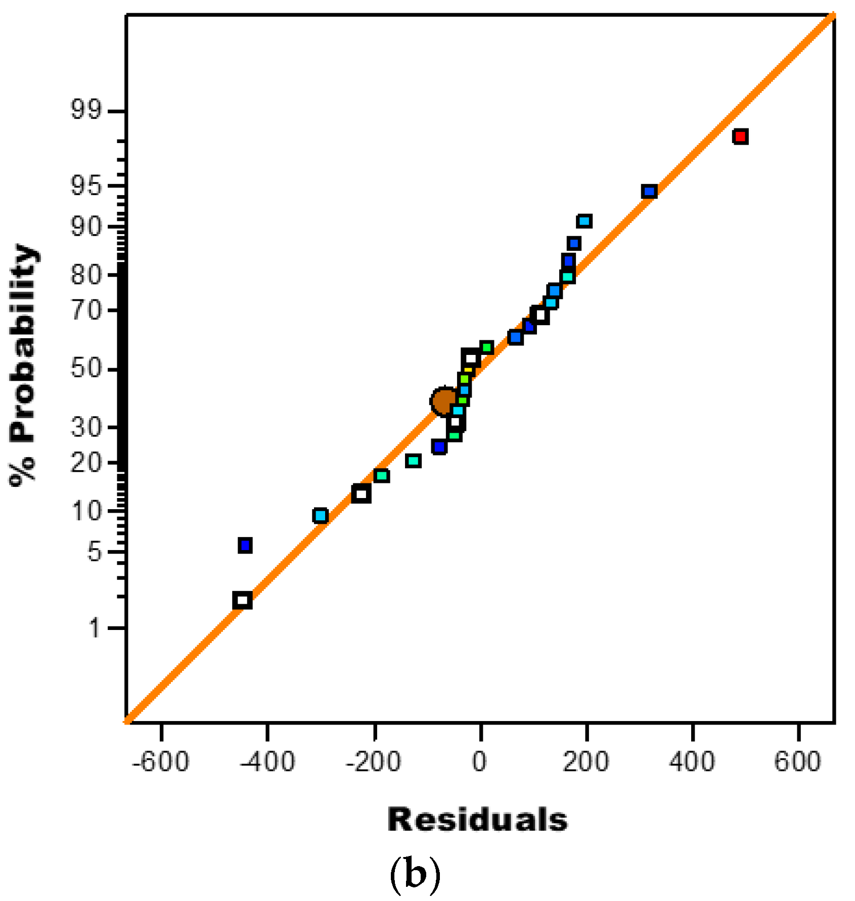
3.3.3. Diagnostic Plots

From Figure 6a,b, the statistical approximations were found in adequate match with CFD predictions, as indicated by a distribution of actual and predicted values closer to the diagonal line for both model responses.

The standard deviation between the actual and predicted data points within the normal distribution range was confirmed by the normal probability plots (Figure 7a,b). Simply, this helps to evaluate the reliability of an empirical model by the outliers or the noise of data points. The more the number of outliers is, the less the model will be effective and reliable. As shown in Figure 6a,b, the data points were distributed rectilinearly without any notable patterns obtained. Therefore, the presently obtained models were adequate at accuracy and could predict responses consistent with real data.

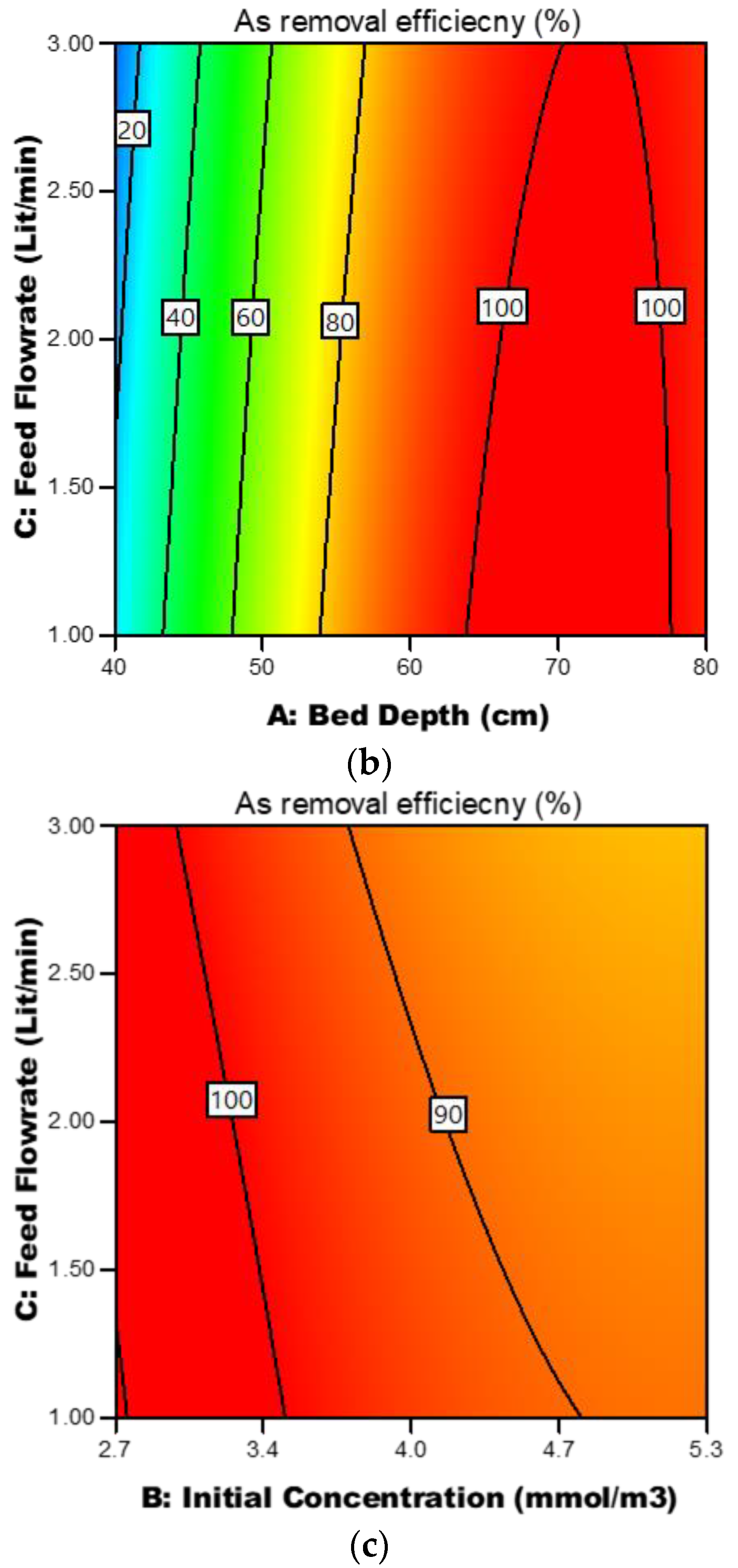
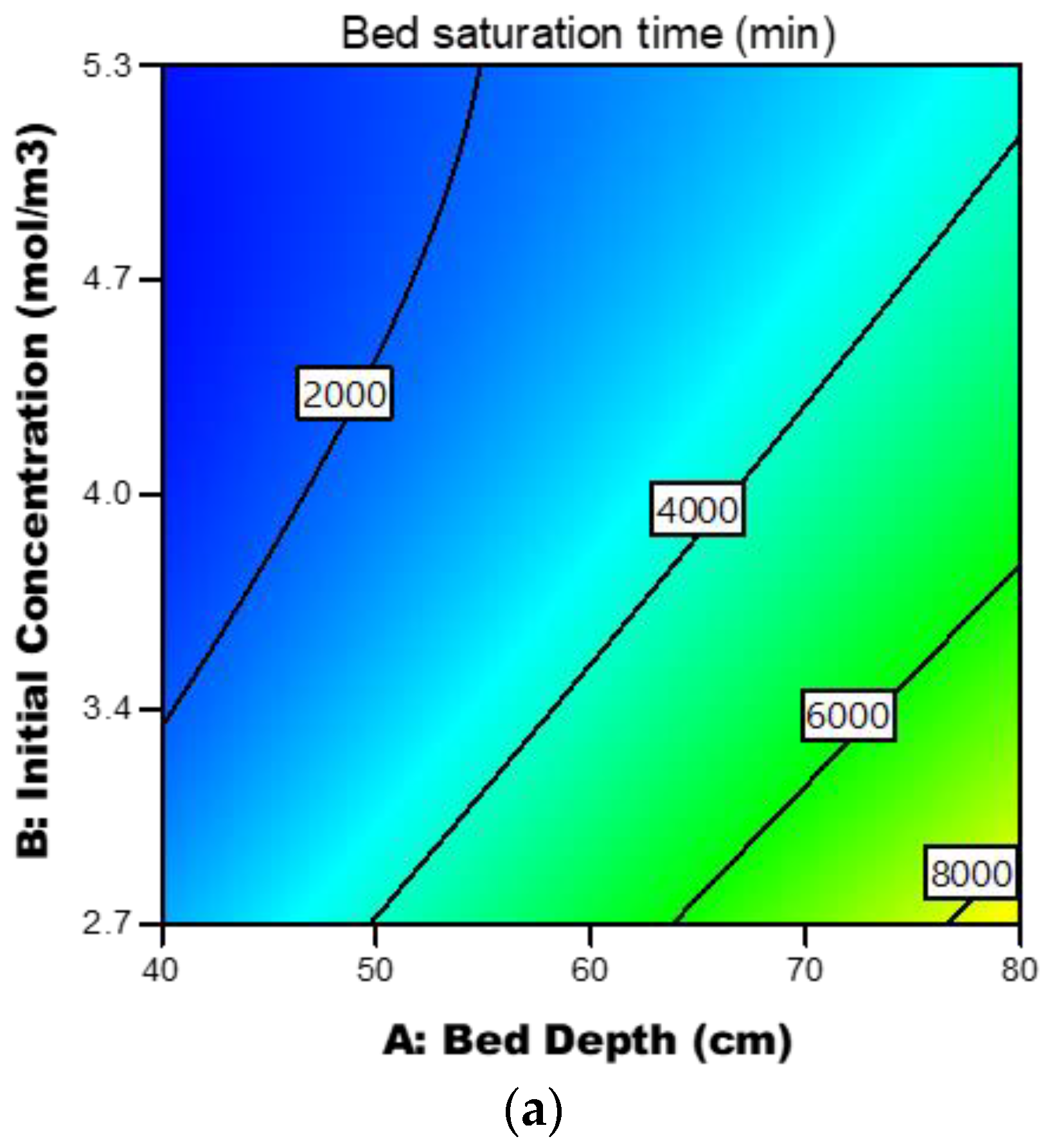
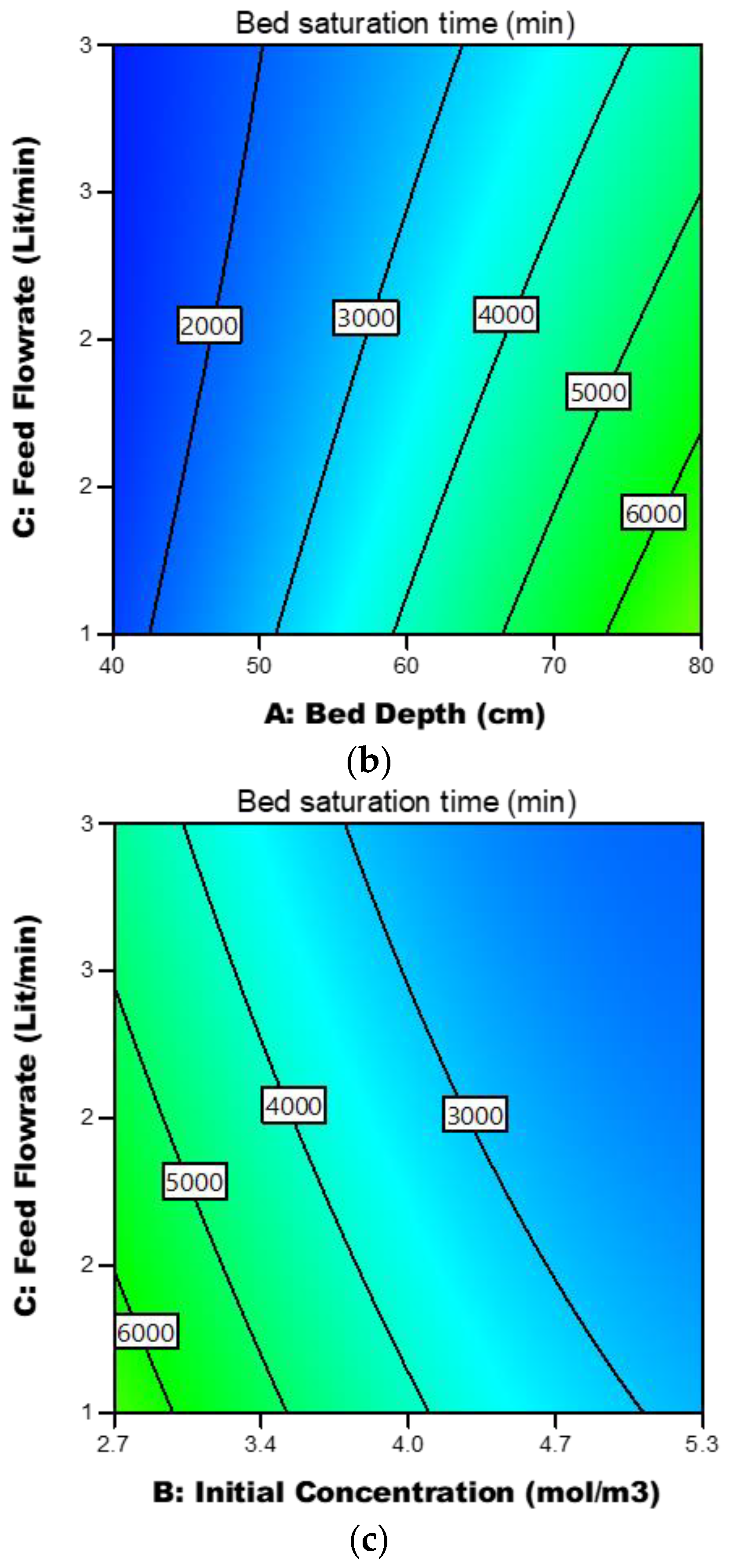
3.3.4. Response Contour Plots

The interaction effects of the bed depth, the initial As conc., and the feed flow rate on the As removal efficiency and the bed saturation time are illustrated in contour plots in Figure 8a–c and Figure 9a–c, respectively, which supported the relationship between responses and the model variables as proposed by regression models. It can be seen that both the As removal efficiency and the bed saturation time were significantly increased by increasing the bed depth whereas the feed flow rate exhibited a negative effect on both responses. In all the plots, it is obvious that, regardless of changing As conc. and the feed flow rate, changing the bed depth remarkably changed both responses. The initial As concentration showed relatively a less effect on both the responses. These findings were substantially consistent with the ANOVA analysis.

4. Conclusions

This work demonstrates an effective approach which combines the use of an experimentally validated CFD model and RSM to simulate and optimize a fixed-bed adsorption process of arsenic (As). The study was started by conducting a few experiments on a small-scale fixed-bed adsorption column for the arsenic removal from wastewater. Subsequently, the COMSOL Multiphysics tool was used to develop the CFD model of the fixed-bed adsorption of arsenic. Finally, the experimentally validated CFD model was combined with RSM to further optimize the design of a lab-scale fixed-bed adsorption process for arsenic. In the RSM, the bed depth, the initial As concentration (conc.), and the feed flow rate were selected as model terms, whereas the As removal efficiency and the bed saturation time were selected as responses. The ANOVA results suggested that quadratic regression models were highly significant for both responses. Moreover, the regression model equations were developed which could desirably predict the responses in terms of selected model parameters and their interaction effects. The CFD predictions were in remarkable match with those measured with the help of developed regression models. The RSM results suggested that compared with those of the initial As conc. and the feed flow rate, the effect of the bed depth was more significant. Moreover, both the As removal efficiency and the bed saturation time were increased reasonably with the increasing bed depth and decreased with the increasing feed flow rate and initial As conc. The optimum conditions for the As removal process were obtained as the bed height of 80 cm, the initial As conc. of 2.7 mmol/m³, and the feed flow rate of 1 L/min. It is expected that findings of the As removal efficiency and the bed saturation time obtained from the combined CFD−RSM approach could be a useful guideline in order to develop and optimize a fixed-bed adsorption process for As removal, which can further be extended for industrial applications.

References

1. Jamil, N.; Baqar, M.; Shaikh, I.A. Assessment of contamination in water and soil surrounding a chlor-alkali plant: A case study. J. Chem. Soc. Pak. 2015, 37, 173–178. [Google Scholar]
2. Raza, A.; Farooq, A.; Ali, W.; Javed, A. Effect of human settlements on surface and groundwater quality: Statistical source identification of heavy and trace metals of siran river and its catchment area mansehra, pakistan. J. Chem. Soc. Pak. 2017, 39, 296–308. [Google Scholar]
3. Yadav, A.; Dindorkar, S.S.; Ramisetti, S.B.; Sinha, N. Simultaneous adsorption of methylene blue and arsenic on graphene, boron nitride and boron carbon nitride nanosheets: Insights from molecular simulations. J. Water Process Eng. 2022, 46, 102653. [Google Scholar] [CrossRef]
4. Ranjan, A. Spatial Analysis of Arsenic Contamination of Groundwater around the World and India. IJISSH 2019, 4, 1–10. [Google Scholar]
5. Wang, Y.-Y.; Chai, L.-Y.; Yang, W.-C. Arsenic distribution and pollution characteristics. In Arsenic Pollution Control in Nonferrous Metallurgy; Springer: Cham, Switzerland, 2019; pp. 1–15. [Google Scholar]
6. Chandrajith, R.; Diyabalanage, S.; Dissanayake, C. Geogenic fluoride and arsenic in groundwater of Sri Lanka and its implications to community health. Groundw. Sustain. Dev. 2020, 10, 100359. [Google Scholar] [CrossRef]
7. Zanini, A.; Petrella, E.; Sanangelantoni, A.M.; Angelo, L.; Ventosi, B.; Viani, L.; Rizzo, P.; Remelli, S.; Bartoli, M.; Bolpagni, R.; et al. Groundwater characterization from an ecological and human perspective: An interdisciplinary approach in the Functional Urban Area of Parma, Italy. Rend. Lincei Sci. Fis. E Nat. 2019, 30, 93–108. [Google Scholar] [CrossRef]
8. Shaban, M.; Abukhadra, M.R.; Rabia, M.; Elkader, Y.A.; Abd El-Halim, M.R. Investigation the adsorption properties of graphene oxide and polyaniline nano/micro structures for efficient removal of toxic Cr(VI) contaminants from aqueous solutions; kinetic and equilibrium studies. Rend. Lincei Sci. Fis. E Nat. 2018, 29, 141–154. [Google Scholar] [CrossRef]
9. Mandal, B.K.; Suzuki, K.T. Arsenic round the world: A review. Talanta 2002, 58, 201–235. [Google Scholar] [CrossRef]
10. Hocaoglu, S.M.; Wakui, Y.; Suzuki, T.M. Separation of arsenic(V) by composite adsorbents of metal oxide nanoparticles immobilized on silica flakes and use of adsorbent coated alumina tubes as an alternative method. J. Water Process Eng. 2019, 27, 134–142. [Google Scholar] [CrossRef]
11. Hashim, M.A.; Kundu, A.; Mukherjee, S.; Ng, Y.-S.; Mukhopadhyay, S.; Redzwan, G.; Sen Gupta, B. Arsenic removal by adsorption on activated carbon in a rotating packed bed. J. Water Process Eng. 2019, 30, 100591. [Google Scholar] [CrossRef]
12. Sujatha, S.; Rajasimman, M. Development of a green emulsion liquid membrane using waste cooking oil as diluent for the extraction of arsenic from aqueous solution—Screening, optimization, kinetics and thermodynamics studies. J. Water Process Eng. 2021, 41, 102055. [Google Scholar] [CrossRef]
13. Asere, T.G.; Stevens, C.V.; Du Laing, G. Use of (modified) natural adsorbents for arsenic remediation: A review. Sci. Total Environ. 2019, 676, 706–720. [Google Scholar] [CrossRef]
14. Ociński, D.; Mazur, P. Highly efficient arsenic sorbent based on residual from water deironing—Sorption mechanisms and column studies. J. Hazard. Mater. 2020, 382, 121062. [Google Scholar] [CrossRef]
15. Syam Babu, D.; Nidheesh, P. A review on electrochemical treatment of arsenic from aqueous medium. Chem. Eng. Commun. 2020, 208, 389–410. [Google Scholar] [CrossRef]
16. Zhang, Y.; Yu, G.; Siddhu, M.A.H.; Masroor, A.; Ali, M.F.; Abdeltawab, A.A.; Chen, X. Effect of impeller on sinking and floating behavior of suspending particle materials in stirred tank: A computational fluid dynamics and factorial design study. Adv. Powder Technol. 2017, 28, 1159–1169. [Google Scholar] [CrossRef]
17. Cheng, S.-J.; Miao, J.-M.; Wu, S.-J. Investigating the effects of operational factors on PEMFC performance based on CFD simulations using a three-level full-factorial design. Renew. Energy 2012, 39, 250–260. [Google Scholar] [CrossRef]
18. Lee, S.; Park, Y.; Kim, J. An evaluation of factors influencing drag coefficient in double-deck tunnels by CFD simulations using factorial design method. J. Wind Eng. Ind. Aerodyn. 2018, 180, 156–167. [Google Scholar] [CrossRef]
19. Jabbari, B.; Jalilnejad, E.; Ghasemzadeh, K.; Iulianelli, A. Modeling and optimization of a membrane gas separation based bioreactor plant for biohydrogen production by CFD–RSM combined method. J. Water Process Eng. 2021, 43, 102288. [Google Scholar] [CrossRef]
20. Awad, A.M.; Hussein, I.A.; Nasser, M.S.; Ghani, S.A.; Mahgoub, A.O. A CFD- RSM study of cuttings transport in non-Newtonian drilling fluids: Impact of operational parameters. J. Pet. Sci. Eng. 2022, 208, 109613. [Google Scholar] [CrossRef]
21. Kola, P.V.K.V.; Pisipaty, S.K.; Mendu, S.S.; Ghosh, R. Optimization of performance parameters of a double pipe heat exchanger with cut twisted tapes using CFD and RSM. Chem. Eng. Process. Process Intensif. 2021, 163, 108362. [Google Scholar] [CrossRef]
22. Singh, S.; Chakraborty, J.P.; Mondal, M.K. Pyrolysis of torrefied biomass: Optimization of process parameters using response surface methodology, characterization, and comparison of properties of pyrolysis oil from raw biomass. J. Clean. Prod. 2020, 272, 122517. [Google Scholar] [CrossRef]
23. Tran, T.V.; Nguyen, H.; Le, P.H.A.; Nguyen, D.T.C.; Nguyen, T.T.; Nguyen, C.V.; Vo, D.-V.N.; Nguyen, T.D. Microwave-assisted solvothermal fabrication of hybrid zeolitic–imidazolate framework (ZIF-8) for optimizing dyes adsorption efficiency using response surface methodology. J. Environ. Chem. Eng. 2020, 8, 104189. [Google Scholar] [CrossRef]
24. Lysova, N.; Solari, F.; Vignali, G. Optimization of an indirect heating process for food fluids through the combined use of CFD and Response Surface Methodology. Food Bioprod. Process. 2022, 131, 60–76. [Google Scholar] [CrossRef]
25. Yaqub, M.; Lee, S.H.; Lee, W. Investigating micellar-enhanced ultrafiltration (MEUF) of mercury and arsenic from aqueous solution using response surface methodology and gene expression programming. Sep. Purif. Technol. 2022, 281, 119880. [Google Scholar] [CrossRef]
26. Gokcek, O.B.; Uzal, N. Arsenic removal by the micellar-enhanced ultrafiltration using response surface methodology. Water Supply 2020, 20, 574–585. [Google Scholar] [CrossRef]
27. Yaqub, M.; Lee, S.H. Experimental and neural network modeling of micellar enhanced ultrafiltration for arsenic removal from aqueous solution. Environ. Eng. Res. 2021, 26, 190261. [Google Scholar] [CrossRef]
28. Baskan, M.B.; Pala, A. Determination of arsenic removal efficiency by ferric ions using response surface methodology. J. Hazard. Mater. 2009, 166, 796–801. [Google Scholar] [CrossRef]
29. Noguchi, H.; Yin, Q.; Lee, S.C.; Xia, T.; Niwa, T.; Lay, W.; Chua, S.C.; Yu, L.; Tay, Y.J.; Nassir, M.J. Performance of Newly Developed Intermittent Aerator for Flat-Sheet Ceramic Membrane in Industrial MBR System. Water 2022, 14, 2286. [Google Scholar] [CrossRef]
30. Mackay, D.M.; Freyberg, D.L.; Roberts, P.V.; Cherry, J.A. A natural gradient experiment on solute transport in a sand aquifer: 1. Approach and overview of plume movement. Water Resour. Res. 1986, 22, 2017–2029. [Google Scholar] [CrossRef]
31. Solangi, Z.A.; Bhatti, I.; Qureshi, K. Modeling and Simulation of Fixed Bed Column for Arsenic Removal using Iron Ore and PAN Fiber Adsorbents. Int. J. Emerg. Technol. 2021, 12, 183–191. [Google Scholar]
32. Nguyen, D.T.C.; Vo, D.-V.N.; Nguyen, T.T.; Nguyen, T.T.T.; Nguyen, L.T.T.; Tran, T.V. Optimization of tetracycline adsorption onto zeolitic–imidazolate framework-based carbon using response surface methodology. Surf. Interfaces 2022, 28, 101549. [Google Scholar] [CrossRef]
33. Hosseinpour, M.; Soltani, M.; Noofeli, A.; Nathwani, J. An optimization study on heavy oil upgrading in supercritical water through the response surface methodology (RSM). Fuel 2020, 271, 117618. [Google Scholar] [CrossRef]
Figure 1. Schematic representation of the experimental setup.
Processes 10 01730 g001
Figure 2. Computational domain of the fixed bed column for numerical simulations: (a) 2D geometry of the fixed-bed adsorption column developed using COMSOL; (b) meshed domain of the developed geometry.
Processes 10 01730 g002
Figure 3. Grid independence test results with simulated cases at a fixed bed depth (40 cm) and a feed flow rate (1 lit/min), but varying feed arsenic concentrations: (a) feed concentration of 2.7 mmol/m3 (a 40 cm bed depth and a 1 lit/min feed flow); (b) feed concentration of 4.0 mmol/m3 (a 40 cm bed depth and a 1 lit/min feed flow); (c) feed concentration of 5.3 mmol/m3 (a 40 cm bed depth and a 1 lit/min feed flow).
Processes 10 01730 g003
Figure 4. Validation of the CFD model with experimental measurements.
Processes 10 01730 g004
Figure 5. Effects of the bed depth, the feed flow rate, and the initial arsenic concentration.
Processes 10 01730 g005
Figure 6. The actual versus predicted plots for the As removal efficiency (a) and the bed saturation time (b).
Processes 10 01730 g006aProcesses 10 01730 g006b
Figure 7. The normal probability plots for the As removal efficiency (a) and the bed saturation time (b).
Processes 10 01730 g007aProcesses 10 01730 g007b
Figure 8. Effects of various parameters on As removal efficiency R1: (a) at a feed flow rate of 2 L/min; (b) at an initial As conc. of 4.0 mmol/m3; (c) at a bed height of 60 cm.
Processes 10 01730 g008aProcesses 10 01730 g008b
Figure 9. Effects of various parameters on bed saturation time R2: (a) at a feed flow rate of 2 L/min; (b) at an initial As conc. of 4.0 mmol/m3; (c) at a bed height of 40 cm.
Processes 10 01730 g009aProcesses 10 01730 g009b