1. Introduction
In general, entropy is considered as a measure of the randomness or disorder of a physical or biological system under intrinsic random fluctuations and environmental disturbances [
1,
2,
3,
4,
5]. According to the second law of thermodynamics, entropy is used to describe the dispersion of energy in a thermally isolated system, in which energy has a natural tendency to spontaneously change toward states with higher entropy [
6,
7,
8]. In order to maintain life, biological systems need to exchange material and energy with their environment in a continual process, so they are open systems [
9].
In this exchange process, the entropy of biological systems can maintain a dynamic balance [
10]. Under such a background, the calculation of biological system entropy is particularly important. In the past few decades, the system entropy in biological networks has been extensively studied [
11,
12,
13]. The discrete-time model plays an important role in numerical calculation, stochastic simulation and numerical analysis [
14,
15,
16,
17,
18]. For continuous-time stochastic systems, the authors of [
16] calculated the system entropy of biological systems from their system matrices by the global linearization technique. In this way, the measurement of the system entropy of nonlinear biological networks could be transformed to solve an optimization problem constrained by a set of LMIs. In this paper, we follow the line of [
16] and extend the LMI method to the calculation of the discrete-time system entropy of stochastic biological networks. With the aid of the Matlab software package, we solve the corresponding LMI-constrained optimization problem to measure the discrete-time system entropy of a nonlinear biological network.
This paper is organized as follows. In
Section 2, we discuss how to calculate the entropy of the discrete-time linear network.
Section 3 gives the system entropy measurement of the discrete-time nonlinear random biological network.
Section 4 presents how to calculate the system entropy in discrete-time nonlinear stochastic biological networks, which is approximated by the global linearization method. Lastly, in
Section 5, an example is given to illustrate the measurement procedure and to validate the feasibility of the proposed system entropy measurement method.
2. System Entropy in Discrete-Time Linear Biological Networks
In this section, we consider a discrete-time linear network, which is described as follows:
where
,
,
,
denotes the biological network’s state vector, random input and output, respectively.
is the finite terminal time.
A,
B and
C are matrices with proper dimensions with the following formats:
The randomness of this system’s output
can be measured by
while the randomness of input signals
is denoted as
where
denotes the expectation. Similar to the definitions of entropy in [
16], the entropy of the input signal or output signal for a discrete-time system is also defined by
and the entropy of
is defined by
Thus, it is natural to define the net signal entropy of a biological system as the discrete-time system entropy, i.e.,
Thus, if the system randomness
r of System (
1) is defined as the following
the system entropy is represented as
In order to calculate the system entropy
s in (
1), we have to calculate or approximate the system randomness first. Of course, it is not easy to approximate such randomness directly. Therefore, we need to estimate the system randomness indirectly as follows:
which is equivalent to
Here, denotes the upper bound of r.
We will decrease the upper bound
to be as small as possible, to approach the randomness
r of the discrete-time biological network (
1), which is suggested in [
16].
Proposition 1. Suppose that a positive definite matrix p > 0 and a positive real number satisfy the following inequality: Then, is an upper bound of the system randomness of network (1). Proof. Choose the Lyapunov function
, then
Taking summation, and then taking expectation on both sides, we have
Recalling that
,
and
, we have
Completing the square on the right side, we obtain
where the notation
denotes
with
. By inequality (
4), there exists
This shows that the randomness
r of System (
1) has an upper bound
. □
By the Schur lemma, we know that the matrix inequality (
4) equals the following LMI:
Thus, we can obtain the following corollary described by LMI (
5).
Corollary 1. Suppose that there exists a positive definite matrix p > 0 and a positive real number that satisfy the inequality (5); then, is an upper bound of the system randomness of network (1). Remark 1. Compared with the results of Reference [16], the matrix inequality (4) that is obtained by the completing square method is different to the results of Proposition 2 of [16]. Moreover, the structure of LMI (5) for a discrete-time network is different to that of (12) for the continuous-time system discussed in [16]. From Equation (
3), we can see that the upper bound of the discrete-time system randomness
r is
, i.e.,
. Thus, the calculation of the system randomness of network (
1) can be estimated by the following problem:
with the constraint of LMI (
5), where
p > 0.
Based on (
6), with the aid of Matlab’s LMI toolbox, we can decrease
by the constraint of LMI in (
5) until there is no positive matrix
P appearing; then, the above LMI-constrained optimization problem can be solved, and the system randomness
r can be estimated. Thus, the discrete-time system entropy of the linear stochastic System (
1) can be obtained as
. Moreover, the measurement of the system randomness
r or system entropy
s is dependent on matrices
A,
B and
C in System (
1) to some extent.
3. System Entropy in Discrete-Time Nonlinear Network
Nonlinear dynamic systems play an important role in biological networks, which causes the difficulty of estimating the entropy of such systems. Under this situation, the global linearized method is suggested [
19,
20,
21,
22,
23,
24,
25,
26,
27], which is an interpolation method of local linearized systems of a nonlinear biological network. Suppose that the biological systems are described by the following discrete-time nonlinear stochastic biological network:
where
,
f is a function,
denotes
m external input signal and
denotes
m nonlinear couplings between the biological network and environment.
denotes
l nonlinear outputs.
Based on the ideas of the discrete-time system randomness of (
3), we obtain the following proposition.
Proposition 2. Suppose that there exists a positive definite matrix p > 0 and a positive real number that satisfy the following HJI: Then, is an upper bound of the system randomness of network (7). Proof. Let
, then
Taking summation, and then taking expectation on both sides, we obtain
Recalling that
,
and
, we have
Completing the square on the right side, we obtain
where the notation
denotes
with
. By inequality (
8), there exists
This ends the proof. □
Remark 2. Compared with the results of Proposition 4 in Reference [16], the HJI (8) in this paper does not depend on the input variables , but the HJIs in Proposition 4 of [16] include . Thus, the system randomness of network (7) can be obtained only by the coefficients , and , which is defined on the state space. By Proposition 2, the system randomness
r of network (
7) can be approximated to solve the following optimization constrained by HJI:
It is constrained by HJI in (
8), where
p > 0. Denote
The system randomness
r of network (
7) could be estimated by solving the following optimization:
with the constraint of HJI in (
8).
Based on the above results, it is easy to obtain the system entropy as
We can obtain the system randomness
r from the
HJI-constrained optimization problem in (
10) or (
11). However, at present, there exists no efficient method to solve the HJI in (
10) or (
11) analytically or numerically. In this study, the global linearization method in [
21,
27] will be employed to interpolate several local linearized systems at the
M matrices of the convex hull of the globalization systems to approach the nonlinear discrete-time biological systems in (
7), to transform the difficult HJI-constrained optimization problem in (
10) or (
11) to an equivalent LMIs-constrained optimization problem for the calculation of system randomness in the following section.
4. The Global Linearization Method to Estimate System Entropy for Nonlinear Networks
In this section, the global linearization technique is suggested to help in estimating the system entropy of nonlinear stochastic systems in (
7). The main idea of this method is described as follows: we convert the nonlinear system into a set of interpolated locally linearized networks in which the linear system’s entropy is easy to calculate and approximate [
16,
21,
27]. Therefore, the estimation of system randomness and entropy can be transformed to solve the
HJI-constrained optimization problems (
10) efficiently.
We prefer the detailed theory of the global linearization method to Reference [
21]. According to this method, the global linearized systems are constructed by the convex hull of
M vertices defined in Equation (
12) as follows:
Then, the state
in the discrete-time nonlinear System (
7) can be represented by those states of local linearized biological networks with (
12) as follows:
Thus, the combination of linearized systems in (
13) can be represented as:
where the interpolation function (for
)
and
for some
satisfy
and
, while
denotes the
ith local operation point with local linearization [
27], i.e., the trajectory of the nonlinear System (
7) can be represented by the trajectories of the interpolated biological network in (
14).
If the nonlinear biological network in Equation (
7) could be approximated by the global linearization system in Equation (
14), then we obtain the following result.
Proposition 3. Suppose that a positive definite matrix p
> 0 and a real number satisfy the following LIMs:
Then, is an upper bound of the system randomness of network (7). Proof. Let Lyapunov function
, and the approximation of
and
are
and
Thus, we obtain the following result:
where
,
,
.
This ends the proof. □
Based on this technique, the system randomness
r of network (
7) or (
14) can be approximated by solving the following optimization problem:
with the constraint of LMIs in (
16) and
p > 0. The system randomness
r in (
18) could be obtained by decreasing its upper bound
until there exists no
p > 0.
5. Example and Simulation
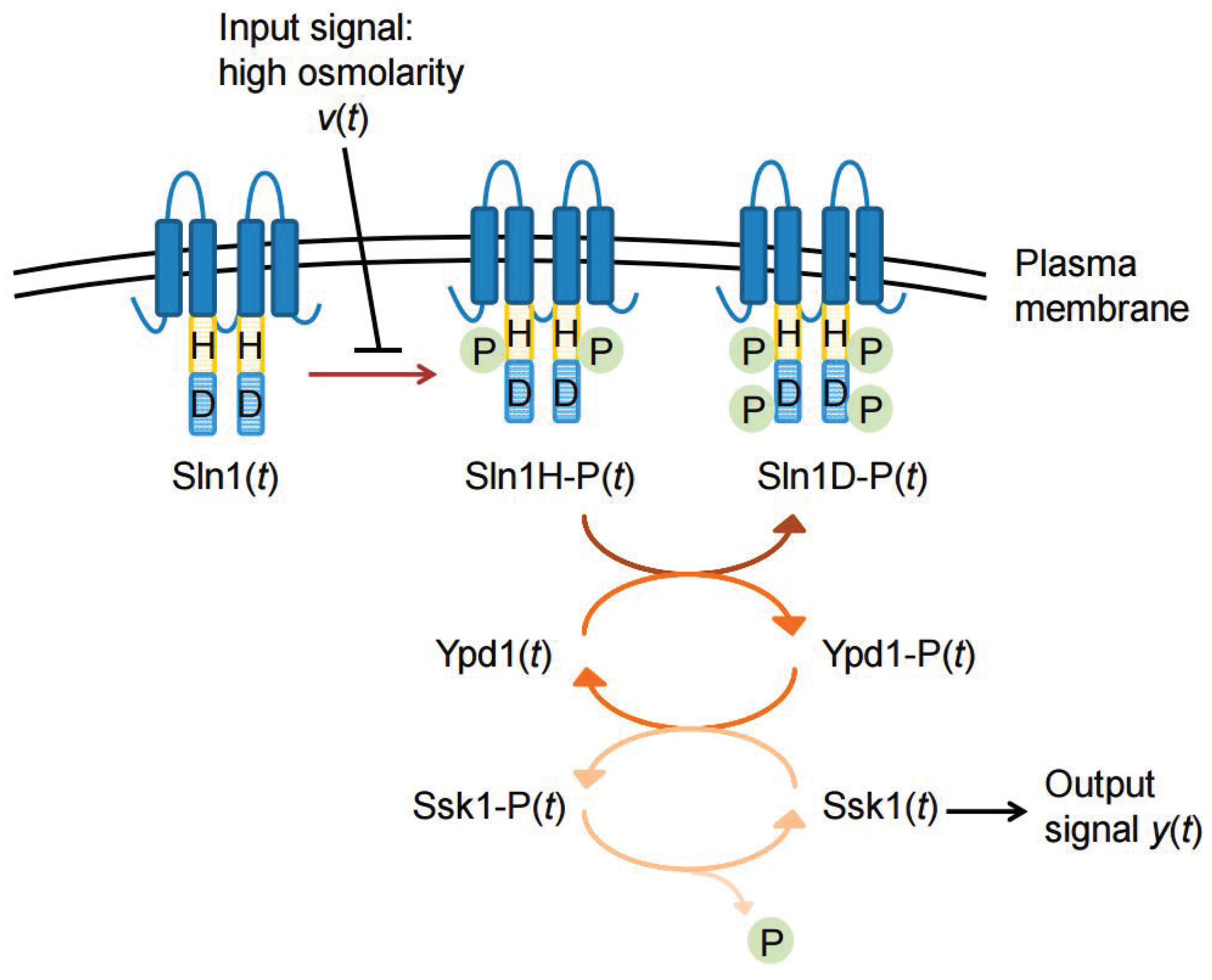
In this section, we consider a phosphorelay system in yeast, discussed in [
16,
23]; see
Figure 1. This signal transduction pathway includes seven state variables: Sln1, Sln1H-P, Sln1D-P, Ypd1, Yod1-P, Ssk1, Ssk1-P. We prefer to References [
16,
23,
25], for detailed information.
The state
is denoted by the following vector:
Suppose that the dynamic behavior of this system can be represented by discrete-time difference equations, which are seen as the discrete-time type of phosphorelay system discussed in [
25]:
where
and
are the systematic characteristics, and
is the random fluctuation.
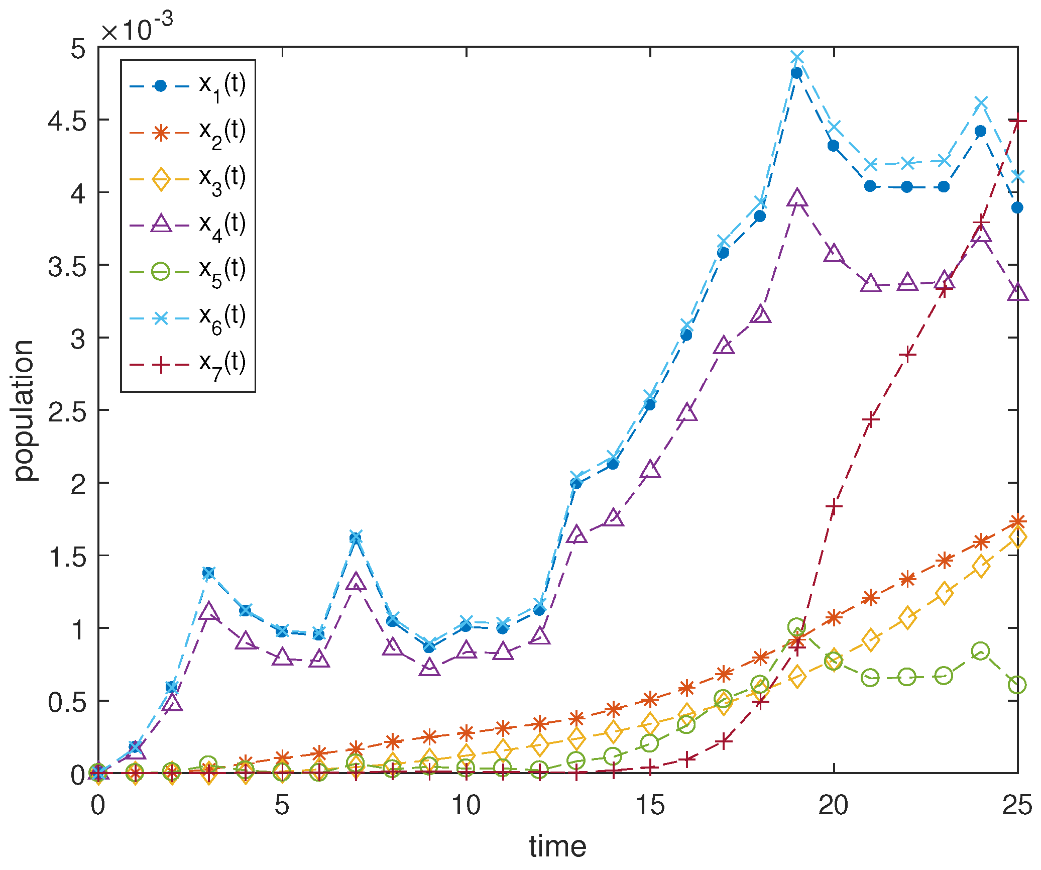
Figure 2 shows the trajectories of
x with the systematic characteristics
and
, which is the standard Gaussian white noise with zero mean.
In order to show the effects of systematic characteristics on system entropy, we take the three different systematic characteristics given in
Table 1.
Due to the global linearization in (
14), the approximation of discrete-time nonlinear network (
20) can be presented by:
where
denotes the the interpolation functions.
denotes the
M states of local linearization systems [
26].
By solving the LMI-constrained optimization problem in Equation (
18) for the above three system characteristic cases in
Table 1, the positive definite matrices
,
and
are obtained as follows:
Corresponding system entropy is calculated, and the result is shown in following
Table 2.
By the estimation results of
Table 2, we see that the different systematic characteristics in (
20) can affect the system entropy of the biological network.


