
Descriptor Representation-Based Guaranteed Cost Control Design Methodology for Polynomial Fuzzy Systems


Abstract
:1. Introduction
- A descriptor representation-based methodology is proposed for the GCC design of PFM;
- The operation domain is considered in the proposed GCC design for solving the negative highest order term infeasible issue, which frequently happens in the SOS-based GCC design of [43];
- The fuzzy slack matrices are applied to descriptor representation-based GCC design for relaxation.
2. Descriptor Representation of the Closed-Loop Polynomial Fuzzy System
3. Guaranteed Cost Control Design
4. Design Examples
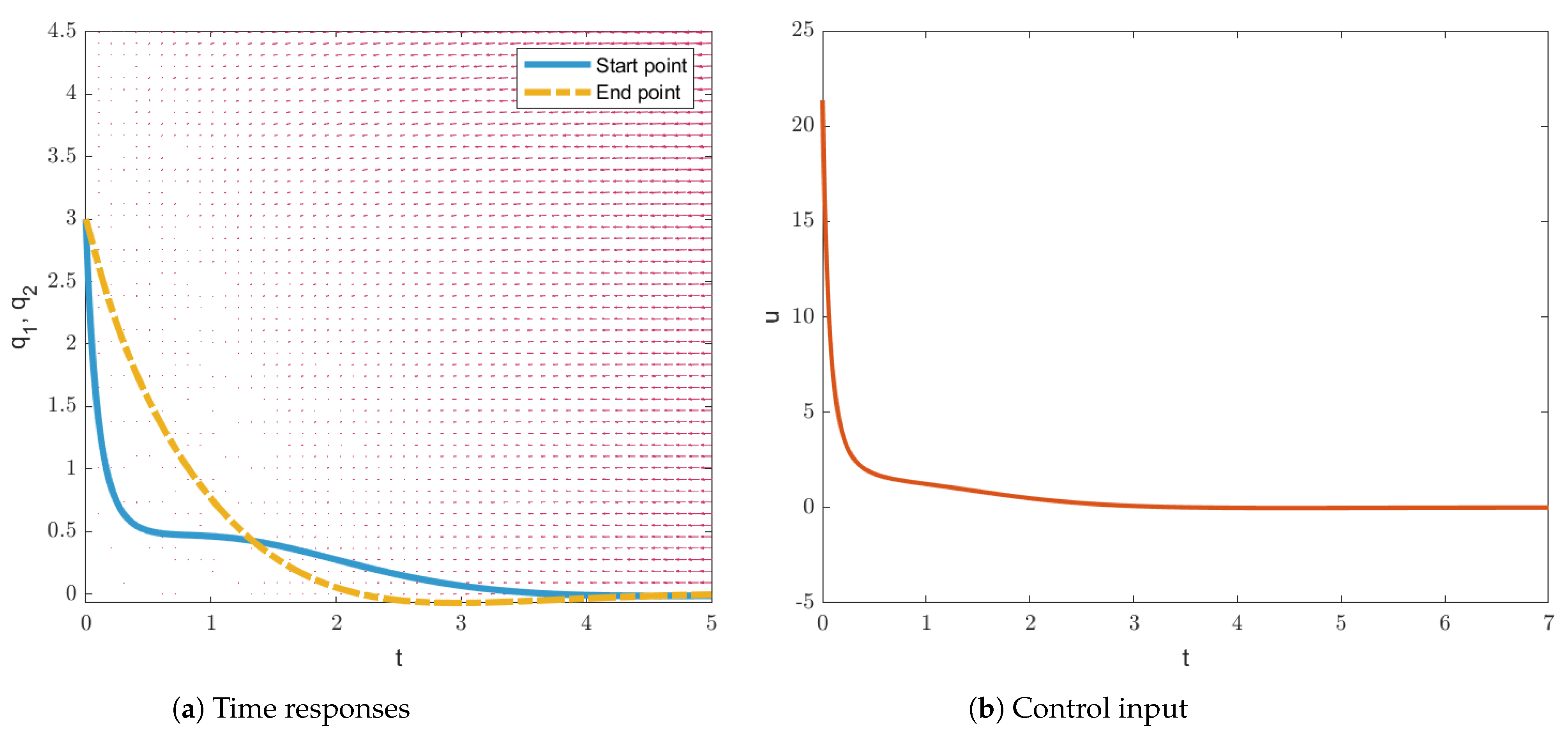
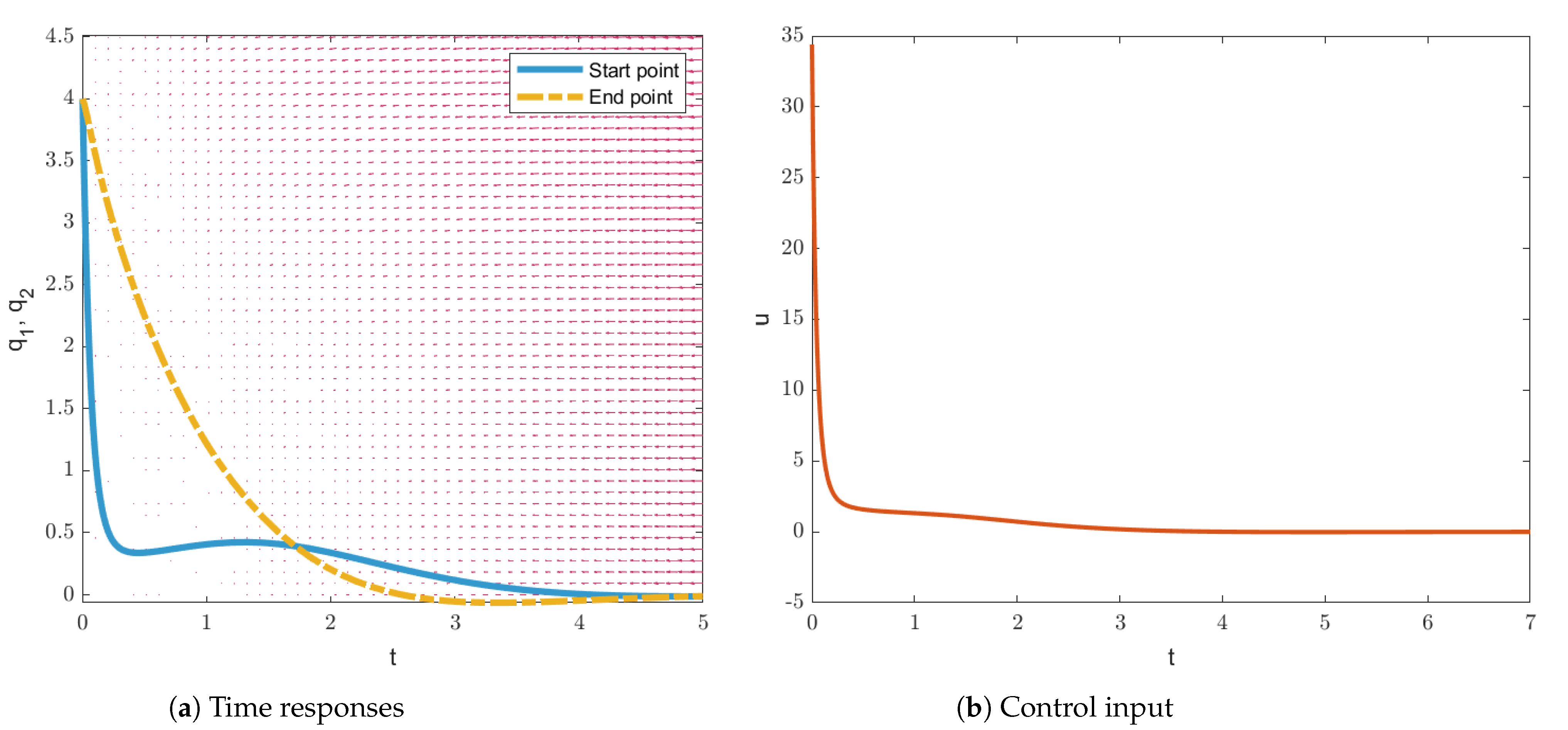
4.1. Example 1
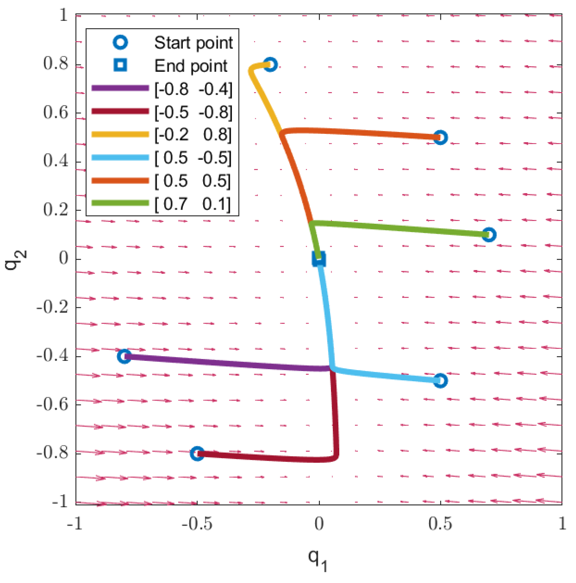
4.2. Example 2
5. Conclusions
Author Contributions
Funding
Institutional Review Board Statement
Informed Consent Statement
Data Availability Statement
Conflicts of Interest
References
- Takagi, T.; Sugeno, M. Fuzzy identification of systems and its applications to modeling and control. IEEE Trans. Syst. Man Cybern. B Cybern. 1985, SMC-15, 116–132. [Google Scholar] [CrossRef]
- Wu, H.; Li, H. Finite-Dimensional Constrained Fuzzy Control for a Class of Nonlinear Distributed Process Systems. IEEE Trans. Syst. Man Cybern. B Cybern. 2007, 37, 1422–1430. [Google Scholar] [CrossRef]
- Chen, Y.; Ohtake, H.; Tanaka, K.; Wang, W.; Wang, H.O. Relaxed Stabilization Criterion for T–S Fuzzy Systems by Minimum-Type Piecewise-Lyapunov-Function-Based Switching Fuzzy Controller. IEEE Trans. Fuzzy Syst. 2012, 20, 1166–1173. [Google Scholar] [CrossRef]
- Vu, V.P.; Wang, W.J. Robust observer synthesis for the uncertain large-scale T–S fuzzy system. IET Control Theory Appl. 2019, 13, 134–145. [Google Scholar] [CrossRef]
- Wang, H.O.; Tanaka, K.; Griffin, M.F. An approach to fuzzy control of nonlinear systems: Stability and design issues. IEEE Trans. Fuzzy Syst. 1996, 4, 14–23. [Google Scholar] [CrossRef]
- Feng, G. A Survey on Analysis and Design of Model-Based Fuzzy Control Systems. IEEE Trans. Fuzzy Syst. 2006, 14, 676–697. [Google Scholar] [CrossRef]
- Tanaka, K.; Wang, H.O. Fuzzy Control Systems Design and Analysis: A Linear Matrix Inequality Approach; Wiley: New York, NY, USA, 2001. [Google Scholar]
- Tanaka, K.; Ohtake, H.; Wang, H.O. A Descriptor System Approach to Fuzzy Control System Design via Fuzzy Lyapunov Functions. IEEE Trans. Fuzzy Syst. 2007, 15, 333–341. [Google Scholar] [CrossRef]
- Guelton, K.; Bouarar, T.; Manamanni, N. Robust dynamic output feedback fuzzy Lyapunov stabilization of Takagi-Sugeno systems—A descriptor redundancy approach. Fuzzy Sets Syst. 2009, 160, 2796–2811. [Google Scholar] [CrossRef]
- Chadli, M.; Aouaouda, S.; Karimi, H.R.; Shi, P. Robust fault tolerant tracking controller design for a VTOL aircraft. J. Frankl. Inst. 2013, 350, 2627–2645. [Google Scholar] [CrossRef]
- Aouaouda, S.; Chadli, M.; Karimi, H.R. Robust static output-feedback controller design against sensor failure for vehicle dynamics. IET Control Theory Appl. 2014, 8, 728–737. [Google Scholar] [CrossRef]
- Tanaka, K.; Yoshida, H.; Ohtake, H.; Wang, H.O. A Sum-of-Squares Approach to Modeling and Control of Nonlinear Dynamical Systems With Polynomial Fuzzy Systems. IEEE Trans. Fuzzy Syst. 2009, 17, 911–922. [Google Scholar] [CrossRef]
- Sala, A.; AriÑo, C. Polynomial Fuzzy Models for Nonlinear Control: A Taylor Series Approach. IEEE Trans. Fuzzy Syst. 2009, 17, 1284–1295. [Google Scholar] [CrossRef]
- Narimani, M.; Lam, H.K. SOS-Based Stability Analysis of Polynomial Fuzzy-Model-Based Control Systems Via Polynomial Membership Functions. IEEE Trans. Fuzzy Syst. 2010, 18, 862–871. [Google Scholar] [CrossRef]
- Chen, Y.J.; Tanaka, M.; Tanaka, K.; Ohtake, H.; Wang, H.O. Discrete polynomial fuzzy systems control. IET Control Theory Appl. 2014, 8, 288–296. [Google Scholar] [CrossRef]
- Vu, V.P.; Wang, W.J. Polynomial Controller Synthesis for Uncertain Large-Scale Polynomial T–S Fuzzy Systems. IEEE Trans. Cybern. 2021, 51, 1929–1942. [Google Scholar] [CrossRef] [PubMed]
- Vu, V.P.; Wang, W.J. Decentralized Observer-Based Controller Synthesis for a Large-Scale Polynomial T–S Fuzzy System With Nonlinear Interconnection Terms. IEEE Trans. Cybern. 2021, 51, 3312–3324. [Google Scholar] [CrossRef] [PubMed]
- Tsai, S.H.; Wang, J.W.; Song, E.S.; Lam, H.K. Robust H∞ Control for Nonlinear Hyperbolic PDE Systems Based on the Polynomial Fuzzy Model. IEEE Trans. Cybern. 2021, 51, 3789–3801. [Google Scholar] [CrossRef]
- Chen, Y.J.; Tanaka, K.; Tanaka, M.; Tsai, S.H.; Wang, H.O. A Novel Path-Following-Method-Based Polynomial Fuzzy Control Design. IEEE Trans. Cybern. 2021, 51, 2993–3003. [Google Scholar] [CrossRef]
- Xiao, B.; Lam, H.K.; Zhou, H.; Gao, J. Analysis and Design of Interval Type-2 Polynomial-Fuzzy-Model-Based Networked Tracking Control Systems. IEEE Trans. Fuzzy Syst. 2021, 29, 2750–2759. [Google Scholar] [CrossRef]
- Fu, L.; Lam, H.K.; Liu, F.; Xiao, B.; Zhong, Z. Static Output-Feedback Tracking Control for Positive Polynomial Fuzzy Systems. IEEE Trans. Fuzzy Syst. 2022, 30, 1722–1733. [Google Scholar] [CrossRef]
- Yu, G.R.; Chiu, Y.S.; Huang, L.W. Polynomial Fuzzy Control of an Underactuated Robot Using Sum of Squares. In Proceedings of the 12th Asian Control Conference (ASCC), Kitakyushu, Japan, 9–12 June 2019; pp. 895–900. [Google Scholar]
- Lam, H.K.; Lo, J.C. Output Regulation of Polynomial-Fuzzy-Model-Based Control Systems. IEEE Trans. Fuzzy Syst. 2013, 21, 262–274. [Google Scholar] [CrossRef]
- Zhao, Y.; He, Y.; Feng, Z.; Shi, P.; Du, X. Relaxed Sum-of-Squares Based Stabilization Conditions for Polynomial Fuzzy-Model-Based Control Systems. IEEE Trans. Fuzzy Syst. 2019, 27, 1767–1778. [Google Scholar] [CrossRef]
- Meng, A.; Lam, H.K.; Liu, F.; Zhang, C.; Qi, P. Output Feedback and Stability Analysis of Positive Polynomial Fuzzy Systems. IEEE Trans. Syst. Man Cybern. B Cybern. 2021, 51, 7707–7718. [Google Scholar] [CrossRef]
- Han, M.; Lam, H.K.; Li, Y.; Liu, F.; Zhang, C. Observer-based control of positive polynomial fuzzy systems with unknown time delay. Neurocomputing 2019, 349, 77–90. [Google Scholar] [CrossRef]
- Khooban, M.H.; Vafamand, N.; Dragičević, T.; Blaabjerg, F. Polynomial fuzzy model-based approach for underactuated surface vessels. IET Control Theory Appl. 2018, 12, 914–921. [Google Scholar] [CrossRef]
- Yu, F.N.; Chen, Y.J.; Tanaka, M.; Tanaka, K.; Tsai, S.-H. Descriptor Form Design Methodology for Polynomial Fuzzy-Model-Based Control Systems. Int. J. Fuzzy Syst. 2022, 24, 841–854. [Google Scholar] [CrossRef]
- Liu, J.; Wei, L.; Cao, J.; Fei, S. Hybrid-driven H∞ filter design for T–S fuzzy systems with quantization. Nonlinear Anal. Hybrid Syst. 2019, 31, 135–152. [Google Scholar] [CrossRef]
- Tsai, S.H.; Jen, C.Y. H∞ Stabilization for Polynomial Fuzzy Time-Delay System: A Sum-of-Squares Approach. IEEE Trans. Fuzzy Syst. 2018, 26, 3630–3644. [Google Scholar] [CrossRef]
- Teng, L.; Wang, Y.; Cai, W.; Li, H. Robust Fuzzy Model Predictive Control of Discrete-Time Takagi–Sugeno Systems With Nonlinear Local Models. IEEE Trans. Fuzzy Syst. 2018, 26, 2915–2925. [Google Scholar] [CrossRef]
- Yang, W.; Feng, G.; Zhang, T. Robust Model Predictive Control for Discrete-Time Takagi–Sugeno Fuzzy Systems With Structured Uncertainties and Persistent Disturbances. IEEE Trans. Fuzzy Syst. 2014, 22, 1213–1228. [Google Scholar] [CrossRef]
- Tanaka, K.; Tanaka, M.; Chen, Y.J.; Wang, H.O. A New Sum-of-Squares Design Framework for Robust Control of Polynomial Fuzzy Systems With Uncertainties. IEEE Trans. Fuzzy Syst. 2016, 24, 94–110. [Google Scholar] [CrossRef]
- Li, H.; Wang, J.; Du, H.; Karimi, H.R. Adaptive Sliding Mode Control for Takagi–Sugeno Fuzzy Systems and Its Applications. IEEE Trans. Fuzzy Syst. 2018, 26, 531–542. [Google Scholar] [CrossRef]
- Chen, C.; Xu, J.; Lin, G. Fuzzy adaptive control particle swarm optimization based on T-S fuzzy model of maglev vehicle suspension system. J. Mech. Sci. Technol. 2020, 34, 43–54. [Google Scholar] [CrossRef]
- de Sousa, M.A.T.; Madrid, M.K. Optimization of Takagi-Sugeno fuzzy controllers using a genetic algorithm. In Proceedings of the Ninth IEEE International Conference on Fuzzy Systems, San Antonio, TX, USA, 7–10 May 2000; pp. 30–35. [Google Scholar]
- Wang, F.; Wang, H.; Zhang, Y.; Guo, X. T-S Fuzzy-Based Optimal Control for Minimally Invasive Robotic Surgery with Input Saturation. J. Sens. 2018. [Google Scholar] [CrossRef]
- Kumaresan, N. Optimal Control for Stochastic Singular Integro-Differential Takagi-Sugeno Fuzzy System Using Ant Colony Programming. Filomat 2012, 26, 415–426. [Google Scholar] [CrossRef]
- Zhang, H.; Liang, Y.; Su, H.; Liu, C. Event-Driven Guaranteed Cost Control Design for Nonlinear Systems With Actuator Faults via Reinforcement Learning Algorithm. IEEE Trans. Fuzzy Syst. 2020, 50, 4135–4150. [Google Scholar] [CrossRef]
- Yan, H.; Zhang, H.; Yang, F.; Zhan, X.; Peng, C. Event-Triggered Asynchronous Guaranteed Cost Control for Markov Jump Discrete-Time Neural Networks With Distributed Delay and Channel Fading. IEEE Trans. Neural Netw. Learn. Syst. 2018, 29, 3588–3598. [Google Scholar] [PubMed]
- Zeng, T.; Ren, X.; Zhang, Y.; Li, G.; Na, J. An Integrated Optimal Design for Guaranteed Cost Control of Motor Driving System With Uncertainty. IEEE/ASME Trans. Mechatron. 2019, 24, 2606–2615. [Google Scholar] [CrossRef]
- Wu, Z.G.; Dong, S.; Shi, P.; Su, H.; Huang, T.; Lu, R. Fuzzy-Model-Based Nonfragile Guaranteed Cost Control of Nonlinear Markov Jump Systems. IEEE Trans. Syst. Man Cybern. B Cybern. 2017, 47, 2388–2397. [Google Scholar] [CrossRef]
- Tanaka, K.; Ohtake, H.; Wang, H.O. Guaranteed Cost Control of Polynomial Fuzzy Systems via a Sum of Squares Approach. IEEE Trans. Syst. Man Cybern. B Cybern. 2009, 39, 561–567. [Google Scholar] [CrossRef]
- Sun, C.; Wang, W.; Chen, Y. A descriptor system approach to fuzzy guaranteed cost control system design. In Proceedings of the 2009 IEEE International Conference on Fuzzy Systems, Jeju, Korea, 20–24 August 2009; pp. 1288–1293. [Google Scholar]
- Prajna, S.; Papachristodoulou, A.; Wu, F. Nonlinear control synthesis by sum of squares optimization: A Lyapunov-based approach. In Proceedings of the 5th Asian Control Conference, Melbourne, VIC, Australia, 20–23 July 2004; pp. 157–165. [Google Scholar]


| Initial Condition | Cost Function Value J of Theorem 1 of [43] | Cost Function Value J of The Proposed Theorem 1 |
|---|---|---|
| 32.81 | 26.60 | |
| 60.79 | 41.94 |
| Initial Condition | Cost Function Value J |
|---|---|
| 0.1245 | |
| 0.1663 | |
| 0.1052 | |
| 0.1677 | |
| 0.0234 | |
| 0.0230 |
| Initial Condition | Cost Function Value J |
|---|---|
| 0.0602 | |
| 0.1747 | |
| 0.0401 | |
| 0.0130 | |
| 0.0215 | |
| 0.0228 |
Publisher’s Note: MDPI stays neutral with regard to jurisdictional claims in published maps and institutional affiliations. |
© 2022 by the authors. Licensee MDPI, Basel, Switzerland. This article is an open access article distributed under the terms and conditions of the Creative Commons Attribution (CC BY) license (https://creativecommons.org/licenses/by/4.0/).
Share and Cite
Shen, Y.-H.; Chen, Y.-J.; Yu, F.-N.; Wang, W.-J.; Tanaka, K. Descriptor Representation-Based Guaranteed Cost Control Design Methodology for Polynomial Fuzzy Systems. Processes 2022, 10, 1799. https://doi.org/10.3390/pr10091799
Shen Y-H, Chen Y-J, Yu F-N, Wang W-J, Tanaka K. Descriptor Representation-Based Guaranteed Cost Control Design Methodology for Polynomial Fuzzy Systems. Processes. 2022; 10(9):1799. https://doi.org/10.3390/pr10091799
Chicago/Turabian StyleShen, Yu-Hsuan, Ying-Jen Chen, Fan-Nong Yu, Wen-June Wang, and Kazuo Tanaka. 2022. "Descriptor Representation-Based Guaranteed Cost Control Design Methodology for Polynomial Fuzzy Systems" Processes 10, no. 9: 1799. https://doi.org/10.3390/pr10091799
APA StyleShen, Y.-H., Chen, Y.-J., Yu, F.-N., Wang, W.-J., & Tanaka, K. (2022). Descriptor Representation-Based Guaranteed Cost Control Design Methodology for Polynomial Fuzzy Systems. Processes, 10(9), 1799. https://doi.org/10.3390/pr10091799