Integrating Dynamic Economic Optimization and Nonlinear Closed-Loop GPC: Application to a WWTP

Abstract

In this paper, a technique that integrates methods of dynamic economic optimization and real-time control by including economic model predictive control and closed-loop predictive control has been developed, using a two-layer structure. The upper layer, which consists of an economic nonlinear MPC (NMPC), makes use of the updated state information to optimize some economic cost indices and calculates in real time the economically optimal trajectories for the process states. The lower layer uses a closed-loop nonlinear GPC (NCLGPC) to calculate the control actions that allow for the outputs of the process to follow the trajectories received from the upper layer. This paper also includes the theoretical demonstration proving that the deviation between the state of the closed-loop system and the economically time varying trajectory provided by the upper layer is bounded, thus guaranteeing stability. The proposed approach is based on the use of nonlinear models to describe all the relevant process dynamics and cover a wide operating range, providing accurate predictions and guaranteeing the performance of the control systems. In particular, the methodology is implemented in the N-Removal process of a WWTP and the results demonstrate that the method is effective and can be used profitably in practical cases such as the chemical, refinery and petrochemical process industries.

1. Introduction

Nowadays, modern industrial processes have become highly integrated with respect to material and energy flows, tightly constrained by high-quality product specifications, and subjected to increasingly strict safety and environmental regulations. These more rigorous operating circumstances have placed new constraints on the operating flexibility of industrial processes and made the performance requirements for process plants increasingly difficult to satisfy. The increased emphasis placed on safe and efficient plant operation dictates the need for continuous monitoring of the operation of a chemical plant and effective external intervention (control) to guarantee satisfaction of the operational objectives. In this light, it is natural that the subject of process control has become increasingly important in both the academic and industrial communities.

Maximizing profit has been and will always be the primary purpose of the optimal control and operation of processes. There are various modern techniques that integrate and seek to guarantee optimization and control simultaneously, and that allow industrial processes to be highly competitive, profitable, operationally safe and beneficial to the environment. Among the most representative techniques are Real-Time Optimization (RTO) and Dynamic Real-Time Optimization (D-RTO). The benefits of RTO are demonstrated by its successful implementation in a number of industrial applications leading to significant economic profits [1]. RTO is suggested when significant changes occur in the operating conditions that closely affect the plant’s profit margin. In large plants, seasonal and day-to-night variations may be sufficient to justify RTO [2]. Within process control, there have been several calls for the integration of MPC and the economic optimization of processes (e.g., refs. [3,4,5]).

In the literature, two-stage MPC structures (refs. [6,7,8]) have been investigated to take into account different slow and fast dynamical of processes using multilayer architectures. There also been also attempts to integrate RTO and nonlinear MPC in a single level [9]. In this approach, the economic optimization and control problems are solved simultaneously in a single layer. In particular model-based predictive control techniques can be formulated to perform both functions by adding economic objective terms to be the standard MPC objective function [9,10]. The resulting problem involves solving a nonlinear optimization problem subject to dynamic and steady-state constraints. The implementation of the extended controller relies on extensive tuning of the weighting factors for stability and performance. Extensive simulations are needed to select appropriate values for the weighting factors [10], unlike in linear MPC where robust tuning techniques are available. The one-layer approach could respond to changes in the plant’s optimal conditions faster than the two-layer approach. However, for large-scale and highly nonlinear processes, this technique may struggle due to computational limitations.

Nevertheless, there is an obvious need for model-based process operation strategies that support the dynamic nonlinear behavior of production plants. More recent techniques, such as dynamic trajectory optimization and nonlinear model predictive control (NMPC), are still subject to research, and, often, the size of the applicable process model is still a limiting factor. In ref. [11], two economically oriented nonlinear MPC formulations were proposed for cyclic processes and the nominal stability of the closed-loop system was established via Lyapunov techniques. In [12], the authors design a Lyapunov-based economic MPC that is capable of optimizing closed-loop performance with respect to general economic considerations for nonlinear systems. The design of this controller is based on uniting receding horizon control with explicit Lyapunov-based nonlinear controller design techniques and allows for an explicit characterization of the stability region of the closed-loop system; such a characterization may be conservative in certain applications and it may be possible for the controller to achieve closed-loop stability for initial conditions outside of the estimated stability region. The MPC schemes in [12] optimize a cost function which is related directly to certain economic considerations and is not necessarily dependent on a steady stat unlike conventional MPC designs. The benefits of two-layer optimization are demonstrated by its successful implementation in a number of industrial applications, leading to significant economical profits. The RTO is recommended when significant changes occur in the operating conditions, strongly affecting the plant profitability. In large plants, seasonal and day-to-night variations may be sufficient to justify RTO. Additionally, the temporal decomposition is a solution for complex multi-scale processes to cope with the different dynamics of the state variables and disturbances. The sampling time and optimization horizon are larger in the upper layers dedicated to the slower process dynamics and disturbances. Thus, beyond the functional hierarchical decomposition carrying out specific tasks at different rates, a temporal decomposition with different time scales within one of the functional layers is recommended to achieve the optimal operation. Although the methods mentioned in our literature review have had varying degrees of success, satisfactory performance still remains an open problem to our knowledge. Here, we propose a technique that integrates methods of dynamic economic optimization and real-time control by including economic model predictive control and closed-loop predictive control, using a two-layer structure. We then analyze the stability of the closed-loop system by demonstrating that the deviation between the state of the closed-loop system and the time-varying trajectory provided by the upper layer is bounded, thus guaranteeing stability.

In recent years, cost minimization has become increasingly important in the control and operation of wastewater treatment plants (WWTP), which are non-productive processes subjected to very high economic penalties for specification discharges and very high operation costs, basically associated with the aeration system and pumping energy. These plants exhibit complex and nonlinear dynamics, making the control and optimization tasks difficult. In this type of processes, frequent and significant changes in the inputs affect the process behavior. In order to run a plant efficiently from the economic point of view, operational costs such as pumping energy, aeration energy and dosage of different chemicals should be minimized. At the same time, the discharges to the recipient should be kept at certain levels specified by law. Conflicting objectives arise naturally in one-layer model predictive control. Trade-offs performance and robustness or economic performance and sustainability. Specific domains where reconciling objectives is critical include chemical and energy systems [13,14]. This problem can be overcome by integrating dynamic economic optimization and a nonlinear closed-loop MPC approach for the optimization of the operation of WWTP, considering two-layer structure. The first layer allows for a pure economic index in the controller optimization problem, while the second layer uses a combination of the penalization of control error and the penalization of control efforts. In [13], advanced control strategies are applied to a hierarchical control structure for dissolved oxygen control in a WWTP with a MIMO robust MPC and other advanced methods in the optimizing layer. Ref. [14] presented a closed-loop model predictive control using invariant sets to give a simple solution to this type of control, ensuring stability and respecting non-symmetrical constraints. Ref. [15] used a hierarchical structure of two PI layers for optimizing the operation of a nutrient removal WWTP. In [16], a PI controller in the lower level follows an ammonia setpoint determined by GA optimization in the higher level. The method in [17] proposes a unique approach that divides the control structure into three layers: the supervisory control layer, the optimizing control layer and, and the low-level control layer. The method utilizes MPC, extended Kalman filters, and greybox parameter estimation.

The prime aim of this paper is the integration of dynamic economics and NLCGPC, within a two-layer framework with guaranteed stability properties. The upper layer, consists of an economic NMPC that receives state feedback and time dependent economic information to economically compute optimal time-varying operating trajectories for the process. It does this by optimizing a quadratic economic cost function over a finite prediction horizon, using a first order approximation of a nonlinear economic function. The lower layer, uses a NLCGPC to compute feedback control actions that force the outputs of the process to track the trajectories received from the upper layer. Instead of the classical dual-mode MPC schemes, where the terminal control is obtained offline; here, the terminal control law is determined online by an unconstrained nonlinear generalized predictive control. The lower feedback control layer may utilize conventional MPC schemes or even classical control to compute feedback control actions that force the process state to track the time-varying operating trajectories computed by the upper layer Economic NMPC. We prove that the deviation between the state of the closed-loop system and the economically time-varying trajectory is bounded.

A wastewater treatment plant is selected as a case study to validate this. Specifications given in the Benchmark Simulation Protocol (BSM1) [18] have been used, as they are widely accepted by the scientific community. Particularly, in this work, the model focuses on the N-Removal process.

The organization of the paper is as follows: the formulation of the problem is detailed in Section 3. In Section 4, the two-layer control framework is introduced. The proof of stability is given in Section 5. The modeling of the process, together with the associated operational costs, are developed in Section 6. The simulation results are also discussed and interpreted in Section 6. Finally, in Section 7, the general conclusions are drawn.

2. Notation

The operator $|.|$ denotes the Euclidean norm of a vector and ${|.|}_Q$ denotes the weighted Euclidean norm of a vector (i.e., ${\left|x\right|}_Q=x^{T}Qx$). The symbol $diag\left(v\right)$ denotes a square diagonal matrix with diagonal elements v.

3. Problem Statement

Consider a continuous time nonlinear system represented in the state space by:

$$\dot{x}\left(t\right)=A\left(t\right)x\left(t\right)+\psi (x\left(t\right),u\left(t\right),w\left(t\right))$$

(1)

where $x\left(t\right)\in {\Re }^n$ is the state vector, $u\left(t\right)\in U\subset {\Re }^m$ is the manipulated input vector and $w\left(t\right)\in {\Re }^p$ is the disturbance vector.

It is assumed that the inputs $u\left(t\right)$ are restricted to a non-empty convex set defined as $U:=\{u\in {\Re }^m|\left|u\left(t\right)\right|⩽u_i^{max},i=1,\cdots ,m\}$, that $\psi$ is locally Lipschitz on ${\Re }^n\times {\Re }^m\times {\Re }^p$, and that the disturbance vector is bounded by $\theta \in {\Re }^{+}$:

$$\left|w\right(t\left)\right|⩽\theta$$

(2)

The objective of this paper is to solve a problem of economic optimization that provides a profile of time-varying set points for a nonlinear plant. More precisely, a hierarchical control in two layers is used, where the time-varying set points are generated in the upper layer by a economic NMPC, satisfying some restrictions; whereas in the lower layer, a NCLGPC is used, as described in [9], in order to follow the references provided by the upper layer while also respecting constraints and rejecting the disturbances.

The trajectory vector is denoted as $x_r\left(t\right)\in \Omega \subset {\Re }^n$, where $\Omega$ is a compact (closed and bounded) set, with the rate of change of $x_r\left(t\right)$ bounded by ${\gamma }_r\in {\Re }^{+}$:

$$|{\dot{x}}_r\left(t\right)|⩽{\gamma }_r$$

(3)

The tracking error is defined as the deviation between the state trajectory $x\left(t\right)$ and the reference trajectory $x_r\left(t\right)$ as:

$$e\left(t\right)=x\left(t\right)-x_r\left(t\right)$$

(4)

The dynamics of the error are then:

$$\begin{array}{ll}\hfill \dot{e}\left(t\right)& =\dot{x}\left(t\right)-{\dot{x}}_r\left(t\right)\hfill \\ & =A\left(t\right)x\left(t\right)+\psi (x\left(t\right),u\left(t\right),w\left(t\right))-A\left(t\right)x_r\left(t\right)-\psi (x_r\left(t\right),u_r\left(t\right),0)\hfill \\ & =A\left(t\right)e\left(t\right)+\psi (x\left(t\right),u\left(t\right),w\left(t\right))-\psi (x_r\left(t\right),u_r\left(t\right),0)\hfill \end{array}$$

(5)

In what follows, we introduce the proposed two-layer control framework and prove the stability of the closed-loop system.

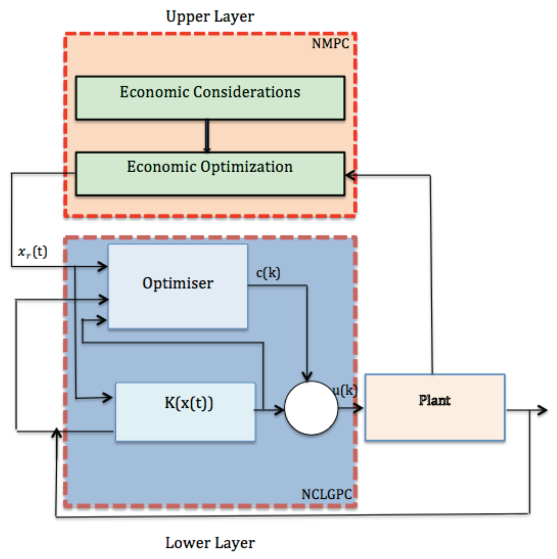
4. Controller Design

The control strategy proposed in this paper is described schematically in Figure 1. In the upper layer, the control is achieved by using an economic NMPC, while the lower layer uses a NCLGPC that combines an unconstrained nonlinear economic feedback control law $F\left(k\right)$ with the parameterization $c\left(k\right)$ associated with the closed-loop paradigm that allows the process constraints to be taken into account, thus improving the performance of the controller.

4.1. Upper Layer Problem Formulation

This layer provides the references $x_r$ for the lower layer by solving the following economic NMPC optimization:

$$\begin{array}{cc}\hfill \underset{u_r}{min}& {\int }_{t_k}^{t_{k+Ne}}{f}_{eco}({\tilde{x}}_r\left(\tau \right),u_r\left(\tau \right),\tau )d\tau \hfill \\ \hfill & \mathrm{subject}\mathrm{to}:\hfill \\ \hfill & {\dot{\tilde{x}}}_r\left(t\right)=A\left(t\right){\tilde{x}}_r\left(t\right)+\psi ({\tilde{x}}_r\left(t\right),u_r\left(t\right),0),\hfill \\ \hfill & {\tilde{x}}_r\left(t\right)=x\left(t\right),\hfill \\ \hfill & u_r\left(t\right)\in U,\hfill \\ \hfill & |{\dot{\tilde{x}}}_r\left(t\right)|⩽{\gamma }_r,\forall t\in [t_k,t_{k+Ne}[,\hfill \\ \hfill & {\tilde{x}}_r\left(t\right)\in \Omega \hfill \end{array}$$

(6)

where $N_e$ is the prediction horizon, $f_{eco}({\tilde{x}}_r\left(\tau \right),u_r\left(\tau \right),\tau )$ is the time-dependent economic cost function, ${\tilde{x}}_r\left(t\right)$ is the predicted trajectory of the system with the manipulated input $u_r\left(t\right)$ computed by the economic NMPC, and $x\left(t\right)$ is the state measurement obtained at time $t_k$.

In (6), the first constraint corresponds to the nominal model of the system, used to predict the future evolution of the states. The second constraint defines the initial condition of the optimization, which is the measurement of the state at instant $t_k$. The third constraint presents the control limitation of all manipulated inputs. The fourth constraint limits the rate of change of the state trajectory. The fifth constraint ensures that the economically optimal state trajectory is maintained in the domain $\Omega$. The last two constraints of the optimization problem of Equation (6) are used to guarantee closed-loop stability under this integrated framework and to ensure that the lower layer can force the system to track the state trajectory. This is a departure from other types of two-layer dynamic economic optimization architectures such as dynamic real-time optimization. The constraint on the rate of change of the economically optimal trajectory does pose a restriction on the feasible set of the optimization problem of Equation (6) and, thus, can affect the closed-loop economic performance of the control framework. However, a system that requires a large rate of change on the trajectory to achieve closed-loop economic performance that is better than steady-state may be undesirable for many applications based on practical considerations such as excessive strain on control actuators as well as the difficulty of forcing the system to track a rapidly changing operating trajectory in the presence of disturbances.

The gradient of the economic objective function is included in the cost function of the controller. Optimal conditions of the process at steady state are searched through the use of a rigorous nonlinear process model. The main advantage of the proposed strategy is that the resulting control/optimization problem can still be solved with a quadratic programming routine at each sampling step. The approach proposed may be comparable to the strategy that solves the full economic optimization problem inside the MPC controller where the resulting control problem becomes a nonlinear programming problem with a much higher computer load.

In general, the function $f_{eco}({\tilde{x}}_r\left(\tau \right),u_r\left(\tau \right),0)$ is not a quadratic function of the decision variables of the stated optimization problem. Consequently, the problem becomes a nonlinear programming problem, which may be difficult to solve. To overcome this problem, the function $f_{eco}$ is approximated by its gradient, as in [9], as follows. Suppose that the stationary prediction of the controller output related to the current input $u_r$ is ${\widehat{y}}_r$. Furthermore, consider that the economic function associated with the operation of the system is a concave function, whose maximum has to be searched and which can be represented as a function of the predicted state [10] as follows:

$$F=f_{eco}(u_r,{\widehat{y}}_r)$$

(7)

Then, assuming that the vector of the control action changes to $u_r+\delta u_r$, the first-order approximation of the gradient of the economic function is:

$${\xi }_{u_r+\delta u_r}=D+G\delta {\overline{u}}_r$$

(8)

where the calculations of D and G are detailed in [10], and $\delta {\overline{u}}_r=u_r\left(t_{k+N_e-1}\right)-u_r\left(t_{k-1}\right)$ is the total move of the input vector, D is the gradient vector at the present time and G is the Hessian of the economic function with respect to the inputs. The gradient vector ${\xi }_{u_r+\delta u_r}$ can be considered as a deviation vector in relation to the reference, which is equivalent to considering that the gradient of the economic function is zero at the optimum. As a result of these assumptions $f_{eco}$ can be approximated by a quadratic function as $f_{eco}={\xi }_{u+\delta u}^T{\xi }_{u_r+\delta u_r}$, so the optimization problem Equation (6) becomes:

$$\begin{array}{cc}\hfill \underset{u_r}{min}& {\int }_{t_k}^{t_{k+Ne}}{\xi }_{u_r\left(\tau \right)+\delta u_r\left(\tau \right)}^T{\xi }_{u_r\left(\tau \right)+\delta u_r\left(\tau \right)}d\tau \hfill \\ \hfill & \mathrm{subject}\mathrm{to}:\hfill \\ \hfill & {\dot{\tilde{x}}}_r\left(t\right)=A\left(t\right){\tilde{x}}_r\left(t\right)+\psi ({\tilde{x}}_r\left(t\right),u_r\left(t\right),0),\hfill \\ \hfill & {\tilde{x}}_r\left(t\right)=x\left(t\right),\hfill \\ \hfill & u_r\left(t\right)\in U,\hfill \\ \hfill & |{\dot{\tilde{x}}}_r\left(t\right)|⩽{\gamma }_r,\forall t\in [t_k,t_{k+Ne}[,\hfill \\ \hfill & {\tilde{x}}_r\left(t\right)\in \Omega \hfill \end{array}$$

(9)

4.2. Lower Layer Problem Formulation

At the lower process control level, we use a nonlinear closed-loop GPC (NCLGPC) to force the process state to track the trajectory $x_r^{*}\left(t\right)$ obtained by recursively solving the nominal model of Equation (1) with the manipulated input $u_r^{*}\left(t\right)$ applied for $t\in [t_k,t_k+t^{\prime }+N\Delta [$, where $t_k$ is the beginning of the operating period, $t^{\prime }$ is the operating period, and N is the prediction horizon of the NCLGPC. We assume that the NCLGPC synchronously recomputes the new manipulated inputs every $\Delta$ and $j=0,1,\cdots ,t^{\prime }/\Delta$. We define the system of Equation (1) in terms of the deviation from the economically optimal state trajectory $e\left(t\right)=x\left(t\right)-x_r^{*}\left(t\right)$,

The NCLGPC at $t_j$ is then formulated as follows:

$$\begin{array}{ll}\hfill \underset{c}{min}& {\int }_{t_j}^{t_{j+N}}\left(\right|\tilde{e}{\left(\tau \right)|}_Q+|u\left(\tau \right)-u_r^{*}\left(\tau \right){|}_R)d\tau \hfill \\ \hfill & \mathrm{subject}\mathrm{to}:\hfill \\ \hfill & \dot{\tilde{e}}\left(t\right)=A\left(t\right)\tilde{e}\left(t\right)+\psi (x\left(t\right),u\left(t\right),w\left(t\right))-\psi (x_r^{*}\left(t\right),u_r^{*}\left(t\right),0),\hfill \\ \hfill & u\left(t\right)=K\left(t\right)x\left(t\right)+c\left(t\right),\hfill \\ \hfill & u\left(t\right)\in U,\hfill \\ \hfill & e\left(t\right)=x\left(t\right)-x_r^{*}\left(t\right)\hfill \end{array}$$

(10)

where N is the prediction horizon of NCLGPC, $\tilde{e}\left(t\right)$ is the predicted deviation between the state trajectory predicted by the model Equation (1) with the manipulated input $u\left(t\right)$, and the economically optimal state trajectory $x_r^{*}\left(t\right)$. The optimal solution of the optimization Equation (10) is denoted by $u^{*}\left(t\right)$, defined for $t\in [t_j,t_{j+N}[$.

The controller in the lower layer is a NCLGPC based on an unconstrained nonlinear GPC, as an efficient advanced control technique for improving the operation of nonlinear plants. It is well known that closed-loop predictive control procedure is an effective strategy and has been exploited to decrease computational demand for solving optimization control problems. Traditionally, in this type of control, two modes of operation are considered over an infinite prediction horizon at each sampling time, this being a reformulation of a classical dual mode predictive control [9,18,19,20,21]. The predicted control moves are centered around an unconstrained stabilizing control law, $u\left(k\right)=K\left(x\right(k\left)\right)$ as computed in the Appendix A, over the whole prediction horizon, but some additive degrees of freedom, $u\left(k\right)=K\left(x\right(k\left)\right)+c\left(k\right)$ are added over a finite horizon to handle constraints and guarantee the feasibility of improving performance. Therefore there is an implicit switching between one mode of operation and the other as the process converges to the desired state.

In the optimization problem of Equation (10), the first constraint is the nominal deviation system of Equation (5). The second and third constraints define the structure of the closed-loop controller, where $K\left(t\right)$ is the terminal control law and the limitations of the manipulated variables $u\left(t\right)$, respectively. The last constraint presents the initial condition of the optimization of Equation (10).

The terminal region is obtained offline; here, the terminal control law $K\left(t\right)$ is calculated (Appendix A) in each iteration as in [9].

The implementation strategy of the proposed two-layer dynamic optimization can be summarized as follows:

• At time $t_k$ the upper layer economic NMPC with a prediction horizon $N_e$ receives the system state $x\left(t_k\right)$ from the process.
• The controller of Equation (6) computes the economically optimal state trajectory $x_r^{*}\left(t\right)$.
• The terminal control law $K\left(t\right)$ is computed.
• The solution of the optimization of Equation (9) denoted by $u^{*}\left(t\right)=K\left(t\right)x\left(t\right)+c^{*}\left(t\right)$ is calculated to track the economic state trajectory computed in step 2.
• Go to step 1, $t_k=t_{k+t^{\prime }}$

5. Stability

5.1. Definitions and Assumptions

We need to make certain definitions and assumptions about the system of Equation (5) to guarantee that the time-varying trajectory $x_r\left(t\right)$ can be tracked. We assume that the nominal system of Equation (1) is stabilizable at each fixed $x_r\in \Omega$.

The scalar comparison functions, $\mathcal{K}$, ${\mathcal{K}}_{\infty }$ and $\mathcal{KL}$, used to characterize the stability properties of a nonlinear systems are now recalled [22].

Definition 1.

A function $\alpha :[0,a[\to [0,\infty [$ is:

• a $\mathcal{K}$-function if it is continuous, strictly increasing and $\alpha \left(0\right)=0$.
• a ${\mathcal{K}}_{\infty }$-function if it is a $\mathcal{K}$-function and $a=\infty$ and $\alpha \left(r\right)\to \infty$ as $r\to \infty$.

Definition 2.

A function $\beta :[0,a[\times [0,\infty [\to [0,\infty [$ is a $\mathcal{KL}$-function if:

• for each fixed $t⩾0$, the function $\beta (r,t)$ is a $\mathcal{K}$-function, and
• for each fixed r, the mapping $\beta (r,t)$ is decreasing with respect to t and $\beta (r,t)\to 0$ as $t\to \infty$.

To be of practical interest, the stability conditions should not require Equation (1) so be solved explicitly. The direct method of Lyapunov is used, as it allows the stability properties of an equilibrium point from Equation (5) and its relationship with a positive-definite function $V\left(e\right)$ to be determined.

Definition 3.

Let $\mathbb{G}\subset {\mathbb{R}}^n$ be a nonempty open set. Let a function $f:\mathbb{G}\to \mathbb{R}$ have, at each point of the set $\mathbb{G}$, all partial derivatives continuous (i.e., function $x\to \frac{\partial f}{\partial x_j}\left(x\right)$ are continuous on $\mathbb{G}$ for each $j\in \{1,...,n\}$). Then we say that f is of the class ${\mathcal{C}}^1$ on $\mathbb{G}$. The set of all these functions is denoted by ${\mathcal{C}}^1\left(\mathbb{G}\right)$.

Definition 4.

Consider a function $V\in {\mathcal{C}}^1:{\Re }^n\to \Re$ that is positive-definite if $V\left(0\right)=0$ and $V\left(e\right)>0$ for all $e\ne 0$. Moreover, if $V\left(e\right)\to \infty$ as $\left|\right|e\left|\right|\to \infty$, then V is said to be radially unbounded.

Definition 5.

A bounded input $u:{\mathbb{R}}^{+}\to {\mathbb{R}}^m$ is called regularly persistent if

$\exists T>0;\exists T_0⩾0;\forall t>t_0,G(u,t,t+T)⩾0$ or equivalently, ${\lambda }_{min}\left(G(u,t,t+T)\right)⩾0$ (where ${\lambda }_{min}\left(G(u,t,t+T)\right)$ stands for the smallest eigenvalue of the Grammian G.

Assumption 1.

(Weak Controllability): There exists a $K_{\infty }$ function $\gamma (.)$ [23] such that, for every $x\in \Omega$, there exists $\mathit{u}$ such that $(x,\mathit{u})\in \mathbb{Z}$ and

$$\sum _{k=0}^{N-1}|u_k-u_r|⩽\gamma (|x-x_r|).$$

(11)

where $\mathbb{Z}$ is the set of admissible states. Assumption 1 is weaker than a controllability assumption, but it bounds the cost of steering an initial state x to $x_r$. It confines attention to those initial states that can be steered to $x_r$ in N steps, while satisfying the control and state constraints.

5.2. Stability Analysis

In this section, we present the stability properties of the proposed two-layer control framework presented in Equations (9) and (10). The following theorem provides sufficient conditions such that the NLCGPC can track the economically time varying trajectory $x_r^{*}\left(t\right)$.

Theorem 1.

The system of Equation (1) is exponentially stable under the optimizations of Equation (9) and Equation (10) if there exist ${\beta }_1>0$, ${\beta }_2>0$, $\gamma >0$, $L_u>0$, $L_e>0$, $L_w>0$ and matrices $P>0$ and $Q⩾0$ such that

$${\lambda }_{max}\left(Q\right)>2{\beta }_2(L_e+L_u\gamma )$$

(12)

Then,

$$\left|\right|e\left(t\right)\left|\right|⩽\frac{\sqrt{{\beta }_2}}{\sqrt{{\beta }_1}}{e}^{\frac{1}{2}{\alpha }_1\delta t}\left|\right|e\left(0\right)\left|\right|$$

(13)

where ${\lambda }_{max}$ stands for the biggest eigenvalue and ${\alpha }_1$ is:

$$\begin{array}{cc}\hfill {\alpha }_1& =\frac{2{\beta }_2(L_e+L_u\gamma )-{\lambda }_{max}\left(Q\right)}{{\beta }_1}\hfill \end{array}$$

The proof of this theorem requires the following Lemmas.

Lemma 1

([24]). Let u be a regularly persistent input for the system (1). Then, $\forall P\left(t\right)$ is a symmetric positive definite matrix, and there exist ${\beta }_1>0$ and ${\beta }_2>0$ such that

$$\forall t⩾0,{\beta }_1\mathcal{I}⩽P\left(t\right)⩽{\beta }_2\mathcal{I}$$

(14)

where $P\left(0\right)$ is an arbitrary symmetric definite matrix and $\mathcal{I}$ is the identity matrix with dimensions of $P\left(0\right)$.

Lemma 2

([25]). Let $v\left(t\right)$ be a positive differentiable function satisfying the inequality

$$\dot{v}\left(t\right)⩽f\left(t\right)v\left(t\right)+g\left(t\right)v^p\left(t\right),t\in I=[a,b],$$

(15)

where the functions $f\left(t\right)$ and $g\left(t\right)$ are continuous in I, and $p⩾0$, $p\ne 1$, is a constant. Then

$$\begin{array}{cc}\hfill v\left(t\right)⩽& exp\left({\int }_a^{t}f\left(s\right)ds\right)\hfill \\ \hfill & \times {\left[v^q\left(a\right)+q{\int }_a^{t}g\left(s\right)exp\left(-q{\int }_a^{s}f\left(\tau \right)d\tau \right)ds\right]}^{\frac{1}{q}}\hfill \end{array}$$

(16)

where $q=1-p$.

Proof of Theorem 1.

We define a Lyapunov function $V\left(t\right)$ that verifies the conditions of Definitions 3:

$$V\left(t\right)=e^T\left(t\right)P\left(t\right)e\left(t\right)$$

(17)

where the matrix $P\left(t\right)$ is the solution of the following Riccati equation:

$$A^T\left(t\right)P\left(t\right)+P\left(t\right)A\left(t\right)+\dot{P}\left(t\right)=-Q\left(t\right)$$

(18)

For $t\in [t_k,t_{k+1}]$

$$\begin{array}{cc}\hfill \dot{V}\left(t\right)& =2e^T\left(t\right)P\left(t\right)\dot{e}\left(t\right)+e^T\left(t\right)\dot{P}e\left(t\right)\hfill \\ \hfill & =2e^T\left(t\right)P\left(t\right)[A\left(t\right)e\left(t\right)+\psi (x\left(t\right),u^{*}\left(t\right),w\left(t\right))-\psi (x_r^{*}\left(t\right),u_r^{*}\left(t\right),0)]\hfill \\ \hfill & +e^T\left(t\right)\dot{P}\left(t\right)e\left(t\right)\hfill \end{array}$$

(19)

Using Equation (19) gives

$$\begin{array}{cc}\hfill \dot{V}\left(t\right)& =2e^T\left(t\right)P\left(t\right)\dot{e}\left(t\right)+e^T\left(t\right)\dot{P}e\left(t\right)\hfill \\ \hfill & =2e^T\left(t\right)P\left(t\right)[A\left(t\right)e\left(t\right)+\psi (x\left(t\right),u^{*}\left(t\right),w\left(t\right))-\psi (x_r^{*}\left(t\right),u_r^{*}\left(t\right),0)]\hfill \\ \hfill & +e^T\left(t\right)[-A^T\left(t\right)P\left(t\right)-P\left(t\right)A\left(t\right)-Q\left(t\right)]e\left(t\right)\hfill \\ \hfill & =-e^T\left(t\right)Q\left(t\right)e\left(t\right)+2e^T\left(t\right)P\left(t\right)[\psi (x\left(t\right),u^{*}\left(t\right),w\left(t\right))-\psi (x_r^{*}\left(t\right),u_r^{*}\left(t\right),0)]\hfill \\ \hfill & +e^T\left(t\right)P\left(t\right)A\left(t\right)e\left(t\right)-e^T\left(t\right)A^T\left(t\right)P\left(t\right)e\left(t\right)\hfill \\ \hfill & ⩽-{\lambda }_{max}{\left(Q\left(t\right)\right)\left|\right|e\left(t\right)\left|\right|}^2+{\lambda }_{min}{\left(P\left(t\right)A\left(t\right)\right)\left|\right|e\left(t\right)\left|\right|}^2-{\lambda }_{min}\left(A^T\left(t\right)P\left(t\right)\right){\left|\right|e\left(t\right)\left|\right|}^2\hfill \\ \hfill & +2\left|\right|e\left(t\right)\left|\right|.\left|\right|P\left(t\right)\left|\right|\times \left|\right|\psi (x\left(t\right),u^{*}\left(t\right),w\left(t\right))-\psi (x_r^{*}\left(t\right),u_r^{*}\left(t\right),0)\left|\right|\hfill \end{array}$$

(20)

By the Lipschitz property assumed for the vector $\psi$ and by Assumption 1, there exist positive constants $L_w$, $L_u$ and $L_e$ such that

$$\begin{array}{cc}\hfill & \left|\right|\psi (x\left(t\right),u^{*}\left(t\right),w\left(t\right))-\psi (x_r^{*}\left(t\right),u_r^{*}\left(t\right),0)\left|\right|\hfill \\ \hfill & ⩽L_e|x\left(t\right)-x_r^{*}\left(t\right)|+L_u|u^{*}\left(t\right)-u_r^{*}\left(t\right)|+L_w\left|w\left(t\right)\right|\hfill \\ \hfill & ⩽L_e\left|e\left(t\right)\right|+L_u\gamma \left|e\left(t\right)\right|+L_w\theta \hfill \end{array}$$

(21)

Substituting Equation (21) in Equation (20) and using Lemma 1, the derivative of the Lyapunov function becomes

$$\dot{V}\left(t\right)⩽[2{\beta }_2(L_e+L_u\gamma )-{\lambda }_{max}\left(Q\left(t\right)\right)]\left|\right|e\left(t\right){\left|\right|}^2+2{\beta }_2{L}_w\theta \left|\right|e\left(t\right)\left|\right|$$

(22)

and by Lemma 1

$${\beta }_1{\left|\right|e\left(t\right)\left|\right|}^2⩽e^T\left(t\right)P\left(t\right)e\left(t\right)⩽{\beta }_2{\left|\right|e\left(t\right)\left|\right|}^2$$

(23)

$$\begin{array}{cc}\hfill {\left|\right|e\left(t\right)\left|\right|}^2& ⩽\frac{V\left(t\right)}{{\beta }_1}⩽\frac{{\beta }_2}{{\beta }_1}{\left|\right|e\left(t\right)\left|\right|}^2\hfill \\ \hfill \left|\right|e\left(t\right)\left|\right|& ⩽\frac{\sqrt{V\left(t\right)}}{\sqrt{{\beta }_1}}⩽\frac{\sqrt{{\beta }_2}}{\sqrt{{\beta }_1}}\left|\right|e\left(t\right)\left|\right|\hfill \end{array}$$

(24)

Equation (22) becomes

$$\dot{V}\left(t\right)⩽{\alpha }_{1}V\left(t\right)+{\alpha }_2\sqrt{V\left(t\right)}$$

(25)

where

$${\alpha }_2=\frac{2{\beta }_2{L}_w\theta }{\sqrt{{\beta }_1}}$$

By Lemma 2, with

$$\begin{array}{cc}\hfill f\left(t\right)& ={\alpha }_1,g\left(t\right)={\alpha }_2\hfill \\ \hfill p& =\frac{1}{2},I=[t_k,t_{k+1}]\hfill \end{array}$$

Gives

$$V(t)⩽exp({\int }_{t_k}^t{\alpha }_{1}ds){[\sqrt{V(t_k)}-\frac{1}{2}{\int }_{t_k}^t{\alpha }_{2}exp(-\frac{1}{2}{\int }_{t_k}^s{\alpha }_1)ds]}^{\frac{1}{q}}$$

Replacing q by its value:

$$V(t)⩽exp({\int }_{t_k}^t{\alpha }_{1}ds){[\sqrt{V(t_k)}-\frac{1}{2}{\int }_{t_k}^t{\alpha }_{2}exp(-\frac{1}{2}{\int }_{t_k}^s{\alpha }_1)ds]}^2$$

That gives:

$$V{(t)}^{\frac{1}{2}}⩽{(exp({\int }_{t_k}^t{\alpha }_{1}ds))}^{\frac{1}{2}}[\sqrt{V(t_k)}-\frac{1}{2}{\int }_{t_k}^t{\alpha }_{2}exp(-\frac{1}{2}{\int }_{t_k}^s{\alpha }_1)ds]$$

That gives

$$\sqrt{V(t)}⩽exp(\frac{1}{2}{\alpha }_1(t-t_k))[\sqrt{V(t_k)}-\frac{{\alpha }_2}{{\alpha }_1}(1-exp(-\frac{1}{2}{\alpha }_1(t-t_k)))]$$

(26)

and we have:

$$0⩽exp(-\frac{1}{2}{\alpha }_1(t-t_k))$$

$$1-exp(-\frac{1}{2}{\alpha }_1(t-t_k))⩽1$$

$$\frac{{\alpha }_2}{{\alpha }_1}(1-exp(-\frac{1}{2}{\alpha }_1(t-t_k)))⩽\frac{{\alpha }_2}{{\alpha }_1}$$

$$-\frac{{\alpha }_2}{{\alpha }_1}⩽-\frac{{\alpha }_2}{{\alpha }_1}(1-exp(-\frac{1}{2}{\alpha }_1(t-t_k)))$$

$$\sqrt{V(t_k)}-\frac{{\alpha }_2}{{\alpha }_1}⩽\sqrt{V(t_k)}-\frac{{\alpha }_2}{{\alpha }_1}(1-exp(-\frac{1}{2}{\alpha }_1(t-t_k)))⩽\sqrt{V(t_k)}$$

Equation (26) becomes

$$\sqrt{V(t)}⩽exp(\frac{1}{2}{\alpha }_1(t-t_k))\sqrt{V(t_k)}$$

(27)

Following the same reasoning in the Appendix B, we obtain

$$\sqrt{V(t)}⩽exp(\frac{1}{2}{\alpha }_1\delta t)\sqrt{V(0)}$$

(28)

Using the second inequality of Equation (24), hence

$$\left|\right|e(t)\left|\right|⩽\frac{\sqrt{{\beta }_2}}{\sqrt{{\beta }_1}}exp(\frac{1}{2}{\alpha }_1\delta t)\left|\right|e(0)\left|\right|$$

(29)

Consequently, the error between the actual system trajectory and the economically optimal trajectory $e\left(t\right)=x\left(t\right)-x_r\left(t\right)$ is bounded by:

$$\underset{t\to \infty }{lim}\left|\right|e\left(t\right)\left|\right|=0.$$

(30)

6. Application to WWTP

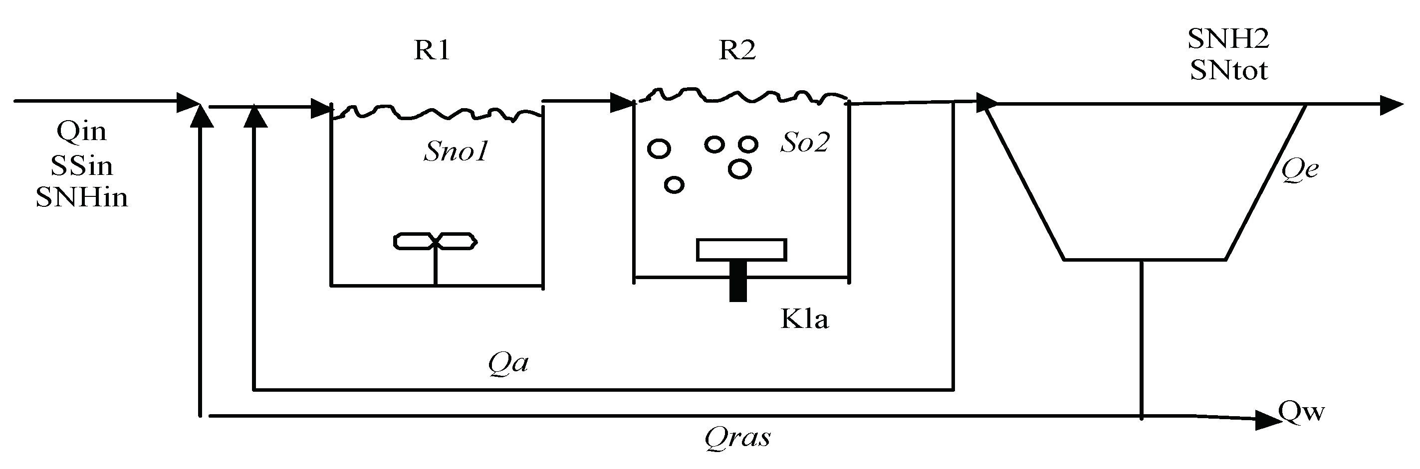
WWTPs are large nonlinear systems characterized by the complexity of the biological and biochemical phenomena involved. The nonlinear dynamics of the system, the large range of time constants (from a few minutes to several days) observed in the different biological processes and the significant perturbations in the flow and load of the influent make WWTPs a really challenging case study from the control point of view. WWTPs have to be operated efficiently, minimizing the energy and consumption of resources, while meeting strict environmental regulations. Therefore, the advanced control strategies proposed in this paper are a promising alternative for improving their performance and economics.

6.1. Process Model

The WWTP process selected as a case study follows the specifications given in the Benchmark Simulation Protocol (BSM1) [26] which are widely accepted by the scientific community. However, the model focuses on the N-Removal process. The Benchmark Simulation Model (BSM1) has been widely applied to test control strategies for the Activated Sludge Process (ASP) in wastewater treatment plants. It consists of 5 bioreactors: 2 anoxic and 3 aerobic. In the simplified model considered in this work, only the significant variables of the BSM1 model on a medium time scale are taken into account. The processes with slow variations in time (the growth of autotrophic and heterotrophic microorganisms and hydrolyze processes) are neglected. The BSM1 representation is reduced to one anoxic and one aerated reactor as shown in Figure 2. The volumes of the two tanks are 2000 m${}^3$ and 3999 m${}^3$, to make them equivalent to total volumes of the anoxic and the aerobic compartments in the BSM1.

The following equations represent the dynamic behavior of the plant.

• Anoxic reactor:

$$\begin{array}{cc}\hfill {\dot{S}}_{NH1}& =\frac{1}{V_1}\left[Q_{in}{S}_{NHin}+Q_a{S}_{NH2}-(Q_{in}+Q_a)S_{NH1}\right]-i_{xb}{\rho }_{11}-i_{xb}{\rho }_{21}\hfill \\ \hfill & -(i_{xb}+\frac{1}{Y_A}){\rho }_{31}\hfill \\ \hfill {\dot{S}}_{NO1}& =\frac{1}{V_1}\left[Q_a{S}_{NO2}-(Q_{in}+Q_a)S_{NO1}\right]-\frac{1-Y_H}{2.86Y_H}{\rho }_{21}+\frac{1}{Y_A}{\rho }_{31}\hfill \\ \hfill {\dot{S}}_{S1}& =\frac{1}{V_1}\left[Q_{in}{S}_{Sin}+Q_a{S}_{S2}-(Q_{in}+Q_a)S_{S1}\right]-\frac{1}{Y_H}{\rho }_{11}-\frac{1}{Y_H}{\rho }_{21}\hfill \\ \hfill {\dot{S}}_{O1}& =\frac{1}{V_1}\left[Q_a{S}_{O2}-(Q_{in}+Q_a)S_{O1}\right]-\frac{1-Y_H}{Y_H}{\rho }_{11}-(\frac{4.57}{Y_A}+1){\rho }_{31}\hfill \end{array}$$

(31)

• Aerobic reactor:

$$\begin{array}{cc}\hfill {\dot{S}}_{NH2}& =\frac{1}{V_2}\left[(Q_{in}+Q_a)(S_{NH1}-S_{NH2})\right]-i_{xb}{\rho }_{12}-(i_{xb}+\frac{1}{Y_A}){\rho }_{32}\hfill \\ \hfill {\dot{S}}_{NO2}& =\frac{1}{V_2}\left[(Q_{in}+Q_a)(S_{NO1}-S_{NO2})\right]-\frac{1-Y_H}{2.86Y_A}{\rho }_{22}+\frac{1}{Y_A}{\rho }_{32}\hfill \\ \hfill {\dot{S}}_{S2}& =\frac{1}{V_2}\left[(Q_{in}+Q_a)(S_{S1}-S_{S2})\right]-\frac{1}{Y_H}{\rho }_{12}-\frac{1}{Y_H}{\rho }_{22}\hfill \\ \hfill {\dot{S}}_{O2}& =\frac{1}{V_2}\left[(Q_{in}+Q_a)(S_{O1}-S_{O2})\right]-\frac{1-Y_H}{Y_H}{\rho }_{12}-\frac{4.57-Y_A}{Y_A}{\rho }_{32}\hfill \\ \hfill & +KLa(S_{O,Sat}-S_{O2})\hfill \end{array}$$

(32)

In the first reactor, the anoxic growth of heterotrophic biomass is the main biological process, related to denitrification:

$${\rho }_{21}={\mu }_H·(\frac{S_{S1}}{K_S+S_{S1}})·(\frac{K_{O,H}}{K_{O,H}+S_{O1}})·(\frac{S_{NO1}}{K_{NO}+S_{S1}}){\eta }_g{X}_{B,H}$$

(33)

In the second reactor, where there is a higher concentration of oxygen, the aerobic growths of heterotrophic and autotrophic biomass are considered, related to nitrification:

$$\begin{array}{cc}\hfill {\rho }_{12}& ={\mu }_H·(\frac{S_{S2}}{K_S+S_{S2}})·(\frac{S_{O2}}{K_{O,H}+S_{O2}})·X_{B,H}\hfill \\ \hfill {\rho }_{32}& ={\mu }_A·(\frac{S_{NH2}}{K_{NH}+S_{NH2}})·(\frac{S_{O2}}{K_{O,A}+S_{O2}})·X_{B,A}\hfill \end{array}$$

(34)

The rest of the processes $\rho$ are assumed to be zero in Equations (32) and (33).

The definitions of the state variables are given in

Table 1. List of state variables of the model.

Notation	Definition	Unit
$S_{NH}$	$N{H}_4+N{H}_3$ concentration	grN/m${}^3$
$S_{NO}$	Nitrate and nitrite concentration	grN/m${}^3$
$S_S$	Readily biodegradable substrate concentration	grCOD/m${}^3$
$S_O$	Dissolved oxygen concentration	gr/m${}^3$

. The definitions of the kinetic and physical parameters are presented in

Table 2. Process characteristics.

Notation	Definition
$Q_{in}$	Influent flow rate
$S_{S,in}$	Influent organic matter concentration
$S_{NH,in}$	Influent ammonium compounds concentration
$Q_a$	Internal recycle flow
$K_{La}$	Oxygen transfer coefficient
$V_1$	Anoxic reactor volume
$V_2$	Aerobic reactor volume

and

Table 3. Kinetic parameters and stoichiometric coefficient characteristics.

Notation	Definition
$S_{O,sat}$	Oxygen saturation concentration
${\mu }_H$	Heterotrophic max. specific growth rate
$K_S$	Half saturation coefficient for heterotrophs
$K_{O,H}$	Oxygen saturation coefficient for heterotrophs
$K_{NH}$	Ammonia saturation coefficient for heterotrophs
$K_{O,A}$	Oxygen saturation coefficient for autotrophs
$Y_H$	Heterotrophic yield
$Y_A$	Autotrophic yield
$i_{xb}$	Nitrogen fraction in biomass

, and their values are the same as for BSM1 [24].

6.2. Operating Conditions

The BSM1 defines the operational requirements of the plant as well as some performance criteria to characterize the effluent quality and the energy consumption [26]:

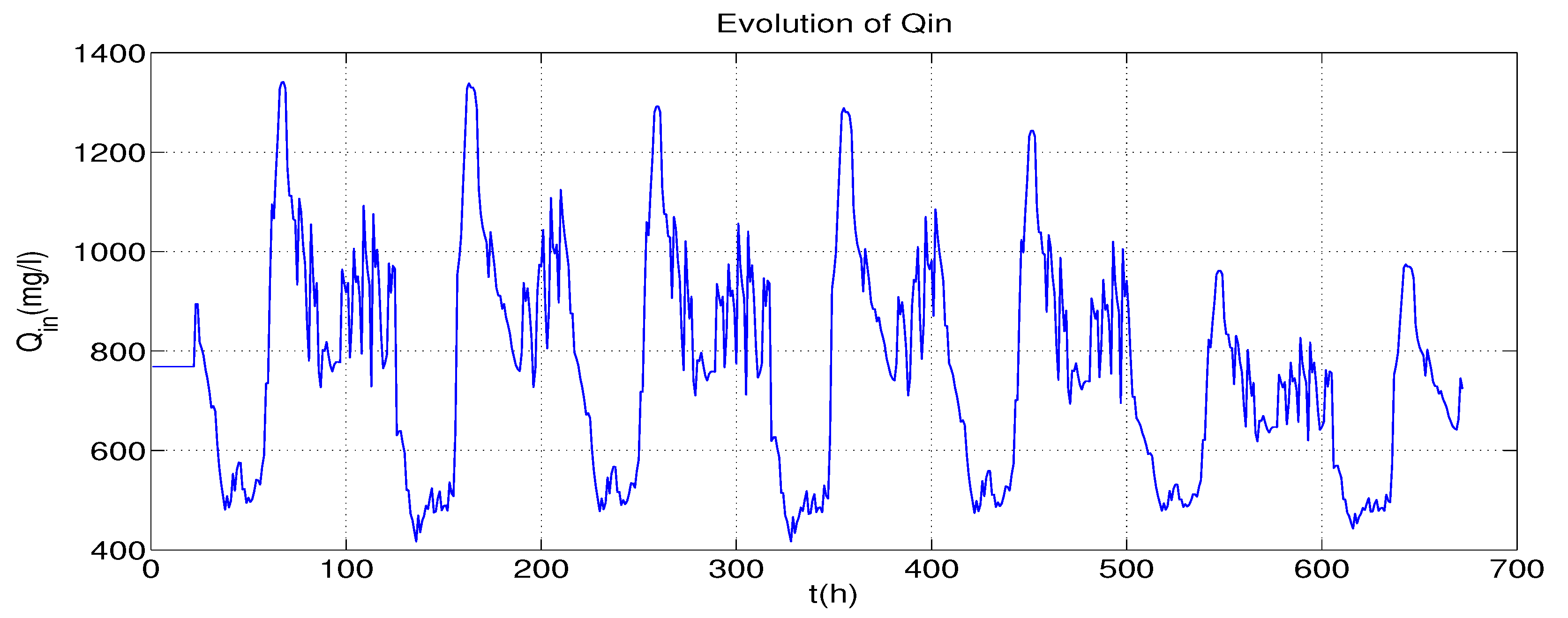
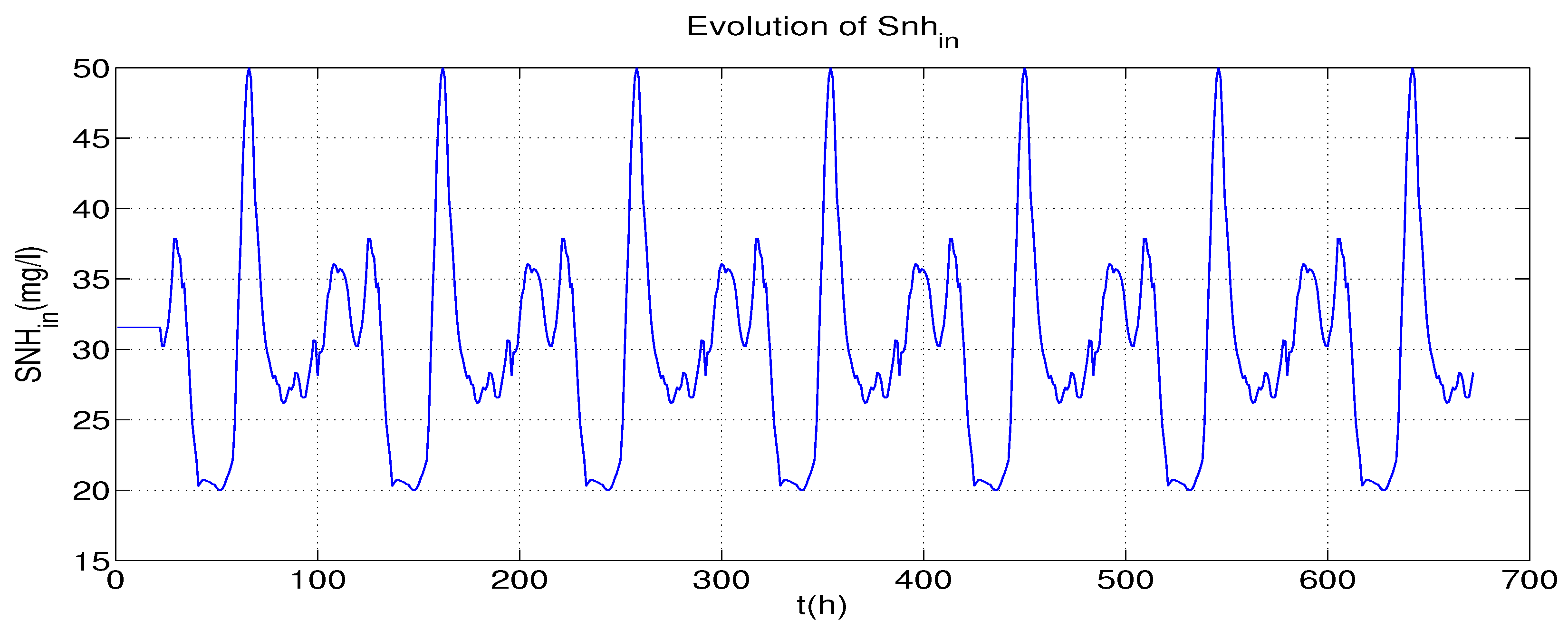
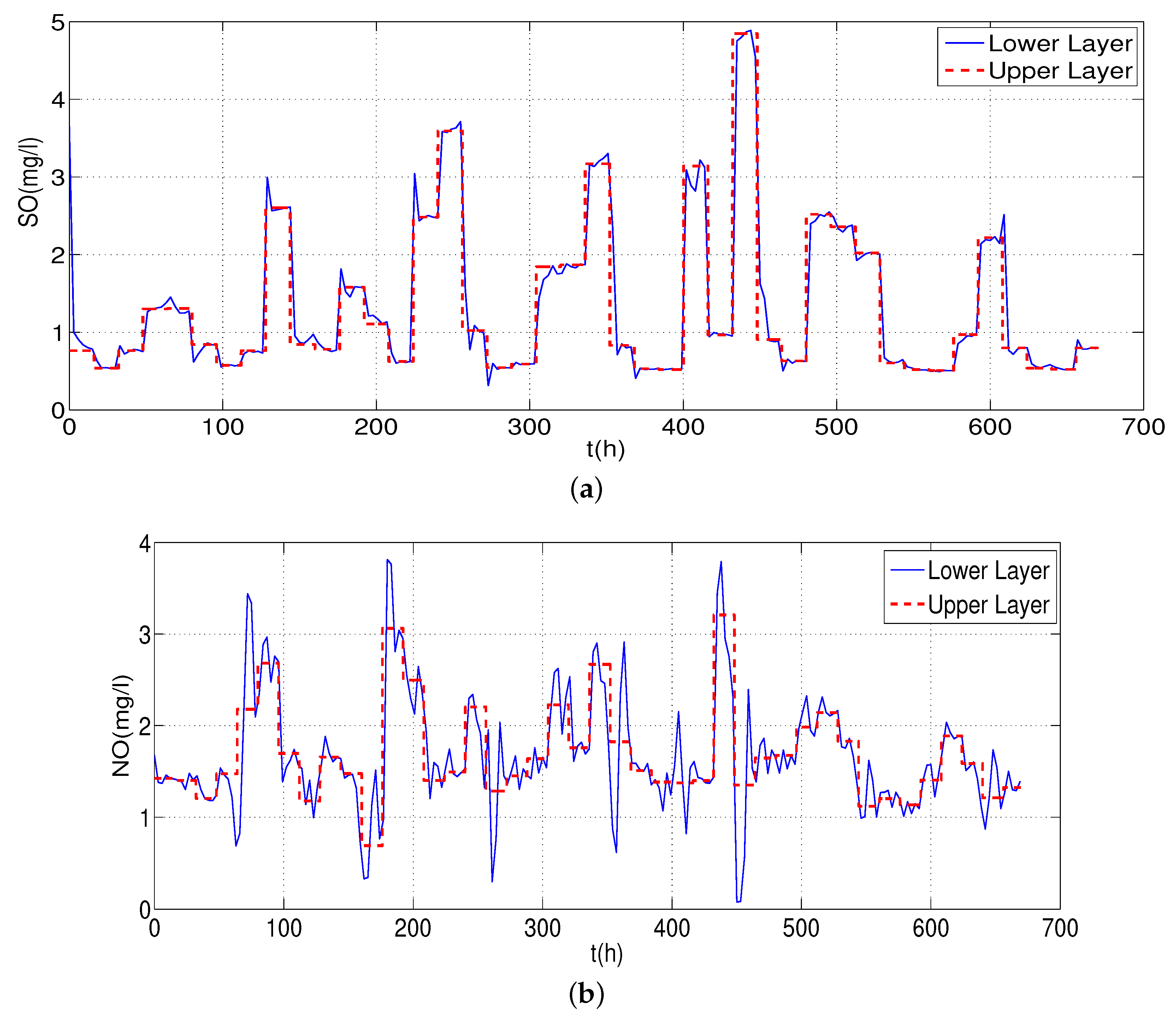
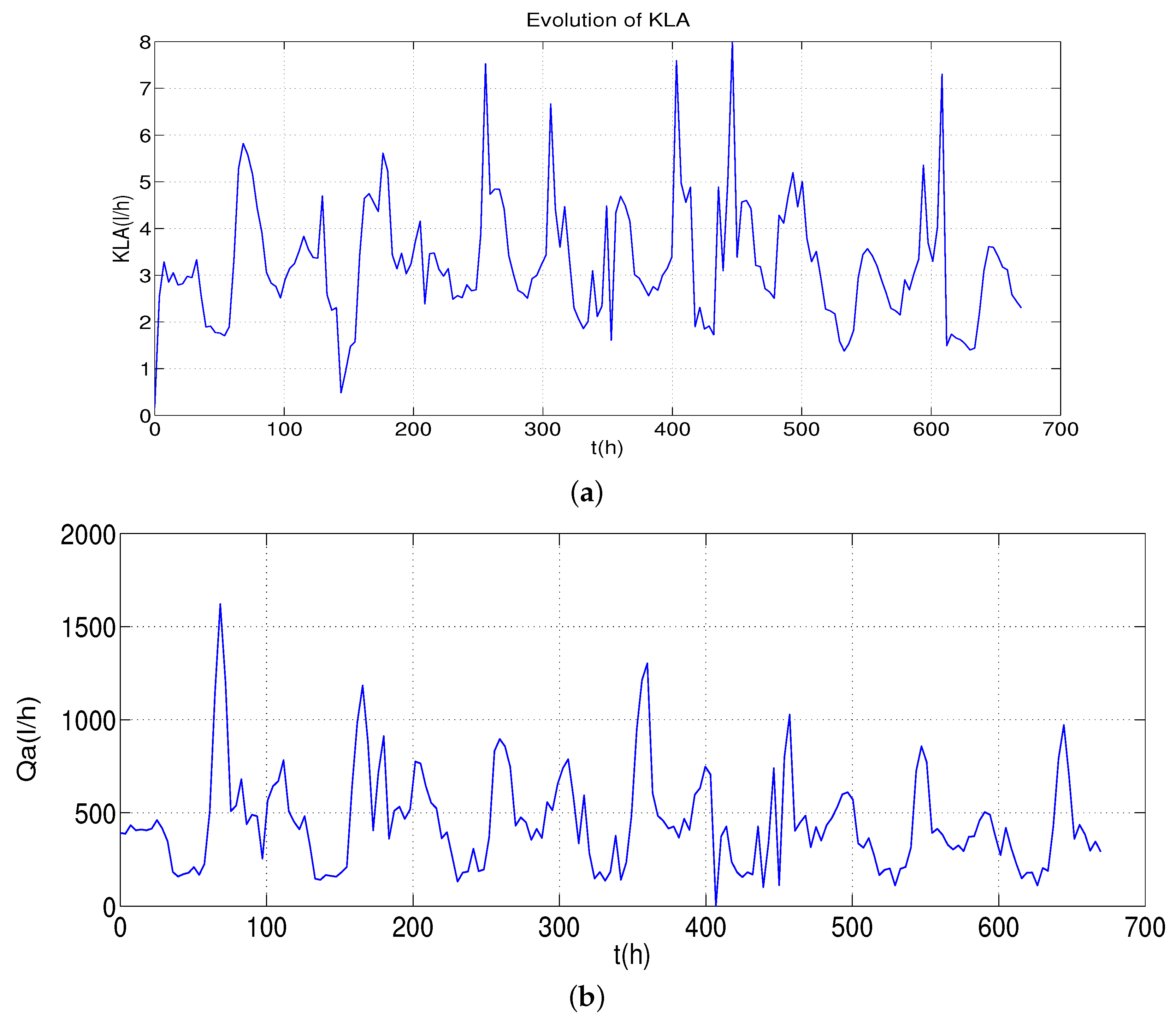
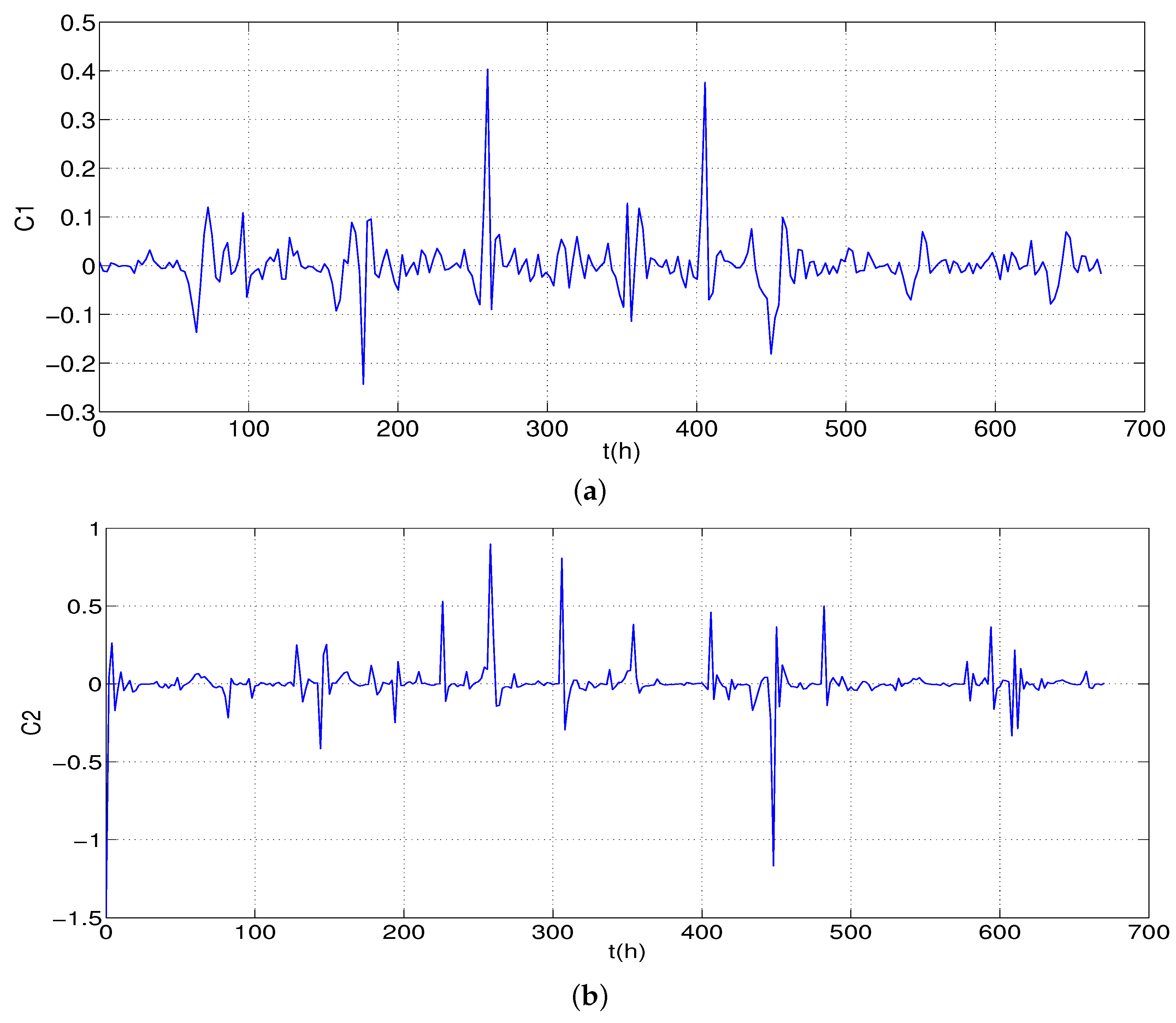
• Influent load and disturbances: In order to test the performance of the control strategy in different situations, the BSM1 provides standardized influent data considering different weather situations. In this work, data for 336 h, corresponding to 2 weeks starting at time 168 h, are considered, with a sampling period of 0.25 h (= 15 min). Figure 3, Figure 4 and Figure 5 present the profiles for stormy weather.
• Bounds: The limits on the effluent–ammonium $\left(S_{NH}\right)$ concentration, total nitrogen $\left(N_{tot}\right)$ concentration, suspended solid $\left(S_{S,e}\right)$ concentration, biological oxygen demand over a 5-day period $\left(BO{D}_5\right)$ and $\left(COD\right)$ are given in

  Table 4. Bounds of the effluent concentrations.

  Effluent Qualities	Upper Bound	Unit
  $S_{NH}$	4	mg/L
  $S_{NO}$	10	mg/L
  $N_{tot}$	18	mg/L
  $TSS$	30	mg/L
  $COD$	100	mg/L
  $K_{La}$	200	d${}^{-1}$
  $Q_a$	3850	m${}^3$/d

  .

6.3. Performance Indices

The measures used to characterize the effluent quality and energy usage during the N-removal process are the standard performance indices recommended in the BSM1 platform for the evaluation of control strategies applied to WWTPs.

In BSM1, the total average pumping energy (PE) over a certain period of time, T, depends directly on the internal recirculation flow rate $Q_a$, according to [24], calculated as:

$$PE=\frac{0.04}{T}{\int }_{t_0}^{t_0+T}(Q_a\left(t\right)+Q_w\left(t\right))dt$$

(35)

expressed in kWh/day. In $\left(36\right)$, $Q_a$ denotes the return sludge flow rate and $Q_w$ the excess sludge flow rate, both in units of m${}^3$/day.

The aeration energy (AE) in kWh/day required to aerate the last three compartments is written as:

$$AE=\frac{24}{T}{\int }_{t_0}^{t_0+T}\sum _{i=3}^5(0.4032KL{a}_i{\left(t\right)}^2+7.8408KL{a}_i\left(t\right))dt$$

(36)

where $KL{a}_i\left(t\right)$ is the oxygen transfer function in the aerated tank number i in units of $h^{-1}$.

The effluent quality (EQ) in Kg pollution/day is defined as a weighted daily average of the total concentration of different compounds in the effluent, as follows:

$$\begin{array}{cc}\hfill EQ& =\frac{1}{1000T}{\int }_{t_0}^{t_0+T}(2TS{S}_e\left(t\right)+CO{D}_e\left(t\right)+30N_{tot,e}\left(t\right)\hfill \\ \hfill & +10S_{NO}\left(t\right)+2BO{D}_e\left(t\right))Q_e\left(t\right)dt\hfill \end{array}$$

(37)

where:

$$\begin{array}{cc}\hfill CO{D}_e& =(S_{S,e}+X_{B,Ae}+X_{B,He})g/m^3\hfill \\ \hfill BO{D}_e& =0.25((1-0.08)+(1-0.08)(X_{B,A}+X_{B,H}))g/m^3\hfill \\ \hfill N_{tot,e}& =S_{NOe}+S_{NHe}+i_{xb}(X_{B,He}+X_{B,Ae})g/m^3\hfill \\ \hfill TS{S}_e& =0.75(X_{B,Ae}+X_{B,He})g/m^3\hfill \end{array}$$

(38)

In the above equation, TSS denotes total suspended solids and $N_{tote}$ is the total nitrogen concentration in the effluent. The subscript ‘$e$’ indicates that those concentrations are associated with the effluent of the settler. The weighting factors of $TS{S}_e$, $CO{D}_e$ and $N_{tote}$, and $BO{D}_e$ are adopted from [24]. The model considered in this work was developed assuming that the separation in the settler produces: $X_{B,Ae}=0.0038.X_{B,A}$ and $X_{B,He}=0.0038.X_{B,H}$.

The total cost expressed in $(EUR/day)$ can be calculated during the interval T by:

$$OCI=w_3(AE+PE)$$

(39)

6.4. Control Problem Formulation

The paper has two major aims. The first one is to show the advantages of a two-layer structure compared with a single-layer and the second one is to provide a theoretical framework of the stability by proving that the deviation between the lower layer and the economically optimal closed-loop trajectory computed by the upper layer is bounded. Two advanced control strategies, both based on nonlinear model predictive control, are tested in the WWTP.

6.4.1. Two Layer

(I).

Lower layer control problem

In this work, the NCLGPC algorithm is applied in the lower layer to control the oxygen $S_{O2}$ in the aerobic reactor, and the nitrate levels $S_{NO1}$ in the anoxic reactor. This is carried by minimizing the cost function in $\left(10\right)$ subject to the corresponding constraints from Table 4. The manipulated variables are the oxygen transfer coefficient $KLa$ and the internal recycle flow rate $Q_a$, considering the influent flow $\left(Q_{in}\right)$ (Figure 3), the organic matter concentration $\left(S_{S,in}\right)$ (Figure 4) and the ammonium concentration $\left(S_{NH,in}\right)$ (Figure 5) in the influent are measurable disturbances.

Summarizing, the specific WWTP control problem variables considered in this application are:

• The state vector: $x\left(t\right)={\left[S_{NH1}{S}_{NO1}{S}_{S1}{S}_{O1}{S}_{NH2}{S}_{NO2}{S}_{S2}{S}_{O2}\right]}^T$.
• The output variables: $y\left(t\right)={\left[S_{NO1}{S}_{O2}\right]}^T$.
• The manipulated variables: $u\left(t\right)={\left[Q_{a}KLa\right]}^T$.
• The measured disturbances: $w\left(t\right)={\left[Q_{in}{S}_{S,in}{S}_{NH,in}\right]}^T$.

Rewriting the prediction model of Equations (32) and (33) as in Equation (1) gives:

$$\dot{x}\left(t\right)=A\left(t\right)x\left(t\right)+\psi (x\left(t\right),u\left(t\right),w\left(t\right))$$

(40)

where

$$A\left(t\right)=\left[\begin{array}{cccccccc}\frac{-Q_{in}}{V_1}& 0& 0& 0& 0& 0& 0& 0\\ 0& \frac{-Q_{in}}{V_1}& 0& 0& 0& 0& 0& 0\\ 0& 0& \frac{-Q_{in}}{V_1}& 0& 0& 0& 0& 0\\ 0& 0& 0& \frac{-Q_{in}}{V_1}& 0& 0& 0& 0\\ \frac{Q_{in}}{V_2}& 0& 0& 0& \frac{-Q_{in}}{V_2}& 0& 0& 0\\ 0& \frac{Q_{in}}{V_2}& 0& 0& 0& \frac{-Q_{in}}{V_2}& 0& 0\\ 0& 0& \frac{Q_{in}}{V_2}& 0& 0& 0& \frac{-Q_{in}}{V_2}& 0\\ 0& 0& 0& \frac{Q_{in}}{V_2}& 0& 0& 0& \frac{-Q_{in}}{V_2}\end{array}\right]$$

Note that, for the WWTP, $Q_{in}$ is a positive slow time varying variable and, since $A\left(t\right)$ is a lower triangular matrix with negative diagonal entries, i.e., with negative eigenvalues $\forall t⩾0$, the assumed condition on $A\left(t\right)$ in the problem statement (Section 1) is verified.

$$\begin{gathered} \psi (x\left(t\right),u\left(t\right),w\left(t\right))= \\ \left[\begin{array}{c}\frac{1}{V_1}\left[Q_{in}{S}_{NHin}+Q_a{S}_{NH2}-Q_a{S}_{NH1}\right]-i_{xb}{\rho }_{11}-i_{xb}{\rho }_{21}-(i_{xb}+\frac{1}{Y_A}){\rho }_{31}\hfill \\ \frac{1}{V_1}\left[Q_a{S}_{NO2}-Q_a{S}_{NO1}\right]-\frac{1-Y_H}{2.86Y_H}{\rho }_{21}+\frac{1}{Y_A}{\rho }_{31}\hfill \\ \frac{1}{V_1}\left[Q_{in}{S}_{Sin}+Q_a{S}_{S2}-Q_a{S}_{S1}\right]-\frac{1}{Y_H}{\rho }_{11}-\frac{1}{Y_H}{\rho }_{21}\hfill \\ \frac{1}{V_1}\left[Q_a{S}_{O2}-Q_a{S}_{O1}\right]-\frac{1-Y_H}{Y_H}{\rho }_{11}-(\frac{4.57}{Y_A}+1){\rho }_{31}\hfill \\ \frac{1}{V_2}\left[Q_a(S_{NH1}-S_{NH2})\right]-i_{xb}{\rho }_{12}-(i_{xb}+\frac{1}{Y_A}){\rho }_{32}\hfill \\ \frac{1}{V_2}\left[Q_a(S_{NO1}-S_{NO2})\right]-\frac{1-Y_H}{2.86Y_A}{\rho }_{22}+\frac{1}{Y_A}{\rho }_{32}\hfill \\ \frac{1}{V_2}\left[Q_a(S_{S1}-S_{S2})\right]-\frac{1}{Y_H}{\rho }_{12}-\frac{1}{Y_H}{\rho }_{22}\hfill \\ \frac{1}{V_2}\left[Q_a(S_{O1}-S_{O2})\right]-\frac{1-Y_H}{Y_H}{\rho }_{12}-\frac{4.57-Y_A}{Y_A}{\rho }_{32}+KLa(S_{O,Sat}-S_{O2})\hfill \end{array}\right] \end{gathered}$$

(II).

Upper layer control problem

In the upper layer, the economic function to be minimized subject to the corresponding constraints from Table 4 is:

$$f_{eco}(Kla\left(t\right),Q_a\left(t\right))=w_3(AE\left(Kla\left(t\right)\right)+PE\left(Q_a\left(t\right)\right)$$

(41)

where $AE$ and $PE$ are defined in $\left(36\right)$ and $\left(37\right)$.

In order to defined the control problem in $\left(9\right)$, the gradient of $f_{eco}$ has been computed according to $\left(8\right)$, giving us:

$$D=\left[\begin{array}{cc}0.04& 0.8064KLa+0.4032\end{array}\right]$$

$$G=\left[\begin{array}{cc}0& 0\\ 0& 19.3536\end{array}\right]$$

6.4.2. One Layer

The one-layer optimization problem proposed in [9] consists of the optimization of a cost function that includes the penalization of control error, of control efforts and the same $\left(f_{eco}\right)$ for the economic objectives:

$$\begin{array}{cc}\hfill J=& \sum _{i=1}^{n_y}\left|\right|w_1\left(r(k+i|k)\right)-{y(k+i|k)\left|\right|}_2^2+\sum _{i=0}^{n_u-1}\left|\right|w_2\Delta u(k+i|k){\left|\right|}_2^2\hfill \\ \hfill +& \sum _{i=1}^{n_y}{w}_3{f}_{eco}(u(k+i|k),y(k+i|k))\hfill \end{array}$$

subject to the following constraints:

$$\begin{array}{cc}\hfill u_{min}& ⩽u(k+i|k)⩽u_{max},i=0,\cdots ,n_u-1\hfill \\ \hfill y_{min}& ⩽y(k+i|k)⩽y_{max},i=1,\cdots ,n_y\hfill \\ \hfill \Delta u_{min}& ⩽\Delta u(k+i|k)⩽\Delta u_{max},i=0,\cdots ,n_u-1\hfill \\ \hfill x(k+i|k)& =A\left(x\right(k+i\left|k\right)\left)x\right(k+i\left|k\right)+B\left(x\right(k+i\left|k\right)\left)u\right(k+i\left|k\right),k⩾1\hfill \\ \hfill y(k+i|k)& =C\left(x\right(k+i\left|k\right)\left)x\right(k+i\left|k\right),k⩾1\hfill \end{array}$$

Some specific characteristics of this control strategy are:

• The predicted control moves are centered around an unconstrained stabilizing control law, $u\left(k\right)=K\left(x\right(k\left)\right)x\left(k\right)$, over the whole prediction horizon, and some additive degrees of freedom, $c\left(k\right)$, are added over a finite horizon to handle constraints.
• In the objective function the nonlinear economic term is replaced by its gradient.
• The prediction model, a nonlinear phenomenological model of the plant, is written as a state dependent coefficient model, also called extended linearization.

7. Simulations Settings

The economic NMPC algorithm uses the phenomenological model of the plant described in Equations (32)–(35) for predictions. The fmincon method of Matlab, based on sequential quadratic programming, uses each sampling time to obtain the optimal manipulated variables.

After some preliminary tests, the selected values to tune the economic NMPC for the upper layer are the control horizon $m_e=2$, prediction horizon $N_e=4$ and the weight of the economic function is $w_3=1$, while the tuning parameters of the optimizing controller for the lower layer are control horizon $m=2$, prediction horizon $N=4$, output weight $w_1=diag(0.155,0.01,0.155,0.01)$ and input weight $w_2=diag(0.01,0.01)$.

Figure 3, Figure 4 and Figure 5 present the different profiles of perturbations of $BSM1$ used in this study. In this influent, we can observe strong variations in the flow and concentrations during dry weather.

The performance assessment is made at two levels. The first level concerns the control design. The second level measures the effect of the control strategy on plant performance.

8. Simulations Results

Several simulations are carried out to study the process behavior with the controller and their effect on process economics and removal efficiency. The performance indices provided by the BSM1 platform are used to evaluate the process performance, with the different controllers in the operating period under characteristic storm weather influent variations.

The evolution of the most relevant process variables along the operating horizon is presented in the following figures.

Figure 6a,b present the two outputs that are, respectively, the dissolved oxygen in the aerobic reactor and the nitrate in the anoxic reactor. From the Figure 6, the ability of the controller to track the desired set point and disturbances rejection can be appreciated. Figure 7a,b present the evolution of the concentrations $SN{H}_2$ and $N-Total$. Good tracking of the controller is observed in spite of the frequent changes of set point and the strong variations in the influent. It is observed that the concentrations SNH2 and SNtot are below the limits most of the simulation time.

The two manipulated variables are shown in Figure 8, indicating that suitable control signals, $K_{la}$ and $Q_a$, drive the process to follow the set point, while satisfying the constraints imposed. Finally, Figure 9 presents the evolution of the degree of freedom C.

The criteria for evaluating the advantages of the implementation of the different architectures are the tradeoff between economic benefit, process performance, and complexity of the control structure. The performance evaluation criteria is the indicated in the BSM1 protocol for WWTPs.

In order to compare the economic efficiency of the proposed strategy developed in this paper, the performance of the plant with a two layer structure is compared with a one layer nonlinear economic closed-loop generalized predictive control described in Section 6.4.2 (for more details about this controller, please see [9]). The comparison is done in terms of the overall cost index (Equation (40)), aeration energy (Equation (37)), pumping energy (Equation (36)) and effluent quality (Equation (38)). To make a fair comparison, the same process disturbances as in Figure 3, Figure 4 and Figure 5 were applied to each closed-loop system simulation. The details of the comparisons in stormy weather are shown in

Table 5. Comparison of performance indices for one-layer and two-layer strategies.

Strategy Index	One Layer [9]	Two Layers	%
$AE$	1449.40	1190.40	−17.87%
$PE$	421.55	401.64	−4.72%
$EQ$	5897.00	5845.00	−0.88%
$OCI$	1870.90	1592.10	−14.99%

.

Table 5 shows that the two-layer strategy improves the economic aspect by reducing the $OCI$ index by $14.99\%$, the $AE$ by $17.87\%$ and the $PE$ by $4.72\%$, which proves that the proposed two-layer controller is sufficient for good performance and, in addition, this control could be easily extended to other applications.

9. Conclusions

In this work, we have proposed a two-layer strategy for integrating dynamic economic optimization and nonlinear closed-loop GPCs for nonlinear systems. In the upper layer, an economic NMPC is used to compute an economically optimal time-varying operating trajectory. Instead of including the nonlinear economic cost in the objective function, an approximation of the reduced gradient of the economic function is used. The lower layer is used to compute feedback control actions that force the outputs of the process to track the trajectories received from the upper layer.The controller used in this layer is a nonlinear closed-loop GPC. Instead of the classic dual-mode MPC (model predictive controller) schemes, where the terminal control law defined in the terminal region is obtained offline by solving a linear quadratic regulator problem, here, the terminal control law is determined online by an unconstrained nonlinear generalized predictive control. We have proved that the deviation between the actual closed-loop system and the economically optimal closed-loop trajectory is bounded. This paper presents a two-level hierarchical control structure for biological wastewater treatment plants, with the goal of improving effluent quality and reducing operational costs. Modifying the tuning parameters of the higher level, a tuning region is determined in which the effluent quality and operational costs are simultaneously improved.

The proposed methodology has been successfully applied to the N-Removal process in a WWTP. The strategy drives the plant to the economically optimal operating condition in spite of strong disturbances in the influent. The application of the proposed control strategies reduces the operational costs by around 15%, together with a satisfactory compromise regarding effluent quality in comparison with the one-layer strategy. The methodology of this work is general and can easily be extended to other applications.

References

1. Edgar, T. Control and operations: When does controllability equal profitability? Comput. Chem. Eng. 2004, 29, 41–49. [Google Scholar] [CrossRef]
2. Darby, M.L.; Nikolau, M.; Jones, J.; Nicholson, D. RTO: An overview and assessment of current practice. J. Process Control 2011, 21, 874–884. [Google Scholar] [CrossRef]
3. Rawlings, J.B.; Patel, N.R.; Risbeck, M.J.; Maravelias, C.T.; Wenzel, M.J.; Turney, R.D. Economic MPC and real-time decision making with application to large-scale HVAC energy systems. Comput. Chem. Eng. 2018, 114, 89–98. [Google Scholar] [CrossRef]
4. Revollar, S.; Vega, P.; Vilanova, R.; Francisco, M. Optimal Control of Wastewater Treatment Plants Using Economic-Oriented Model Predictive Dynamic Strategies. Appl. Sci. 2017, 7, 813. [Google Scholar] [CrossRef]
5. De Prada, C.; Sarabia, D.; Gutierrez, G.; Gomez, E.; Marmol, S.; Sola, M.; Pascual, C.; Gonzalez, R. Integration of RTO and MPC in the Hydrogen Network of a Petrol Refinery. Processes 2017, 5, 3. [Google Scholar] [CrossRef]
6. Rawlings, J.B.; Amrit, R. Optimizing Process Economic Performance Using Model Predictive Control. In Nonlinear Model Predictive Control; Magni, L., Raimondo, D.M., Allgöwer, F., Eds.; Lecture Notes in Control and Information Sciences; Springer: Berlin/Heidelberg, Germany, 2009; Volume 384. [Google Scholar]
7. Ellis, M.; Christofides, P.D. Integrating dynamic economic optimization and model predictive control for optimal operation of nonlinear process systems. Control. Eng. Pract. 2014, 22, 242–251. [Google Scholar] [CrossRef]
8. Kadam, J.V.; Schlegel, M.; Marquardt, W.; Tousain, R.L.; Van Hessem, D.H.; van den Berg, J.; Bosgra, O.H. A two-level strategy of integrated dynamic optimization and control of industrial processes–a case study. In Computer Aided Chemical Engineering; Elsevier: Amsterdam, The Netherlands, 2002; Volume 10, pp. 511–516. [Google Scholar]
9. El Bahja, H.; Vega, P.; Revollar, S.; Francisco, M. One Layer Nonlinear Economic Closed-Loop Generalized Predictive Control for a Wastewater Treatment Plant. Appl. Sci. 2018, 8, 657. [Google Scholar] [CrossRef]
10. Zanin, A.C.; de Gouvéa, M.T.; Odloak, D. Integrating real-time optimization into the model predictive controller of the fcc system. Control Eng. Pract. 2002, 10, 819–831. [Google Scholar] [CrossRef]
11. Huang, R.; Harinath, E.; Biegler, L.T. Lyapunov stability of economically oriented NMPC for cyclic processes. J. Process. Control 2011, 21, 501–509. [Google Scholar] [CrossRef]
12. Heidarinejad, M.; Liu, J.; Christofides, P.D. Economic model predictive control of nonlinear process systems using Lyapunov techniques. AIChE J. 2012, 58, 855–870. [Google Scholar] [CrossRef]
13. Zambrano, D.; Camacho, E.F. Application of MPC with multiple objective for a solar refrigeration plant. In Proceedings of the International Conference on Control Applications, Glasgow, UK, 18–20 September 2002; Volume 2, pp. 1230–1235. [Google Scholar]
14. Zavala, V.M. Real-Time Resolution of Conflicting Objectives in Building Energy Management: An Utopia-Ttracking Approach; Technical Report ANL/MCS-P2056-0312; Argonne National Laboratory: Lemont, IL, USA, 2012. [Google Scholar]
15. Piotrowski, R.; Brdys, M.A.; Konarczak, K.; Duzinkiewicz, K.; Chotkowski, W. Hierarchical dissolved oxygen control for activated sludge processes. Control Eng. Pract. 2008, 16, 114–131. [Google Scholar] [CrossRef]
16. Yamanaka, O.; Obara, T.; Yamamoto, K. Total cost minimization control scheme for biological wastewater treatment process and its evaluation based on the cost benchmark process. Water Sci. Technol. 2006, 53, 203–214. [Google Scholar] [CrossRef] [PubMed]
17. Benot, B.; Lemoine, C.; Steyer, J.-P. Multiobjective genetic algorithms for the optimisation of wastewater treatment processes. In Computational Intelligence Techniques for Bioprocess Modelling Supervision and Control; Springer: Berlin/Heidelberg, Germany, 2009; pp. 163–195. [Google Scholar]
18. Rossiter, J.A.; Kouvaritakis, B.; Gossner, J.R. Numerical robustness and efficiency of generalized predictive control algorithms with stability. In Proceedings of the 3rd IEEE Conference on Control Applications, Coventry, UK, 21–24 March 1994. [Google Scholar]
19. Imsland, L.; Rossiter, J.A.; Pluymers, B.; Suykens, J. Robust triple mode MPC. Int. J. Control 2008, 81, 679–689. [Google Scholar] [CrossRef]
20. El bahja, H.; Vega, P. Closed loop paradigm control based on positive invariance for a wastewater treatment plant. In Proceedings of the 3rd IEEE International Conference on Systems and Control (ICSC), Algiers, Algeria, 29–31 October 2013; pp. 314–319. [Google Scholar]
21. Rossiter, J.A. Model-Based Predictive Control: A Practical Approach; CRC Press: Boca Raton, FL, USA, 2013. [Google Scholar]
22. El bahja, H.; Vega, P.; Tadeo, F.; Francisco, M. A constrained closed loop MPC based on positive invariance concept for a wastewater treatment plant. Int. J. Syst. Sci. 2018, 49, 2101–2115. [Google Scholar] [CrossRef]
23. Zavala, V.M.; Flores-Tlacuahuac, A. Stability of multiobjective predictive control: A utopia-tracking approach. Automatica 2012, 48, 2627–2632. [Google Scholar] [CrossRef]
24. Nadri, M.; Hammouri, H. Design of a continuous-discrete observer for state affine systems. Appl. Math. Lett. 2003, 16, 967–974. [Google Scholar] [CrossRef]
25. Oguntuase, J.A. On an inequality of Gronwall. J. Inequalities Pure Appl. Math. 2001, 2, 1–6. [Google Scholar]
26. Alex, J.; Benedetti, L.; Copp, J.; Gernaey, K.; Jeppsson, U.; Nopens, I.; Pons, M.; Rieger, L.; Rosen, C.; Steyer, J.; et al. Benchmark Simulation Model No. 1 (BSM1); Cod: LUTEDX-TEIE 7229. 1-62; Lund University: Lund, Sweden, 2008. [Google Scholar]
Figure 1. A block diagram of the proposed two-layer framework.
Processes 10 01821 g001
Figure 2. Schematic representation of the plant.
Processes 10 01821 g002
Figure 3. Influent flow Q i n for stormy weather.
Processes 10 01821 g003
Figure 4. Concentration of organic matter in the influent S s i n for stormy weather.
Processes 10 01821 g004
Figure 5. Concentration of ammonium compounds in the influent S N H i n for stormy weather.
Processes 10 01821 g005
Figure 6. Responses of controlled variables under the proposed controller. (a) Dissolved oxygen concentration S O 2 , (b) Nitrite and nitrate concentration S N O .
Processes 10 01821 g006
Figure 7. Ammonium and total nitrogen concentration under the proposed controller. (a) Ammonium concentration N H 2 , (b) Total Nitrogen N T o t a l .
Processes 10 01821 g007aProcesses 10 01821 g007b
Figure 8. Manipulated variables with the proposed controller. (a) Oxygen transfer coefficient K L a , (b) Internal recycled flow Q a .
Processes 10 01821 g008
Figure 9. Evolution of the degree of freedom C. (a) Evolution of C 1 , (b) Evolution of C 2 .
Processes 10 01821 g009