Abstract
In this paper, a manufacturing process for a single-server permutation Flow Shop Scheduling Problem with sequence dependant, disjoint setups and makespan minimization is considered. The full problem is divided into two levels, and the lower level, aimed at finding an optimal order of setups for a given fixed order of jobs, is tackled. The mathematical model of the problem is presented along with a solution representation. Several problem properties pertaining to the problem solution space are formulated. The connection between the number of feasible solutions and the Catalan numbers is demonstrated and a Dynamic Programming-based algorithm for counting feasible solution is proposed. An elimination property is proved, which allows one to disregard up 99.99% of the solution space for instances with 10 jobs and 4 machines. A refinement procedure allowing us to improve the solution in the time required to evaluate it is shown. To illustrate how the properties can be used, two solving methods were proposed: a Mixed-Integer Linear Programming formulation and Tabu Search metaheuristic. The proposed methods were then tested in a computer experiment using a set instance based on Taillard’s benchmark; the results demonstrated their effectiveness even under a short time limit, proving that they could be used to build algorithms for the full problem.
1. Introduction
The permutation Flow Shop Scheduling Problem (or FSSP) with makespan minimization is one of the oldest [] classic discrete optimization problems. In the problem, there are n jobs processed in a system made up of m machines. and each job is processed on each machine in the same, predefined order. The task is to find an order in which the jobs are fed into the system that minimizes the time required to process them all (makespan). FSSP is commonly used to model and optimize various real-life manufacturing processes in industry or even other non-manufacturing multi-stage processes.
Since its introduction, FSSP have been extended and modified in many ways to model specific restrictions found in real-life production processes [,,]. One of its most popular and earliest (see, e.g., a paper by Johnson []) extensions is considering setup times. Setups are meant to model additional activities performed on a machine between processing subsequent jobs. Such activities can include cleaning, re-fueling, inspection, change of machine settings (including different tool tips, etc.) or simply removal of the processed item and insertion of another.
Usually [,], it is assumed that setups can be performed independently, i.e., in the m-machine system, and up to m setups can be performed at the same time, provided each is conducted on a different machine. This is generally because either the machines are maintenance-free or there are separate crews for each machine available. However, in some production processes encountered in practice, it is not possible to perform setups simultaneously. This leads to a class of problems referred to as single-server problems [], where a single server performs all setups in the system.
An example of such a restriction was found in a production process in a company located in Poland. The process involves metal-forming parts for various home appliances with the use of large hydraulic presses. Due to the size of the presses, heavy specialized carts are required to reconfigure them for different product types. The company owns only a single cart (server), due to its costs and the crew required to operate them. As a result, only a single machine can undergo a setup at any given time, i.e., the setups are disjoint.
We consider a special case of FSSP with sequence-dependent setup times, where only one setup crew is available (called hereinafter a full problem), and, at most, one setup can be performed in a system at a time (hence the setups are disjoint, or in other words—there is a single server). The motivation to tackle this problem is that despite the fact that disjoint setups are a practical constraint in the context of FSSP, they have not been adequately researched in the literature. Most of the previous work focused on theoretical complexity analysis, lacking a dedicated solving method or problem properties (see review in Section 2). The full problem can be dissected into two levels: (1) finding the order in which jobs are processed in the system (the upper level); and (2) finding the order of setups (the lower level). Such a decomposition into upper and lower problems is an existing literature practice when tackling complex scheduling problems (see, for example, Pongchairerks [] or Bożejko et al. []). The full problem is relatively complex, as its NP-hardness has been proven even for several simplified cases (refer to the paper by Brucker et al. []). Thus, we decided to focus exclusively on the part introducing new constraints compared to relatively well-researched FSSP. Therefore, in this paper, we consider only a second level of the full problem, i.e., the order of jobs is fixed and only the order of setups is to be determined. We aim to identify problem properties and introduce new solving methods that can be used later to tackle the full problem, e.g., using a two-level approach.
The main objectives of this paper are to: (1) introduce a formal model of the researched problem; (2) formulate properties concerning the solution space of the problem: its size and methods of limiting the portion of the space that needs to be examined; (3) use the properties to propose solving methods that can be used in a two-level algorithm for the full problem. We achieved the goals by building a lattice path representation of a solution and identifying problem properties that allow us to explore the solutions space more efficiently. The main contributions of this paper are as follows:
- Proposing a mathematical model for the researched problem, i.e., finding the order of setups in FSSP with a single-server (see Section 1). The model can be easily extended to describe the full problem.
- Showing a relation between the number of feasible solutions and Catalan numbers for machines (see Section 4.2) and providing a method based on Dynamic Programming for counting feasible solutions for any .
- Formulating an elimination property that allows us to quickly disregard the majority of the problem solution space (see Section 4.5), without losing optimality (see Section 4.3).
- Formulating a refinement procedure, based on the rearranging of continuous blocks of setups performed on the same machine. Such a procedure can improve some solutions in a time required to calculate an objective function (see Section 4.4).
- Introducing a Mixed Integer Linear Programming (MILP) formulation and a dedicated, heuristic solving method for the researched problem (see Section 5) that can be used in a two-level algorithm for the full problem. The experiments demonstrated that the heuristic algorithm (using the proposed problem properties) outperforms the MILP formulation for larger instances (see Section 6).
The remainder of this paper is structured as follows. In Section 2, we present a related literature, with the main emphasis on the FSSP and setup times. In Section 3, we formally define the researched problem and introduce a compact solution representation. Then, we follow with several problem properties in Section 4. The solving algorithms are described in Section 5 and tested in Section 6. Finally, the concluding remarks are in Section 7.
Notation
Throughout the paper, we will adopt the following notation. Boldfaced lowercase letters (, ) denote vectors (or sequences), with the k-th element of denoted , and 0 being the zero vector. Ordinary letters, especially lowercase, usually denote scalars. Sets are generally denoted with calligraphic type () with the exception of and . Symbols i and j are used to refer to jobs (e.g., when iterating). Similarly, a and b are used to refer to machines, while k and l are used to refer to setups. The most important notation is summarized in Table 1.

Table 1.
Selected notation.
2. Related Work
Scheduling problems are of interest to both scientists and practitioners due to their high complexity and a multitude of possible applications. Although many applications are related to typical production lines, scheduling is also used in healthcare for operation rooms’ planning [], software testing [], scheduling of heat parallel furnaces [] or even cryptography []. To provide a proper context to the researched problem, we surveyed the vast literature on scheduling from the three perspectives: (1) FSSP and its variants; (2) setups as a scheduling constraint; and (3) disjoint setups.
2.1. Flow Shop Scheduling Problem
FSSP is one of the oldest scheduling problems, dating back to the 1960s. In one of the earliest papers, Johnson [] tackled FSSP with setup times. The author considered a 2- and a 3-machine systems and proved the optimality of the introduced decision algorithm (called Johnson’s rule) for a 2-machine case. Due to its practical applications and mathematical simplicity, a wide variety of extensions for FSSP have been formulated since its introduction. Despite being around for over 6 decades, FSSP remains an active point of interest for scientists in field of operations research across the world. Below, we will mention several modern approaches to FSSP before moving on onto FSSP with setups.
A FSSP variant with uncertain processing, transport and setup times was considered in a paper by Rudy []. The author employed fuzzy sets in order to model the problem and then proposed a fuzzy-aware Simulated Annealing method that was tested against several fuzzy-oblivious variants, demonstrating the superiority of the fuzzy approach. Zeng et al. [] considered material wastage in flexible FSSP with the batch process. The problem was solved by a hybrid, non-dominated sorting Genetic Algorithm (GA). Yu et al. [] considered machine eligibility in their GA approach to FSSP, while Dios et al. [] took the possibility of missing operations into account. The mentioned two papers are also examples of hybrid scheduling problems, where features of more than one problem are combined to model the given problem. A distributed FSSP was tackled by Ruiz et al. []. In such a FSSP variant, multiple factories are assumed and jobs have to be assigned to factories in addition to deciding job orders for each factory. The authors proposed an advanced version of a simple non-nature-inspired Iterated Greedy (IG) metaheuristic. The method demonstrated promising results despite the fact that little problem-specific knowledge was built into it. In a paper by Bożejko et al. [], a Tabu Search (TS) method for a two-machine FSSP with weighted tardiness goal function was proposed. The method employed a variant of the so-called block elimination property in order to accelerate the neighborhood search for the TS method.
2.2. Setups in Scheduling Problems
Due to the real-life need to model retrofitting, cleaning or otherwise preparing the machine between jobs, setups have become a commonly used concept in scheduling, and their importance is emphasized in a review by Allahverdi et al. []. Various types of setups exist. Their classification was proposed in several review papers, e.g., on FSSP by Cheng et al. [] as well as Reza Hejazi and Sghafian [], a more general Job Shop Scheduling Problem (JSSP) review by Sharma and Jain [], or lotsizing problems reviewed by Zhu and Wilhelm []. We will discuss some of the most common variants below.
The setup time can depend only on the job following the setup on that machine (Sequence-Independent Setup Times, SIST) or on both the next and previous job (Sequence-Dependent Setup Times, SDST). Sequence-independent setups, as less general, were mostly considered in the past. Gupta and Tunc [] considered flexible FSSP (parallel machines at each stage) with SIST and proposed four simple solving heuristics. Rajendran and Ziegler [] proposed several heuristics to solve FSSP with SIST. Bożejko et al. [] considered the FSSP variant with a machine time couplings’ concept, which can be used to model various dependencies between operations starting and completion times, including setup times and their generalizations. In the paper by Belabid et al. [], permutation FSSP with SIST was solved by MILP and two heuristic based on Johnson’s and NEH algorithms, the iterative local search algorithm and the IG algorithm.
On the other hand, sequence-dependent setups are more commonly researched. One of the first works on FSSP with SDST is the paper by Gupta and Darrow [], where a 2-machine variant was considered. The authors proved its NP-completeness and proposed some heuristic methods, while also demonstrating that non-permutation approaches are not always optimal. Next, Ruiz and Stützle [] proposed an IG local search method for both makespan and total weighted tardiness goal functions for FSSP, demonstrating good results. Zandieh and Karimi [] considered a multi-criteria hybrid FSSP problem with SDST, which they solved using a multi-population GA method. A 2-machine robotic cell was shown in a paper by Fazek Zarandi et al. [], where the authors considered loading and unloading times, SDST and a total cycle flow time minimization. Similarly, Majumder and Laha [] proposed a cockoo search solving method for 2-machine robotic cell with SDST. Finally, in a paper by Burcin Ozsoydan and Sağir [], a case study for hybrid flexible FSSP with SDST was presented. The authors proposed an IG metaheuristics with 4 phases, which includes a descent neighborhood search, a NEH-like starting solution and a destruction mechanism for creating perturbations. The method was then tested against several competitive algorithms with promising results.
It also common to distinguish jobs’ batches, groups or families, which leads to two types of setup times: “small” (between jobs within a job family) and “large” (between jobs from different families). Often “small” setups have a setup time radically different from “large” setups, leading to different dispatching rules or disregarding “small” setups altogether as negligible. In a paper by Cheng et al. [], a two-machine, flexible FSSP with a single operator was considered, where setups are performed only when the type of operation changes. The authors proposed a heuristic for the problem and analyzed its worst-case performance. A no-wait flowline manufacturing cell scheduling problem with a sequence-dependent family setup times and makespan minimization was tackled in the paper by Lin and Ying []. An efficient metaheuristic for solving the problem was proposed and managed to obtain some optimal solutions for the tested instances in a reasonable computational time. Rudy and Smutnicki [] considered a problem of online scheduling of software tests on parallel machines’ cloud environment. Fixed-time setups occur only when the next operation (test case) comes from a different job (test suite) than the previous one, while also predicting processing times based on system history.
2.3. Disjoint Setups (Single Server)
The literature on scheduling problems with a limited number of simultaneous setups allowed is relatively sparse. Brucker et al. [] provided some theoretical results for special cases of FSSP with a single-server. In particular, 2-machine, 3-machine and arbitrary number of machines were considered. Specific cases included identical or unit processing and setup times. For 12 cases, the authors proved they are polynomially solvable, while proving or citing NP-hardness for another 9 cases. In a paper by Lim et al. [], a two-machine FSSP with sequence independent setups and a single server was considered. Authors discussed several special cases (e.g., identical processing times, short operations, etc.), identifying their properties and proposed lower bounds for the problem. A two-machine FSSP with no-wait, separable setups and a single server was considered in paper by Su and Lee []. The authors proved the problem can be reduced to a two-machine FSSP with no-wait and setup times if processing times on the first machine are greater than setup times on the second machine. Moreover, several properties were formulated to accelerate the convergence of the proposed methods: dedicated heuristic and Branch and Bound methods. In another paper by Samarghandi [], the authors analyzed several special cases for the same problem. A hybrid Variable Neighbourhood Search and TS solving methods were proposed for the generic case. Similarly, a single-server 2-machine FSSP was considered in the paper by Cheng and Kovalyov []. Machine-dependent setups were assumed, but only when the server switched machines. The authors demonstrated that the problem can be reduced to a single-machine batching problem. For some special cases (minimizing maximum lateness or total completion time) efficient solving methods were proposed. Several other cases were proved to be NP-hard or strongly NP-hard (with special and cases when all operations on the machine have equal processing times). Two pseudopolynomial dynamic programming algorithms were also proposed.
In a paper by Cheng et al. [], only one of two machines can undergo a setup at the time due to the One-Worker-Multiple-Machine model. The authors considered a cyclic moving pattern of the operator. The worst-case analysis and hard NP-completness proof for the considered FSSP SDST variant were provided. The authors also proposed a few heuristic algorithms. Similarly, Gnatowski et al. [] considered a FSSP with sequence-dependent disjoint setups, complete with model, several properties and two solving methods: a MILP formulation and a greedy algorithm. The authors restricted themselves to a 2-machine variant only. Bożejko et al. [,] tackled FSSP with two-machine robotic cells, where a single robotic arm is used to both perform operations and setups in each cell. It results not only in disjoint setups, but also at most one machine can be active in a cell at any moment. The authors demonstrated, that in a special case, assigning operations and setups to machines can be conducted optimally in polynomial time. However, the paper does not consider more than 2 machines per cell. Moreover, in a paper by Iravani and Teo [], the server handled both operations and setups, so at most one operation can be processed at a time. The authors demonstrated that for minimization of setup and holding costs, there exists an easily implementable class of asymptotically optimal schedules.
For non-FSSP problems, Vlk et al. [] considered a Parallel Machines Scheduling Problem variant with disjoint setups and introduced Integer Linear Programming, Constraint Programming and hybrid methods. Okubo and et al. [] proposed an approach to Resource Constrained Process Scheduling, in which setups require additional resources. This could lead to some setup operations being delayed when said resources are used by another setup. Authors proposed two solving methods, Integer Programming and Constraint Programming formulations, as well as a heuristic mask calculation algorithm for the efficient restriction of modes. Finally, Tempelmeier and Buschkühl [] considered a “capacitated” lotsizing problem with sequence-dependent setups and a setup operator shared by 5–10 machines. Good results were obtained under a few minutes using a standard CPLEX solver. A parallel identical machines scheduling with sequence-independent setups and a single server was researched in a paper by Glass et al. []. Several cases were analyzed and approximate algorithms were proposed.
3. Problem Formulation
In this section, we will formally state the researched problem, and formulate its mathematical model. We will discuss different solution definitions and point to the one that limits the size of a search space.
The problem is based on the classic FSSP with setups. Each job from the set must be processed on each machine from the set . We assume that the order of jobs is fixed. The processing of a job on a machine is called operation and takes time. Between each two consecutive jobs performed on the same machine , a setup must be performed. The setup also cannot be interrupted and takes time. The constraints on the systems can be summarized as follows:
- Each job is processed on each machine in a natural order .
- Each machine processes jobs in a natural order .
- Between each two consecutive operations on each machine, there is a setup.
- Operations and setups cannot be interrupted.
- Each machine can process at most one job at any time.
- At most one setup can be performed in the system at any time (the system has single-server or, equivalently, setups are disjoint).
- Thus, at any given time, a machine is in one of three possible states: (1) processing a single operation, (2) undergoing a single setup, or (3) idling. The total number of disjoint setups in the system is (there are setups on each of m machines). To shorten various equations, we also define an auxiliary set as , which is used to enumerate data structures and notation related to setups in different contexts later on.
The solution of the problem can be represented by a schedule. A schedule is a set of starting and completion times for all operations and setups. By and , , we will denote the starting and completion time of the operation of the job i, being processed on the machine a. Analogously, by and , , we will denote the starting and completion time of the setup performed on the machine a, after the job i. With the introduced notation, the problem constraints can be formalized as
where “⊻” is an exclusive OR. Constraints (1) and (2) guarantee that operations and setups cannot be interrupted. Constraint (3) represents the sequential processing of a job (technological constraints). Constraints (4) and (5) guarantee that setups and operations performed on the same machine do not overlap and are performed in a predefined order (machine constraints). Finally, Constraint (6) assures that at most one setup can be performed in the system at any time. A schedule is called feasible if it satisfies all the Constraints (1)–(6). The problem is to find such feasible schedule, so that the makespan is minimal. Without losing generality, we can fix the time the first job starts being processed; thus, we set := 0. This simplifies the computation of the makespan as .
A schedule representation of a solution leads to an infinite set of possible solutions. Therefore, usually representing the solution by precedence constraints is better suited for both theoretical analysis and solving algorithms. Even though the order in which the jobs are processed is fixed, the order of the setups is not. Let describe an order in which setups are performed, where , , denotes the k-th setup performed in the system and is a set of all possible setup orders. Setups are identified by a pair of numbers , where is the machine on which the setup is performed on and is the job the setup is performed on afterwards. The number of all possible setups orders is equal to . We say that an order of setups is feasible if it describes at least one feasible schedule. Since the order of setups on each machine is fixed, each feasible order of setups can be described unambiguously by the order of machines on which setups are performed , where , is the machine on which the k-th setup is performed. When describing a setup order, we will refer to one of the two representations: or , depending on the context. In order to transform any feasible into a unique , one can simply disregard a job number from each pair describing a setup. The reversed procedure is also possible, by assigning consecutive jobs to the setups performed on the same machine (refer to Example 1). Interestingly, sometimes an infeasible can be transformed by this method into a feasible (as observed in the example). The number of different , denoted , is smaller than , and equals
The set of all feasible is denoted by .
Example 1.
Consider a setup order for instance with and :
The setup order is infeasible, e.g., is scheduled to be the first setup, while operation 1 of job 3 cannot be performed yet, as the setup is not completed. Now, consider the setup order , that was built from . This setup order is feasible and can be transformed into a feasible setup order
Now, consider an infeasible setup order
Its corresponding setup order is also infeasible.
For a given setup order to become a solution representation, a quick method for transforming a feasible into a unique feasible schedule is required. We will limit our discussion to left-shifted schedules, that is, the schedules where no setup or operation can be performed earlier, without changing the order of setups. It can be easily demonstrated that each feasible solution describes exactly one feasible, left-shifted schedule, and each left-shifted schedule is described by exactly one . This schedule can be built similarly to how a schedule is built based on an order of operations in the Job Shop Scheduling Problem (e.g., in a paper by Nowicki and Smutnicki []), since Constraints (1)–(6) can also be represented as a sparse, acyclic, weighted graph. Thus, for any , the corresponding schedule can be built in time. We define that the makespan of is the makespan of the corresponding left-shifted schedule, and denote it by . Since each optimal schedule can be transformed into a left-shifted one without affecting its makespan, the considered problem can be rewritten into finding an optimal setup order , such that
Hereinafter, unless otherwise stated, we will only use the setup order representation .
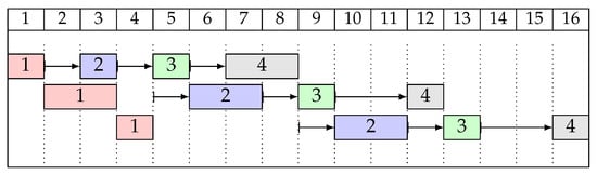
Example 2.
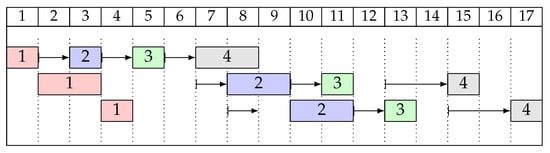
Consider the instance with , and processing times and setup times from Table 2. The order of setups is feasible for that instance. A left-shifted schedule for solution , with , is shown as a Gantt chart in Figure 1. Note that is not an optimal solution. For example, the first setup on machine 2 could be performed earlier (during the third operation on machine 1).
Table 2.
Problem instance from Example 2 for and .
Figure 1.
The left-shifted schedule for the instance from Example 2 and .
4. Problem Properties
In this section, we will formulate several problem properties, particularly the ones regarding the solution space. We start by demonstrating the solution representation using mathematical concepts of lattice paths. We then discuss the number of feasible solutions and the ways to compute it. We formulate two theorems that can be employed in solving methods: an elimination property for skipping certain solutions and a refinement procedure that can improve solutions. Finally, we discuss what portion of the solution space can be skipped by use of the formulated properties.
4.1. Lattice Path Solution Representation
As it was demonstrated in the previous section, some orders of setups are infeasible. To better illustrate the nuances of the solution feasibility in the researched problem, we will introduce the lattice path representation of a solution.
Formally, a lattice path is a sequence of points in , where the difference between any pair of consecutive points , is in a predefined set. Elements of the set are called steps. Here, the set is a standard basis and . One can associate each step , with an act of a setup being performed on machine a. Consider lattice path L from to , consisting of steps in . Each point in this path can be interpreted as a state of a production system with setups already performed on machine a. Then, since there are steps to be performed on each machine, each L represents a unique sequence of setups.
Example 3.
Consider a problem size , and a setup order . The transformation from to the corresponding L can be performed as follows. Start building the path from (the number of dimensions ). Then, for each element in , build sequentially a new point in L by adding 1 to the coordinate given by value of of the previous point. Refer to the equations below:
The reasoning can be reversed to calculate the corresponding to L.
The introduced lattice paths can describe not only feasible setup orders, but also infeasible ones. The problem Constraints (1)–(6) can be directly translated into the domain of lattice paths, by limiting admissible paths to ones consisting of elements in
The interpretation of Equation (13) is that, at any time, the number setups performed on machine a cannot be greater than the number of setups performed on previous machines plus one. Note that does not put direct constraints on a maximum and a minimum number of setups performed on any machine (i.e., constraint ). Such constraints are represented in the set of feasible steps, as well as in the described lattice paths’ start- and endpoints.
4.2. Counting Feasible Solutions
With the lattice path solution representation introduced, one can easily calculate the number of different solutions for a given n and . The following Lemma 1 was first demonstrated by Gnatowski et al. []. Here, however, we will show a proof that will be derived from the general case described in (13).
Lemma 1
(Number of feasible solutions, []). Consider a problem instance with machines and operations. The number of different feasible setup orders is given by the n-th Catalan number
Proof.
The relation between Catalan numbers and the number of feasible setups can be explained in multiple ways. One can use an analogy to the problem of finding the number of possible legal sequences of parentheses; to several different Dyck words-related problems; or to more or less general lattice paths’ analysis (see, for example, a paper by Stanley []). Here, we will explore on the last mentioned possibility, as it also provides some insight into the multi-machine variant of the problem.
For , Equation (13) becomes
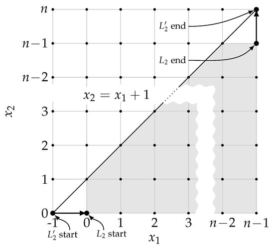
Equation (15) limits the admissible lattice paths from to in , to the ones weakly below line . Such paths will be called paths (as shown in Figure 2).
Figure 2.
Relation between a number of feasible and Catalan numbers. Grey area represents admissible points in paths.
Consider lattice paths from to , with steps in , staying weakly under . In any , the first and the last step are fixed (bold arrows in Figure 2). Therefore, the number of different paths is equal to the number of different paths. Now, by translating the first axis by 1, the starts in and ends in , staying weakly under . The problem of finding the number of different paths defined as such is well known, and has a solution of . For the proof of this fact, as well as other occurrences of Catalan numbers in mathematics, refer to []. □
While for , the number of different feasible solutions can be computed using (14), the case of is much harder. The reasoning from the proof of Lemma 1 cannot be trivially applied for any , even though generalizations for multi-dimensional Catalan numbers exist (see, for example, papers by Haglund [] or Vera-López et al. []).
The constraints on lattice path defined by are relatively complex and—to our knowledge—cannot be addressed by lattice path analysis methods (refer to e.g., a paper by Krattenthaler []) to obtain a useful closed-form expression for computing . On the other hand, recursive formula can be easily obtained and used as a basis for a Dynamic Programming (DP) algorithm, calculating the number of feasible solutions for any .
An outline of the proposed DP method is shown in Algorithm 1. A subproblem given by any is defined as finding a number of different lattice paths from to , satisfying (13). Observe that it is equal to the number of different paths from to each point , where is any point in that can be stepped back from (i.e., ). For example, for , admissible . Different candidates for are created in line 7, while in line 8, it is determined whether they are in . Lastly, a degenerate subproblem has solution of 1, and constitutes a stop criterion for the recurrence (line 3).
Property 1.
Algorithm 1 runs in time, using memory.
Proof.
First, let us count the number of recursive calls of CountSolution. Since the result for each unique is eventually stored in mem, the number of calls and the memory complexity of mem cannot be greater than a cardinality of
where the latter set reflects origin and destination points for the lattice path L. In another words, mem must be able to store solutions to the subproblems corresponding to each point that can appear in L. A simple upper bound for such is obviously , which is the cardinality of the latter set. This allows mem to be a continuous block of memory registers, since it takes to initialize them (line 1). The memory block can then be indexed similarily to C++ arrays, i.e., mem() is understood as mem(), where
Equation (17) is a simple one-to-one mapping of all possible nodes of the considered lattice paths to numbers . The mapping is analogous to a flat array index for multidimensional arrays. The index notation is used to accelerate some computations, taking advantage of an unbounded capacity of a single memory cell (each memory cell of an assumed abstract machine can hold any integer). In a constant time, one can not only access or modify any element of represented by , but also copy , which is not possible for directly.
| Algorithm 1: Counting feasible solutions |
| Data: , a point in . Result: : number of feasible solutions (paths from to in ).  |
Next, let us derive the computational complexity of a single CountSolution call. Lines 3–6 can be conducted in time. Although the computation of the index of takes time, any change in a constant number of elements in can be reflected in in constant time. Therefore, lines 9 and 15 take time. Line 10 can be conducted in time, by using cumulative minimum from line 6. Memory access in lines 11 and 13 can also be conducted in time, using precomputed index —resulting in an overall time complexity of . Memory complexity of a single CountSolution run is .
Overall, the computational complexity of the proposed algorithm is
The memory complexity is
□
A tighter bound can probably be demonstrated for the cardinality of (16) (by a factor of ). Then, however, one could not use a simple index to access memory, leading to a potentially worse computational complexity.
Because of the time and memory complexities, Algorithm 1 performs best when . Such an assumption is usually realistic. Even then, the algorithm can only be used to compute for small and medium instances. Table 3 summarizes the differences between and for several n and m combinations. In particular, for , the can be calculated directly
Clearly, the number of feasible solutions is significantly smaller than the total number of solutions.
Table 3.
Relation between the number of feasible setup orders and the total number of setup orders.
4.3. Elimination Property
In this section, we will discuss the elimination property, which can be used for a quick detection of suboptimal solutions or to potentially improve a solution (as shown in Section 4.4). The property relates to the consecutive setups performed after the same job—constituting a block.
Definition 1.
For solution , let be a k-th node of the lattice path corresponding to , i.e., denotes how many setups were performed on machine a after setup was completed. Let be an h-element subsequence of subseqeuent setups from starting at element k. Subsequence will be called a block of setups in solution (in short, a block) if and only if:
- 1.
- All setups in are performed on a different machine:
- 2.
- All setups in are performed after the same job:
- 3.
- The length h of the block is maximal i.e., of length starting at k is not a block.
- 4.
- Blocks partition the sequence , i.e., each element belongs to exactly one block.
We will illustrate the above definitions with an example.
Example 4.
Consider the following solution:
We start with lattice path node . We then perform . All setups are on different machines and after the same job (, thus is the first block. Note that we cannot define the first block as , because setups are not on different machines. We are now on lattice node . The next block cannot be , because . Thus, , leading to . Similarly and not because . This leads to node . Next, the block cannot be because , but it can be , leading to node . Next, we cannot have a block (machines are not different) or (; thus, the next two blocks will be and leading to nodes and then . Finally, we have , as all elements are different and , leading to . Thus, solution contains seven blocks, as marked by the brackets below.
With the blocks defined, the elimination property can be formulated. The property is a generalization of the result presented by Gnatowski et al. [], for any .
Theorem 1
(Elimination property). Let be a feasible solution, with two consecutive setups , , in a block of job ; such that . Then, a solution , where the order of the setups is reversed,
is feasible and .
Proof.
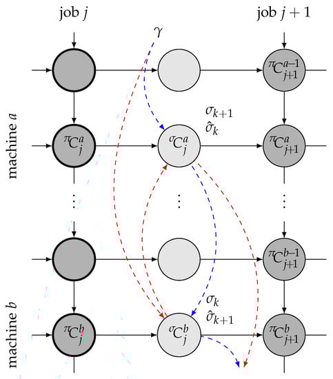
The proof is based on an analysis of left-shifted schedules build from both and . The elements of the schedule build from are denoted with hats (, , etc.). Moreover, let denote the completion time of setup , which is unaffected by the swap. The notation is presented in Figure 3.
Figure 3.
Illustration for the proof of Theorem 1. Solid arrows represent technological and machine constraints. Dashed arrows represent setup order (red for and blue for ). Dark grey circles represent jobs, while light grey circles represent setups.
First, let us identify elements of schedule not affected by the change in the order of setups. Since k-th setup in the original solution is performed on machine b, then by the time the setup can start, the first b operations of job j must be already performed before the setup is started (marked in bold in the figure). Therefore, and remain constant for both setup orders. As a result, the completion time of setups in performed after job j on machines , can only be affected by a change in completion time of -th setup. The change can be expressed as , where
Then,
Since , we have and the completion time of -th setup cannot increase in . As a result, the operations in job preceding operations on machines a and b cannot be delayed, thus and . Therefore, if also operations in job performed on machines a and b can only start earlier, then makespan also can only decrease. We check that further.
Let us discuss the change in completion time of job on machine a,
Knowing, that , we only need to calculate
Since , then the value of (28) is non-negative and therefore and .
Next, let us discuss the change in completion time of job on machine b. Since , we have
Since we know that and , then also .
To sum up, it was proven that in the left-shifted schedule build for , completion time of jobs on machines can only decrease compared to the schedule build for . The same can be said about completion time of -th setup. Therefore, all further jobs and setups can only be performed earlier, resulting in . □
Theorem 1 allows to detect potentially suboptimal solutions. Since the described transformation cannot lead to an increase in makespan, any that fulfills conditions of Theorem 1 (i.e., satisfies the elimination property) can be safely eliminated from the solution space, without the risk of removing all optimal solutions.
4.4. Refinement Procedure
Theorem 1 provides tools for reducing the size of the solution space. However, it can also be observed as a way to potentially improve a solution, by applying a swap move on the setups satisfying the elimination property. A single solution can contain multiple such setup pairs. Moreover, the swap can create a new pair of setups satisfying the elimination property, as shown in Example 5.
Example 5.
Consider a problem size of and . Solution is feasible; however, two setup pairs: and , satisfy elimination property. By applying the swap move to the first pair, we obtain solution —now containing a single, new pair satisfying the property. By applying the swap move, we obtain . Once again, the solution contains a pair , . Finally, the swap move can be applied a third time to obtain . The setup order does not satisfy the condition from Theorem 1 and cannot be eliminated. The procedure can be summarized as follows:
The observation above is a basis of a refinement procedure. Given a solution , the procedure performs setup swaps until Theorem 1 cannot be applied anymore. The resulting solution is said to be refined and
Of course, there exist solutions that do not contain any setup pairs satisfying the elimination property. In such a case, no swaps are performed. In Example 5, the solution is the result of refining the solution .
A few questions arise with regards to the refinement procedure, namely, how to detect which swaps should be performed and in what order. Moreover, we would like to know how fast could this procedure be performed. We will answer those questions in the following theorem, using the fact that the procedure resembles the bubble sort algorithm.
Theorem 2
(Block property). For any feasible solution σ, the refinement procedure can be completed in time.
Proof.
First, observe that rearranging setups within a single block does not change the total number of blocks or contents of other blocks. Therefore, the refinement can be applied for each block separately. Consider a block with a length of l. There is only a single order of setups, for which no pair of setups in the block satisfy the elimination theorem—setups ordered increasingly by the machine on which they are performed. The block can be sorted by applying at most swap-moves, chosen according to the elimination theorem (refer to bubble sort results by Cormen et al. [] (p. 40)). As a result, the worst case time complexity of the procedure would be . However, the sorting can be performed quicker in by using Algorithm 2, which sorts all blocks simultaneously. □
| Algorithm 2: Refinement procedure |
| Data: : solution to be refined. Result: : refined solution.  |
The refinement procedure can be utilized to potentially improve the quality of solutions as a part of larger solving algorithm (e.g., similarly to the individual learning procedure in memetic algorithms proposed by Moscato []). The computational complexity of is equal to the complexity of calculating the objective function; thus, the refinement procedure can be used frequently.
4.5. Counting Eliminated Solutions
In order to estimate how much of the solution space can be eliminated, we first discuss the number of setup orders that cannot be eliminated (preserved solutions). For , the number is given by a known, closed-form expression, first proposed in the lemma by Gnatowski et al. [] (without a proof). Here, we present a proof for the lemma.
Lemma 2
(Number of preserved solutions []). Consider a problem size , . The number of feasible solutions not eliminated by Theorem 1 is given by the -nth Catalan number
Proof.
For the elimination property to be applied, two consecutive setups must be performed after the same job, but on different machines. For , it means that the first setup must be performed on machine 2, and the second on machine 1. For that to be possible, all the setups between previous jobs must already be performed. Such a condition corresponds in the domain of lattice paths to the points on line. Then, step (setup performed on machine 2, against elimination property) moves the lattice path above , and step keeps the lattice path below . Therefore, the elimination property limits the admissible lattice paths from to , to stay weakly below the line. The number of such paths is given by . □
The Lemma 2 allows one to easily obtain the number of preserved solutions for , and thus the number of eliminated solutions.
Theorem 3
(Eliminated solutions for []). Consider a problem size , . Theorem 1 eliminates 50% to 75% of feasible solutions.
- The proof will be omitted, as it was demonstrated in [].
Since even for calculating and , a closed-form expression is not known; to compute the number of preserved solutions, we will resort to the DP approach again. Algorithm 1 must be modified to check both the elimination property condition and the feasibility. For the modified procedure, refer to Algorithm 3.
| Algorithm 3: Counting preserved solutions |
| Data:: potin in . Result:: number of unique preserved solutions.  |
To allow for checking the elimination property, the machine on which the last setup was performed must be added to the definition of a subproblem. For example, for and , the last setup could be performed on any of the three machines (1, 2 or 3). In the Algorithm 3, the machine the last setup was performed on is stored in .
Property 2.
Algorithm 3 runs in time, using memory.
Proof.
The proof is similar to the proof of Property 1. However, now the number of subproblems is m times larger, since each can be potentially matched with any . It results with both computational and memory complexities greater by a factor of m. □
The Algorithm 3 was used to compute the number of unique preserved solutions, denoted by , for and . Then, an elimination ratio
was calculated. The results are demonstrated in Figure 4. For , only a single setup order is preserved, resulting in high elimination ratios that can be calculated from Equation (14). For , increases with the increase of n, eventually overtaking the value for . For instances with a larger number of machines, the elimination ratio continues to increase steadily, reaching almost for .
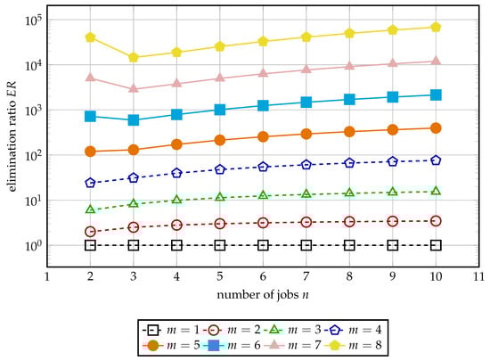
Figure 4.
Elimination ratio for different instance sizes.
5. Solving Algorithms
In this section, three solving algorithms will be described: a MILP-based method, a simple greedy heuristic and a Tabu Search metaheuristic algorithm. The first algorithm will be used later on as a reference to assess the heuristics. Both can also be a part of a two-level algorithm, solving the extended problem for varying the job order.
5.1. Greedy Heuristic
The greedy algorithm was inspired by the NEH algorithm proposed in the paper by Nawaz et al. [] for the FSSP problem. In this case, however, the result of the algorithm is the order of setups for a fixed order of jobs. The method is based on the step-by-step building of a partial solution. First, we set the completion times for the all operations of the first job, as those require no setups. Then, we perform the first setup on the first machine () and the operation after it, while also calculating their completion times. Then, we proceed to insert the remaining elements into , as follows.
Each time, we choose the value of by considering all values that are feasible (given partial setup order up to ). For each such candidate of value a, we compute the completion time of the corresponding setup. In order to do this, we store the completion time of the last setup in throughout the algorithm. For each calculated setup, we then calculate the completion time of the operation after it. Then, as , we choose such value a, for which the computed operation completion time is smallest. The computational complexity of the algorithm depends on the number of setups and machines, and is given by .
Example 6.
Consider the instance from Table 2. For this instance, the greedy solution is constructed as follows. In the first step, we determine the completion time of all three operations of the first job, since they can be processed without any prior setups:
The first setup in the greedy heuristic is always performed after the first operation on the first machine. We perform this setup, which allows us to perform the second operation on the first machine, and we calculate the appropriate completion times:
The next setup can be performed on any machine; thus, we have three candidates, . For each candidate, we evaluate the resulting completion times:
Out of those three possibilities, the minimal value is , so , and . We repeat this procedure for subsequent decisions through . Finally, we obtain solution , shown as a Gantt chart in Figure 5, for which .
Figure 5.
The left-shifted schedule provided by the greedy algorithm for the instance from Table 2.
5.2. MILP Formulation
Mixed-Integer Linear Programming formulation is a popular method for solving optimization problems, especially if a dedicated algorithm does not exist. The MILP formulation used in this paper as a reference algorithm was introduced first in []. Although the aforementioned paper considers a two-machine problem, the formulation can be used for any . It utilizes a relative order to encode setups’ order , resulting in binary variables (relative order of setups performed on the same machine is fixed). We improved the method by utilizing the warm start and providing the solver with upper and lower bounds on the objective function of an optimal solution.
5.2.1. Warm Start
To improve the performance of the algorithm, we used a feasible solution as a starting point. It is especially important for the large instance (with ), where without providing a feasible initial solution, the solver struggled to find any feasible solution at all within a time limit. The starting solution was chosen as a better one from the following two:
- Natural setup order
- Result of a greedy heuristic from Section 5.1.
5.2.2. Objective Function Bounds
The upper bound of the objective function was assigned based on the initial solution from the warm start. The lower bound was calculated from the expression
5.3. Tabu Metaheuristic
Tabu Search (TS), is a well-known local search metaheuristic proposed by Glover [,], which uses a short- and (optionally) a long-term memory to avoid being trapped in a local optimum. Due to its deterministic nature and good performance in practice, it is one of the most commonly used metaheuristic methods, with applications ranging from scheduling (Bożejko et al. []), through knapsack problem (Lai et al. []), model selection (Marcoulides []), or even data replication in cloud environments (Ebadi and Jafari Navimipour []). A general pseudocode of our TS is shown in Algorithm 4. Below, we will describe the most important features of our implementation.
| Algorithm 4: Tabu Search pseudocode |
| Data:: initial solution. Result:: best solution found.  |
5.3.1. Initial Solution and Stopping Condition
The initial solution was the same as for the MILP (best out of “natural” and “greedy” constructive heuristics). The choice of the initial solution is not very impactful, TS can generally provide similar results starting from the worse initial solution, provided the number of iterations is a bit higher. The algorithm stops when the time limit MaxTime is reached.
5.3.2. Neighbourhoods
The neighborhood a of solution is defined as the set of solutions that can be created from by applying a pre-defined move. In our implementation, we considered the insert move . When this move is applied on , it creates neighboring solution by removing from it element and inserting it before element . For example, performing move on the solution from Example 2 would result in:
Normally, the insert neighborhood contains solutions. However, we apply several rejection rules, which may limit the neighborhood size we need to evaluate:
- We ignore moves where , as those moves do not change .
- We ignore moves where , where is an algorithm parameter that defines the width of the neighborhood. We include this parameter, because the full neighborhood search is very costly (i.e., ).
- We reject insert moves that results in infeasible solutions and (optionally) satisfy elimination property and can be eliminated. This operation is faster than evaluating the objective function, and can be potentially conducted in constant time, assuming that the lattice path corresponding to the initial solution is known.
The move leading to the solution with the lowest makespan is chosen (unless it is forbidden, see the next paragraph for details). Optionally, the solution is then refined by the procedure, as described previously in Section 4.4.
5.3.3. Tabu List
We employed a short-term tabu list memory that stores forbidden moves. Solutions created by such moves are ignored unless they are better than the current value of . The tabu list was implemented as a matrix T of size , enabling all tabu list operations in time . The algorithm parameter , called cadence, determines for how many iterations the moves stay forbidden. Based on preliminary research, we chose . Note that when move is performed, the reverse move also becomes forbidden.
5.3.4. Backjumps
Even with the tabu list mechanism in place, the algorithm can still enter a cycle. To alleviate this problem, we used a long-term memory in the form of a list. Every time is updated, we add to the list a triple of: (1) a copy of current solution , (2) a copy of the current tabu list; and (3) the move that led to (not its reverse). If we reach MaxNoImprove iterations without improving , then we perform a backjump. This is conducted by replacing the and tabu list with their copies in the most recent element of the long-term memory list. Algorithm then proceeds normally, except that during the next iteration, we cannot choose the move that was saved in the memory (this prevents TS from following the same branch). After each backjump, we remove the last element of the long-term memory list. If MaxNoImprove is reached and the list is empty, then instead of performing a backjump, we simply restart the search process by setting to a random, feasible solution. Based on preliminary research, we chose .
6. Experimental Results
In this section, we describe the computer experiments on the effectiveness of the proposed solving methods on different instance types.
6.1. Experimental Setup
We conducted tests on the following three algorithms described earlier:
- MILP
- a commercial solver using the MILP formulation of the problem from Section 5.2;
- TabuA
- TS method from Section 5.3, that does not use elimination property to reject neighbors, but uses refinement procedure to improve the best neighbor;
- TabuB
- TS method from Section 5.3, that uses elimination property to reject neighbors.
The TabuA and TabuB algorithms were written in C++ programming language and compiled using g++ version 9.3.0 (with -O3 compilation flag). The MILP formulation was written in Julia programming language version 1.5.3 and employed the Gurobi solver version 9.1.1.rc0 with the default parameters and presolver turned on.
The experiments were run on a machine with 64-core AMD Ryzen Threadripper 3990X processor with 2.9 GHz clock and 64 GB of RAM. Each algorithm used only one CPU core. The experiment was run under a Windows 10 Pro operating system with Windows Subsystem for Linux.
6.1.1. Test Instances
We prepared 120 test instances by the use of a modified version of the FSSP instance generator proposed by Taillard []. We use the same random number generator as Taillard, which is meant to provide integer numbers from uniform distribution . Both operation processing times and setup times were drawn from this distribution. We first generated processing times, identical to Taillard. Then, we generated—without reseeding the random generator—all setup times, starting with the first machine. We generated setup times for each possible job pair; however, only a single pair is used, as the order of jobs is fixed. We generated 10 instances for each of the following size groups (): , , , , , , , , , , , . All instances were given identifiers from 1 to 120. All generated instances are available in the Supplementary Materials to this paper.
6.1.2. Evaluation Method
To measure the quality of the solutions provided by the algorithms, we calculated the percentage relative differences between their quality and the quality of reference solutions—called short gaps. In other words, the gap for a solution is defined as:
where is a reference solution. Generally, we chose to be the best known solution in a given context.
6.2. Width of the Neighborhood
First, we investigated how the width of the neighborhood W affects the performance of the TS algorithm. We ran the TabuA algorithm with for all 120 instances. For each instance, the algorithm was run 100 times, and each time W was set to a different value, equal to a given fraction of the maximum possible neighborhood width. For example, for and , the value of W is in . Then, a 50% width corresponds to W = 145. The reference solution for computing the gap was the best among all 100 runs for each instance. The resulting gaps, averaged over all instances, are shown in Figure 6.
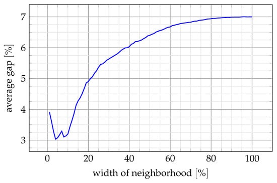
Figure 6.
Impact of the neighborhood width on the gap.
Higher values of W provided considerably worse results, i.e., a larger neighborhood size does not compensate the larger time required to evaluate it. Thus, lower values of W are preferred. However, a very small neighborhood size also leads to a larger gap. Such results are to be expected, as in high quality solutions, most setups are close to their initial positions in the order generated by the starting procedure, and wide inserts are rarely required. On the other hand, a very narrow neighborhood requires multiple TS iterations to perform any significant change in . Based on this observation, we set W to 10% of the maximum neighborhood width in the following experiments.
6.3. Performance of the Algorithms
In this experiment, we have evaluated the performances of the MILP formulation and the TabuA and TabuB metaheuristics, which utilize the problem properties. In order to correctly compare such different solving methods, we opted to use the same stopping condition—a time limit. Since we intend for the solving methods to be applicable as sub-procedures for solving a two-level problem, the short running time is crucial. Thus, we decided to test several short time limits
seconds. Although the times are the most practical in the context of a two-level problem, we considered times up to 100 s to better evaluate how the solving methods converge. For each instance, the reference solution was the best one found by any algorithm in 100 seconds (the makespans of the reference solutions can be found in the Supplementary Materials). The results obtained are shown in Table 4.
Table 4.
Average gap [%] for the MILP, TabuA and TabuB methods for different instance size groups and time limits. Best values for each instance size and time limit are underlined. Rows “Diff” contain performance differences (gains) between running times 100 and 1.
For smaller instances (up to 3 machines, under around 60 operations), the MILP formulation is consistently better or on-par with any TS algorithm, regardless of the time limit. In fact, the solver frequently reported for the returned solutions to be optimal and therefore unbeatable by TS. However, for larger, industry-size instances, the TS algorithm performs better than MILP. Once again, this effect is consistent over all time limits.
Comparing the two TS algorithm variants, TabuB (which makes a wide use of Theorem 1) is consistently better or on-par with TabuA (which uses only the refinement procedure). For larger running times (), both TS algorithms start to provide similar results. This demonstrates that, given enough running time, both versions of the TS algorithm converge to solutions of a similar quality. However, the TabuB variant is superior in convergence speed, outperforming TabuA for and staying on-par with it for . This is easily observed in the last rows of the table, showing the difference (gain) between and time limits. For TabuB, the values are close to 0, meaning the algorithm does not benefit from a higher running time, while still equaling or outperforming TabuA.
Finally, to better visualize the improvements each method makes within the 100 s, we shown in Figure 7 and Figure 8 the relation between the best solution found and time for 6 exemplary instances. The performance of MILP was recorded for seven different time limits (see (47)) set within the solver, while for TS algorithms, a timestamp of each improvement was recorded. The plots confirm that TabuB method converges much faster than TabuA, while the MILP formulation still makes improvements when both TS algorithms have almost converged. Moreover, for some large instances (e.g., instance 78, refer to the figure), even 100 s is not enough for a MILP formulation to improve its starting solution, while TS algorithms converge in under 2 s. On the other hand, in several cases all algorithms failed to make any significant improvements. This, however, mostly happened for smaller instances, where the initial solutions are near-optimal.
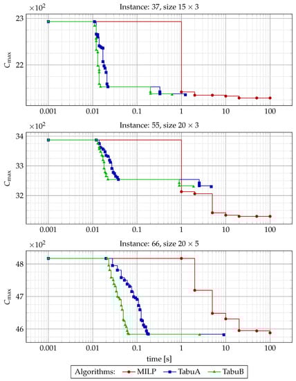
Figure 7.
with regards to running time for the solving methods and 3 exemplary problem instances. For TabuA and TabuB, each mark represents a new best solution found, while for MILP, marks correspond to time limits set for the solver.
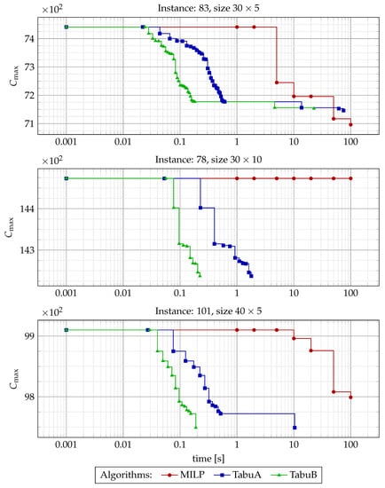
Figure 8.
with regards to running time for the solving methods and 3 exemplary problem instances. For TabuA and TabuB, each mark represents a new best solution found, while for MILP, marks correspond to time limits set for the solver.
7. Conclusions and Future Work
In the paper, we considered a single-server permutation Flow Shop manufacturing process. We divided the full problem into two levels and tackled the second level, i.e., finding an optimal order of disjoint setups for a given, fixed order of jobs.
We presented a mathematical model of the considered problem, including a compact solution representation. Then, we formulated several problem properties. We demonstrated an interesting connection between Catalan numbers and the number of feasible solutions for two machines. We also discussed the challenge of generalizing this result for more machines, despite several generalizations of the Catalan numbers existing. With a lack of a closed-form expression, we proposed a Dynamic Programming algorithm for the task, with a time complexity of . Furthermore, we formulated an elimination property that allows to detect and skip suboptimal solutions. For 10 jobs and 6 machines, the property allows one to disregard almost 99.9% of the solution space. This property was then used to develop an efficient refinement procedure, which can be applied to potentially improve any feasible solution in a time as short as a time required to evaluate it.
To solve the problem, we proposed three algorithms: a Mixed-Integer Linear Programming (MILP) formulation and two variants of the Tabu Search (TS) metaheuristic, implementing the identified properties. The solving methods were then tested empirically on instances based on Taillard’s generation scheme. The MILP formulation was the best for smaller instances (up to 50–60 operations), allowing to obtain optimal or near-optimal solutions. For larger, industry-size instances, the TS algorithms outperformed MILP (which was sometimes unable to improve the starting solution at all). Between the two TS variants, the one utilizing elimination property converged faster than the variant that used only the refinement procedure, usually finding good solutions in under 1 s. A good performance together with short running time proved the usefulness of the proposed method as a part of a larger, two-level heuristic for a full problem.
For future work, we consider three research directions. First, we want to tackle the full, two-level problem, optimizing both the order of setups and the order of jobs. Second, we want to generalize the problem shown in this paper, by allowing for a fixed number of setups to be performed at the same time (multi-server). Third, we want to extend our research concerning the connection between the number of feasible setup orders and lattice paths, in order to obtain a closed-form formula for the size of the solution space.
Supplementary Materials
The following supporting information can be downloaded at: https://www.mdpi.com/article/10.3390/pr10091837/s1.
Author Contributions
Conceptualization, A.G. and J.R.; methodology, A.G., J.R. and R.I.; software, A.G., J.R. and R.I.; validation, A.G. and J.R.; formal analysis, A.G.; investigation, A.G., J.R. and R.I.; resources, A.G.; data curation, A.G., J.R. and R.I.; writing—original draft preparation, A.G., J.R. and R.I.; writing—review and editing, A.G., J.R. and R.I.; visualization, A.G. and R.I. All authors have read and agreed to the published version of the manuscript.
Funding
This research received no external funding.
Data Availability Statement
Not applicable.
Conflicts of Interest
The authors declare no conflict of interest.
Abbreviations
The following abbreviations are used in this manuscript:
| FSSP | Flow Shop Scheduling Problem |
| SIST | Sequence-Independent Setup Times |
| SDST | Sequence-Dependent Setup Times |
| MILP | Mixed-Integer Linear Programming |
| GA | Genetic Algorithm |
| TS | Tabu Search |
| JSSP | Job Shop Scheduling Problem |
| IG | Iterated Greedy |
| DP | Dynamic Programming |
References
- Johnson, S.M. Optimal two- and three-stage production schedules with setup times included. Nav. Res. Logist. Q. 1954, 1, 61–68. [Google Scholar] [CrossRef]
- Neufeld, J.S.; Schulz, S.; Buscher, U. A systematic review of multi-objective hybrid flow shop scheduling. Eur. J. Oper. Res. 2022. [Google Scholar] [CrossRef]
- Komaki, G.M.; Sheikh, S.; Malakooti, B. Flow shop scheduling problems with assembly operations: A review and new trends. Int. J. Prod. Res. 2019, 57, 2926–2955. [Google Scholar] [CrossRef]
- Miyata, H.H.; Nagano, M.S. The blocking flow shop scheduling problem: A comprehensive and conceptual review. Expert Syst. Appl. 2019, 137, 130–156. [Google Scholar] [CrossRef]
- Rossit, D.A.; Tohmé, F.; Frutos, M. The Non-Permutation Flow-Shop scheduling problem: A literature review. Omega 2018, 77, 143–153. [Google Scholar] [CrossRef]
- Ruiz, R.; Maroto, C.; Alcaraz, J. Solving the flowshop scheduling problem with sequence dependent setup times using advanced metaheuristics. Eur. J. Oper. Res. 2005, 165, 34–54. [Google Scholar] [CrossRef]
- Babou, N.; Rebaine, D.; Boudhar, M. Two-machine open shop problem with a single server and set-up time considerations. Theor. Comput. Sci. 2021, 867, 13–29. [Google Scholar] [CrossRef]
- Pongchairerks, P. A Two-Level Metaheuristic Algorithm for the Job-Shop Scheduling Problem. Complexity 2019, 2019, 8683472. [Google Scholar] [CrossRef]
- Bożejko, W.; Gnatowski, A.; Idzikowski, R.; Wodecki, M. Cyclic flow shop scheduling problem with two-machine cells. Arch. Control Sci. 2017, 27, 151–167. [Google Scholar] [CrossRef][Green Version]
- Brucker, P.; Knust, S.; Wang, G. Complexity results for flow-shop problems with a single server. Eur. J. Oper. Res. 2005, 165, 398–407. [Google Scholar] [CrossRef]
- Hamid, M.; Nasiri, M.M.; Werner, F.; Sheikhahmadi, F.; Zhalechian, M. Operating room scheduling by considering the decision-making styles of surgical team members: A comprehensive approach. Comput. Oper. Res. 2019, 108, 166–181. [Google Scholar] [CrossRef]
- Rudy, J.; Smutnicki, C. Online scheduling for a Testing-as-a-Service system. Bull. Pol. Acad. Sci. Tech. Sci. 2020, 68, 869–882. [Google Scholar] [CrossRef]
- Baykasoğlu, A.; Ozsoydan, F.B. Dynamic scheduling of parallel heat treatment furnaces: A case study at a manufacturing system. J. Manuf. Syst. 2018, 46, 152–162. [Google Scholar] [CrossRef]
- Rudy, J.; Rodwald, P. Job Scheduling with Machine Speeds for Password Cracking Using Hashtopolis. In Theory and Applications of Dependable Computer Systems; Zamojski, W., Mazurkiewicz, J., Sugier, J., Walkowiak, T., Kacprzyk, J., Eds.; Springer International Publishing: Cham, Switzerland, 2020; pp. 523–533. [Google Scholar]
- Rudy, J. Cyclic Scheduling Line with Uncertain Data. In Lecture Notes in Computer Science (Including Subseries Lecture Notes in Artificial Intelligence and Lecture Notes in Bioinformatics); Springer: Cham, Switzerland, 2016; pp. 311–320. [Google Scholar] [CrossRef]
- Zeng, Z.; Hong, M.; Man, Y.; Li, J.; Zhang, Y.; Liu, H. Multi-object optimization of flexible flow shop scheduling with batch process—Consideration total electricity consumption and material wastage. J. Clean. Prod. 2018, 183, 925–939. [Google Scholar] [CrossRef]
- Yu, C.; Semeraro, Q.; Matta, A. A genetic algorithm for the hybrid flow shop scheduling with unrelated machines and machine eligibility. Comput. Oper. Res. 2018, 100, 211–229. [Google Scholar] [CrossRef]
- Dios, M.; Fernandez-Viagas, V.; Framinan, J.M. Efficient heuristics for the hybrid flow shop scheduling problem with missing operations. Comput. Ind. Eng. 2018, 115, 88–99. [Google Scholar] [CrossRef]
- Ruiz, R.; Pan, Q.K.; Naderi, B. Iterated Greedy methods for the distributed permutation flowshop scheduling problem. Omega 2019, 83, 213–222. [Google Scholar] [CrossRef]
- Bożejko, W.; Uchroński, M.; Wodecki, M. Blocks for two-machines total weighted tardiness flow shop scheduling problem. Bull. Pol. Acad. Sci. Tech. Sci. 2020, 68, 31–41. [Google Scholar]
- Allahverdi, A.; Gupta, J.N.; Aldowaisan, T. A review of scheduling research involving setup considerations. Omega 1999, 27, 219–239. [Google Scholar] [CrossRef]
- Cheng, T.C.E.; Gupta, J.N.D.; Wang, G. A review of flowshop scheduling research with setup times. Prod. Oper. Manag. 2000, 9, 262–282. [Google Scholar] [CrossRef]
- Reza Hejazi, S.; Saghafian, S. Flowshop-scheduling problems with makespan criterion: A review. Int. J. Prod. Res. 2005, 43, 2895–2929. [Google Scholar] [CrossRef]
- Sharma, P.; Jain, A. A review on job shop scheduling with setup times. Proc. Inst. Mech. Eng. Part B J. Eng. Manuf. 2016, 230, 517–533. [Google Scholar] [CrossRef]
- Zhu, X.; Wilhelm, W.E. Scheduling and lot sizing with sequence-dependent setup: A literature review. IIE Trans. (Inst. Ind. Eng.) 2006, 38, 987–1007. [Google Scholar] [CrossRef]
- Gupta, J.N.; Tunc, E.A. Scheduling a two-stage hybrid flowshop with separable setup and removal times. Eur. J. Oper. Res. 1994, 77, 415–428. [Google Scholar] [CrossRef]
- Rajendran, C.; Ziegler, H. Heuristics for scheduling in a flowshop with setup, processing and removal times separated. Prod. Plan. Control 1997, 8, 568–576. [Google Scholar] [CrossRef]
- Bożejko, W.; Idzikowski, R.; Wodecki, M. Flow Shop Problem with Machine Time Couplings. In Engineering in Dependability of Computer Systems and Networks; Zamojski, W., Mazurkiewicz, J., Sugier, J., Walkowiak, T., Kacprzyk, J., Eds.; Springer International Publishing: Cham, Switzerland, 2020; pp. 80–89. [Google Scholar] [CrossRef]
- Belabid, J.; Aqil, S.; Allali, K. Solving Permutation Flow Shop Scheduling Problem with Sequence-Independent Setup Time. J. Appl. Math. 2020, 2020, 7132469. [Google Scholar] [CrossRef]
- Gupta, J.N.; Darrow, W.P. The two-machine sequence dependent flowshop scheduling problem. Eur. J. Oper. Res. 1986, 24, 439–446. [Google Scholar] [CrossRef]
- Ruiz, R.; Stützle, T. An Iterated Greedy heuristic for the sequence dependent setup times flowshop problem with makespan and weighted tardiness objectives. Eur. J. Oper. Res. 2008, 187, 1143–1159. [Google Scholar] [CrossRef]
- Zandieh, M.; Karimi, N. An adaptive multi-population genetic algorithm to solve the multi-objective group scheduling problem in hybrid flexible flowshop with sequence-dependent setup times. J. Intell. Manuf. 2011, 22, 979–989. [Google Scholar] [CrossRef]
- Fazel Zarandi, M.H.; Mosadegh, H.; Fattahi, M. Two-machine robotic cell scheduling problem with sequence-dependent setup times. Comput. Oper. Res. 2013, 40, 1420–1434. [Google Scholar] [CrossRef]
- Majumder, A.; Laha, D. A new cuckoo search algorithm for 2-machine robotic cell scheduling problem with sequence-dependent setup times. Swarm Evol. Comput. 2016, 28, 131–143. [Google Scholar] [CrossRef]
- Burcin Ozsoydan, F.; Sağir, M. Iterated greedy algorithms enhanced by hyper-heuristic based learning for hybrid flexible flowshop scheduling problem with sequence dependent setup times: A case study at a manufacturing plant. Comput. Oper. Res. 2021, 125, 105044. [Google Scholar] [CrossRef]
- Cheng, T.C.; Wang, G.; Sriskandarajah, C. One-operator-two-machine flowshop scheduling with setup and dismounting times. Comput. Oper. Res. 1999, 26, 715–730. [Google Scholar] [CrossRef]
- Lin, S.W.; Ying, K.C. Makespan optimization in a no-wait flowline manufacturing cell with sequence-dependent family setup times. Comput. Ind. Eng. 2019, 128, 1–7. [Google Scholar] [CrossRef]
- Lim, A.; Rodrigues, B.; Wang, C. Two-machine flow shop problems with a single server. J. Sched. 2006, 9, 515–543. [Google Scholar] [CrossRef]
- Su, L.H.; Lee, Y.Y. The two-machine flowshop no-wait scheduling problem with a single server to minimize the total completion time. Comput. Oper. Res. 2008, 35, 2952–2963. [Google Scholar] [CrossRef]
- Samarghandi, H.; ElMekkawy, T.Y. An efficient hybrid algorithm for the two-machine no-wait flow shop problem with separable setup times and single server. Eur. J. Ind. Eng. 2011, 5, 111–131. [Google Scholar] [CrossRef]
- Cheng, T.C.; Kovalyov, M.Y. Scheduling a single server in a two-machine flow shop. Computing 2003, 70, 167–180. [Google Scholar] [CrossRef]
- Gnatowski, A.; Rudy, J.; Idzikowski, R. On two-machine Flow Shop Scheduling Problem with disjoint setups. In Proceedings of the 2020 IEEE 15th International Conference of System of Systems Engineering (SoSE), Budapest, Hungary, 2–4 June 2020; pp. 277–282. [Google Scholar] [CrossRef]
- Bożejko, W.; Gnatowski, A.; Klempous, R.; Affenzeller, M.; Beham, A. Cyclic scheduling of a robotic cell. In Proceedings of the 2016 7th IEEE International Conference on Cognitive Infocommunications (CogInfoCom), Wroclaw, Poland, 16–18 October 2016; pp. 379–384. [Google Scholar] [CrossRef]
- Iravani, S.M.; Teo, C.P. Asymptotically optimal schedules for single-server flow shop problems with setup costs and times. Oper. Res. Lett. 2005, 33, 421–430. [Google Scholar] [CrossRef]
- Vlk, M.; Novak, A.; Hanzalek, Z. Makespan Minimization with Sequence-dependent Non-overlapping Setups. In Proceedings of the 8th International Conference on Operations Research and Enterprise Systems, SCITEPRESS—Science and Technology Publications, Prague, Czech Republic, 19–21 February 2019; pp. 91–101. [Google Scholar] [CrossRef]
- Okubo, H.; Miyamoto, T.; Yoshida, S.; Mori, K.; Kitamura, S.; Izui, Y. Project scheduling under partially renewable resources and resource consumption during setup operations. Comput. Ind. Eng. 2015, 83, 91–99. [Google Scholar] [CrossRef]
- Tempelmeier, H.; Buschkühl, L. Dynamic multi-machine lotsizing and sequencing with simultaneous scheduling of a common setup resource. Int. J. Prod. Econ. 2008, 113, 401–412. [Google Scholar] [CrossRef]
- Glass, C.A.; Shafransky, Y.M.; Strusevich, V.A. Scheduling for Parallel Dedicated Machines with a Single Server. Nav. Res. Logist. 2000, 47, 304–328. [Google Scholar] [CrossRef]
- Nowicki, E.; Smutnicki, C. A fast taboo search algorithm for the job shop problem. Manag. Sci. 1996, 42, 797–813. [Google Scholar] [CrossRef]
- Stanley, R.P. Catalan Numbers; Cambridge University Press: Cambridge, UK, 2015. [Google Scholar] [CrossRef]
- Haglund, J. The q,t-Catalan Numbers and the Space of Diagonal Harmonics; American Mathematical Society: Providence, RI, USA, 2008. [Google Scholar] [CrossRef]
- Vera-López, A.; García-Sánchez, M.; Basova, O.; Vera-López, F. A generalization of Catalan numbers. Discret. Math. 2014, 332, 23–39. [Google Scholar] [CrossRef]
- Krattenthaler, C. Unimodality, Log-concavity, Real-rootedness And Beyond. In Handbook of Enumerative Combinatorics; Chapman and Hall/CRC: Boca Raton, FL, USA, 2015; pp. 461–508. [Google Scholar] [CrossRef]
- Cormen, T.H.; Leiserson, C.E.; Rivest, R.L.; Clifford, S. Introduction to Algorithms, 3rd ed.; The MIT Press: Cambridge, MA, USA; London, UK, 2009. [Google Scholar]
- Moscato, P. On Evolution, Search, Optimization, Genetic Algorithms and Martial Arts: Towards Memetic Algorithms. In Caltech Concurrent Computation Program, C3P Report. 1989. Available online: https://citeseerx.ist.psu.edu/viewdoc/download?doi=10.1.1.27.9474&rep=rep1&type=pdf (accessed on 6 August 2022).
- Nawaz, M.; Enscore, E.E.; Ham, I. A heuristic algorithm for the m-machine, n-job flow-shop sequencing problem. Omega 1983, 11, 91–95. [Google Scholar] [CrossRef]
- Glover, F. Tabu Search—Part I. ORSA J. Comput. 1989, 1, 190–206. [Google Scholar] [CrossRef]
- Glover, F. Tabu Search—Part II. ORSA J. Comput. 1990, 2, 4–32. [Google Scholar] [CrossRef]
- Lai, X.; Hao, J.K.; Yue, D. Two-stage solution-based tabu search for the multidemand multidimensional knapsack problem. Eur. J. Oper. Res. 2019, 274, 35–48. [Google Scholar] [CrossRef]
- Marcoulides, K.M. Latent growth curve model selection with Tabu search. Int. J. Behav. Dev. 2020, 45, 153–159. [Google Scholar] [CrossRef]
- Ebadi, Y.; Jafari Navimipour, N. An energy-aware method for data replication in the cloud environments using a Tabu search and particle swarm optimization algorithm. Concurr. Comput. Pract. Exp. 2019, 31, e4757. [Google Scholar] [CrossRef]
- Taillard, E. Benchmarks for basic scheduling problems. Eur. J. Oper. Res. 1993, 64, 278–285. [Google Scholar] [CrossRef]
Publisher’s Note: MDPI stays neutral with regard to jurisdictional claims in published maps and institutional affiliations. |
© 2022 by the authors. Licensee MDPI, Basel, Switzerland. This article is an open access article distributed under the terms and conditions of the Creative Commons Attribution (CC BY) license (https://creativecommons.org/licenses/by/4.0/).