Abstract
In a wide range of applications, heating or cooling systems provide not only temperature changes, but also small temperature gradients in a sample or industrial facility. Although a conventional proportional-integral-derivative (PID) controller usually solves the problem, it is not optimal because it does not use information about the main sources of change—the current power of the heater or cooler. The quality of control can be significantly improved by including a model of thermal processes in the control algorithm. Although the temperature distribution in the device can be calculated from a full-fledged 3D model based on partial differential equations, this approach has at least two drawbacks: the presence of many difficult-to-determine parameters and excessive complexity for control tasks. The development of a simplified mathematical model, free from these shortcomings, makes it possible to significantly improve the quality of control. The development of such a model using generative design techniques is considered as an example for a precision adiabatic calorimeter designed to measure the specific heat capacity of solids. The proposed approach, which preserves the physical meaning of the equations, allows for not only significantly improving the consistency between the calculation and experimental data, but also improving the understanding of real processes in the installation.
1. Introduction
Maintaining a predetermined temperature profile in a sample or process object under study is a very common control task. Thermophysical measurements [1,2,3], in which multiple heaters provide heating with zero temperature gradients throughout the sample, would be a good example. A simple proportional-integral-derivative (PID) controller [4] is not optimal since it does not use information about the main source of changes—the current power of the heaters. The control quality can be significantly improved using a thermal process model in the control algorithm. Although the temperature distribution during heating can be described in a detailed three-dimensional model with partial differential equations considering different mechanisms of heat transfer, this approach has at least two drawbacks: the presence of many difficult-to-determine parameters and excessive complexity for control tasks. The development of a simplified mathematical model, free from these shortcomings, allows one not only to achieve a significant improvement in the quality of control but also to identify problem areas in the design. From the point of view of control, the simplest model that provides the necessary accuracy of the description will be optimal.
In trying to build an optimal model by reducing the detail, one faces several obstacles that are difficult to overcome. In addition to the already mentioned problems with determining the parameters of structural elements and heat transfer between them, the real installation almost always differs from the ideas about it embedded in the detailed model. Improving this model requires a large amount of experimental data. The reduction process requires special algorithms to obtain an optimal result, for example, when replacing partial differential equations with ordinary ones. Not relying on a detailed development of the optimal model requires a preliminary numerical assessment of the influence of certain processes on the behavior of the system and the final fine-tuning according to experimental data. As a result, not only the coefficients, but also the equations themselves may change since the influence of individual processes in a real installation may not coincide with our estimates. Creating an optimal model and even automating this process allows the approach known as generative design. The designer formulates the task as a set of conditions or constraints, and the computer offers options for solving the task during an iterative process in which the designer clarifies the formulation of the task, achieving the optimal result. The technology is used to create objects of varied nature but has become most widespread in computer-aided design systems as a means of creating optimal mechanical structures [5]. When creating a mathematical model, the method of generative design consists of the formulation of equations that describe the simulated process by selecting the terms included in them. Methods of such selection for partial differential equations and the evaluation criteria are described in [6,7,8].
The purpose of this work was to demonstrate the application of the generative design method for constructing a model of an adiabatic calorimeter. In the proposed approach, the model is built by “growing” from the original, simple one by successively complicating the equations and refining the coefficients. The fine-tuning of the model is performed while preserving the physical meaning of the heat balance equations. As well as methods for partial differential equations [9,10] and nonlinear dynamics [11,12,13,14], the method is data-driven—it is built based on experimental data and considers only those processes that play a significant role in the behavior of the system.
2. Model Building
Consider constructing such a model using the example of a precision adiabatic calorimeter [3] designed to measure the specific heat capacity of solids in a wide temperature range. The principle of operation of such a device is to measure the temperature increase when a precisely dosed amount of heat is supplied to the cell containing the test sample. The adiabaticity of the process is ensured by a system of active adiabatic shells, the temperature of which is maintained equal to the cell temperature by an automatic control system. A simplified diagram of the calorimeter is shown in Figure 1.
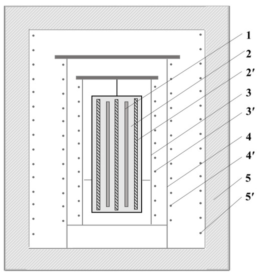
Figure 1.
A simplified diagram of the precision adiabatic calorimeter. Test sample (1) is placed in the silver cell (2) with cell heater (2′); an inner adiabatic shell (3) with a heater (3′) and an outer adiabatic shell (4) with a heater (4′) provide adiabatic conditions; a protective cap (5) with a heater (5′) isolates the system from the environment.
A detailed description of the design of the calorimeter and the equipment used is given in [15]. It also discusses the simplest models used to construct the control system. The measured parameters in the adiabatic calorimeter are the temperatures of the cell, adiabatic shells and protective cap. Appropriate heaters are heat sources. Temperatures are measured by platinum thermometers with individual calibration; the cell is heated by a precision digital power supply. Since the cell and adiabatic shells are made of silver and have high thermal conductivity, in real operation modes, it is possible to neglect the temperature gradients inside them (at least in initial approximations) and consider them isothermal. Considering the nesting of structural elements into each other, heat transfer occurs only between neighboring elements, and in the zero approximation, the system matrix has a simple tridiagonal form:
where Ci is the total heat capacity of the ith structural element; aij–heat transfer coefficients; Pi is the ith heater power; and indices 0–4 refer to the cell, inner and outer adiabatic shells, protective cap, and environment, respectively.
Recall simple facts about the benefits of using the object model in the control process. Suppose, for simplicity, that in the adiabatic calorimeter, the temperatures of the shells should be equal to the cell temperature (due to the presence of heat inflows in a real installation, these temperatures must be slightly different). In the case of a conventional PID controller based on the error value e(t) process variable (in our case, internal shell heater power P1), e(t) is calculated as
The PID controller of the inner shell heater does not know anything about the operation of the other heaters, and when the cell heater is turned on,
there is an inevitable delay in raising the shell temperature (Figure 2).
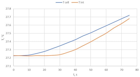
Figure 2.
Cell and internal adiabatic shell temperatures (°C) vs. time (s) at P0‧1(t) cell heater power and common PID controller for internal shell heater.
On the other hand, substituting the condition of equality of temperatures T0 = T1 = T2 into system (1), we find that this condition is met with
Value (4) may not be used directly for the control due to the difference between model (1) and the real device but may be used as an additional feed-forward term on the right side of Equation (2) to reduce the delay and improve the operation of the PID controller. The closer the model is to the real device, the better the control result.
To create an optimal model and determine unknown coefficients, test measurements were carried out with voltage applied to each of the heaters separately, Pi = Pi0‧1(t). In addition, the data obtained during real measurements were used. It should be noted that the calorimeter operates in two modes: fast, reaching the set temperature, and adiabatic heating with smooth supply and removal of power and equality of cell and shell temperatures (Figure 3).
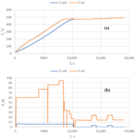
Figure 3.
Cell and internal shell temperatures (a) and heater power (b) during real measurement. Both modes of operation were used—heating to about 500 °C (t < 10,000 s), and adiabatic mode for specific heat measurement (t > 10,000 s).
3. Generating Optimized Model
3.1. Starting Point
To grow an optimized model, the system (1) is used as a “seed”. To simplify the explanation and reduce the size of the article, consider only the first equation of this system.
Coefficients C0 and a01 are calculated from known temperatures T0, T1, and power P0 by using the “least squares” method for the best match between the left and right sides of Equation (5). In other words, minimizing the square of the residual,
where both the derivative and the integral are calculated numerically. A reduced set of only three measurements (Figure 4) is used here as an example.
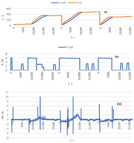
Figure 4.
The data set composed of three real measurements. Cell and internal shell temperatures (a), cell heater power (b), and the residual δP (c).
In addition to the values of the coefficients, their standard deviations (SD) were also calculated and used as an error estimation (Table 1).

Table 1.
Calculated coefficients of Equation (5) and their standard deviations.
To assess how well the model reflects the real processes, standard deviations of the heater power, SD(P0) = 2.72 W, and the residual, SD(δP) = 0.57 W, were calculated. These give the relative error for the starting point, δ = 21%.
3.2. Generative Design. Generalization of Dependencies and Structure
A simple model (1) assumes the constancy of the coefficients. To build a more realistic model, we need to consider the dependence of heat capacity on temperature and the presence of various heat exchange mechanisms. Moreover, the assumption of the interaction of only neighboring structural elements may not correspond to the actual installation.
Sets of heat capacities and heat flow can contain physically meaningful functions or just simply polynomial approximations. In our case, we obtain
where linear regression gives the following coefficients (Table 2).
Table 2.
The coefficients for Equation (4) generalized to (6).
This reduces the standard deviation of the residual by about two-thirds, to SD(δP) = 0.18 W, and the relative error to δ = 6.6%, less than one third of the starting point.
In addition, at this stage, there are no new components corresponding to heat exchange with structural elements other than the inner shell. Thus, if it is present, its role is insignificant.
3.3. Generative Design. Expansion
The equations of the model are essentially the equations of thermal balance, the law of conservation of energy. Thus, a residual other than 0 means a thermal imbalance. The set of random bursts in Figure 4 can be made more convenient for analysis by going from power to enthalpy and using the integral residual:
Just like the peaks in Figure 4c and Figure 5 show, the discrepancy is because the simple model (1) does not describe the fast transient processes in the system since it reduces the entire structure to several large elements. The relationship between the spatial and temporal resolution of the model can be demonstrated by the example of constructing a conservative numerical scheme for the equation of thermal conductivity:
where c, ρ, T, and p are the specific heat, density, temperature, and volumetric heating power, respectively, all dependent on the coordinates and time, and g is the heat flow. At any given time, (7) can be linearized by a Jacobian matrix Jnm.
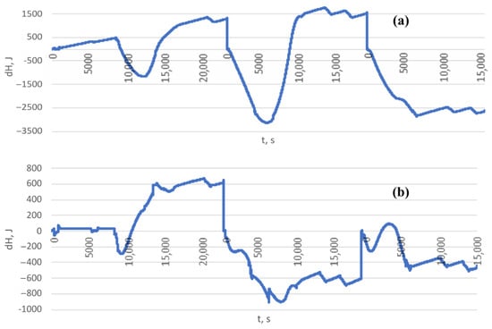
Figure 5.
Residual enthalpy for starting point model (a) and after generalization (b).
The solution of (8) can be described using eigenvalues and eigenvectors of Jnm.
According to (9), the solution contains components with a time constant of . Due to physical reasons, all eigenvalues are not positive, and when. . In other words, the greater the spatial detail, the better the model describes transients.
To build an optimal model, we will consistently add new thermal elements to it in those places where the residual is maximum or close to it. To determine the coefficients, we will use the results of experiments with heating in the form of a Heaviside function:
and we will limit the area of linear regression calculation to the duration of the transient process. We will use the same Equation (5) as a starting point to simplify the presentation. In this case, new calculation gives coefficients (Table 3) that are slightly different from those calculated earlier (Table 1) due to the different regression base.
Table 3.
The coefficients for Equation (5) for heating in the form of a Heaviside function.
The maximum residue—the peak in Figure 6a (step in Figure 6b)—corresponds to the fastest process in the system, turning on the cell heater. Adding an intermediate thermal element within the cell, which can be identified as the actual heater with its own temperature and heat capacity, gives the system (15). With the coefficients of Table 4, this can reduce the residual power by 5 times (Figure 7) and significantly improve the enthalpy residue (Figure 8).
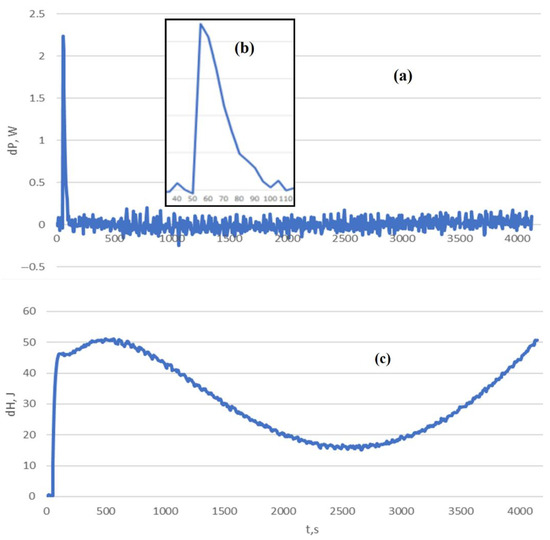
Figure 6.
Residual power (a) with detailed view (b) and enthalpy (c) for Equation (4) with coefficients from Table 3.
Table 4.
The coefficients for Equation (15).
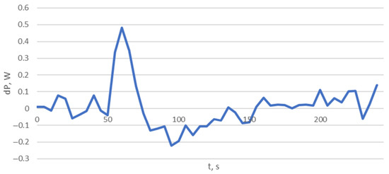
Figure 7.
Residual power for T0 Equation in (15) with coefficients from Table 4.
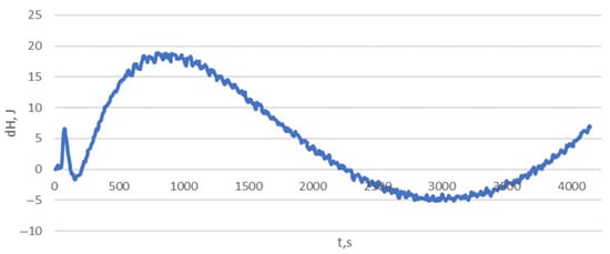
Figure 8.
Residual enthalpy for T0 Equation in (15) with coefficients from Table 4.
To determine what other terms and equations should be added to the system (15), we will perform an approximation of the residual enthalpy with powers of temperatures T0 and T1. The coefficients and their standard deviations are shown in Table 5.
Table 5.
The coefficients for Equation (15) with powers of temperatures T0 and T1.
Residual enthalpy decreases by more than 10 times, as shown in Figure 9.
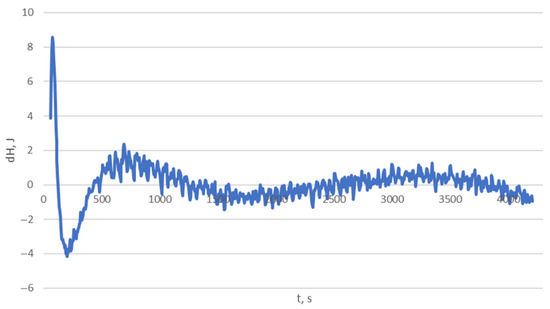
Figure 9.
Residual enthalpy after approximation from Table 5.
Obviously, the approximation of Table 5 contains an excessive number of approximating terms. This is evidenced by a significant relative (about 10%) error of the coefficients. The magnitude of this error can serve as a criterion for choosing the final approximation. After excluding several terms, the relative error of the remaining coefficients is less than 1% (Table 6). Reducing the number of terms practically did not worsen the approximation—the graph of residual enthalpy has no visible differences from Figure 9.
Table 6.
The coefficients for Equation (15) with excluded powers of temperatures T0 and T1.
Since residual enthalpy is an integral characteristic, the equation for T0 must contain derivatives . These terms look like heat capacity correction and appear on the right side of equation for T0 in the system (16) as an additional heat transfer channel.
The dependence on T1 can be understood if we add the last two Equations in (16):
where C0+1 and C1 are both linear functions of the temperature. Due to the large number of coefficients, we did not list them in the table.
This process continues to sequentially remove the main part from the residue step-by-step until the required accuracy is achieved.
The constructed model is conveniently represented as an undirected graph showing the thermal relationship between the installation elements. For example, for system (16), we have Figure 10.
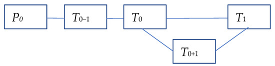
Figure 10.
Topology of thermal relations of the inner part of the calorimeter.
Figure 10 shows that in addition to the thermal conductivity along the air gap, there is a thermal contact between the cell and the inner shell along the suspension and the supply wires. The heater temperature during rapid heating will differ from the cell’s temperature.
The use of the model in the control loop made it possible to maintain the temperature difference between the cell and the inner shell on the measuring heaters with an error of less than 0.01 °C.
3.4. Computing Features
At the starting point and during generalization (systems (1) and (7)), the search for coefficients by the method of least squares was reduced to linear regression since all of the functions on the right side were known. During expansion, unknown temperatures T0−1 in system (15) and T0+1 in (16) appear. In the process of finding the minimum of the total of the square of the residuals, differential equations for these temperatures are solved at each step. Finding the extremum depends on the number of variable parameters; in complex cases, an evolutionary algorithm is used [16]. Adding new variables and equations uses a data segment corresponding to the duration of the transition process.
4. Conclusions
The proposed approach allows building a conservative thermal process model with a clear physical meaning of the equations. A key feature of the approach is the construction of the system by sequential complication and use of the residual enthalpy as a criterion for the correspondence of the model to the experimental data. The constructed model not only improves the quality of control but also clarifies the ideas about the real processes in the installation.
Further work will use deep neural networks to build a model and automate the process of studying the installation with the active formation of optimal test procedures.
Author Contributions
Conceptualization, methodology, software, validation, T.A.A., N.Y.B. and A.Y.L.; formal analysis, investigation, resources, data curation, T.A.K., V.I.K. and V.V.V.; writing—original draft preparation, T.A.A.; writing—review and editing, A.Y.L. and T.A.K.; supervision, project administration, funding acquisition, N.Y.B. All authors have read and agreed to the published version of the manuscript.
Funding
This research was funded by Russian Science Foundation, Agreement 21-11-00296.
Institutional Review Board Statement
Not applicable.
Informed Consent Statement
Not applicable.
Data Availability Statement
The data presented in this study are available on request from the corresponding author. The data is not publicly available due to its purely demonstrative nature.
Conflicts of Interest
The authors declare no conflict of interest. The funders had no role in the design of the study; in the collection, analyses, or interpretation of data; in the writing of the manuscript; or in the decision to publish the results.
References
- Nishiyama, E.; Tsukushi, I.; Fujimura, J.; Yokota, M. Construction of a top-loading adiabatic calorimeter equipped with a refrigerator. Thermochim. Acta 2020, 692, 178151. [Google Scholar] [CrossRef]
- Tan, Z.C.; Shi, Q.; Liu, X. Construction of High-Precision Adiabatic Calorimeter and Thermodynamic Study on Functional Materials. In Calorimetry—Design, Theory and Applications in Porous Solids; Piraján, J.C.M., Ed.; IntechOpen: London, UK, 2008. [Google Scholar]
- Kompan, T.A.; Kulagin, V.I.; Vlasova, V.V.; Kondratiev, S.V.; Lukin, A.Y.; Pukhov, N.F. State Primary Standard of Unit of Specific Heat Capacity of Solids (Get 60-2019). Meas. Tech. 2020, 63, 407–413. [Google Scholar] [CrossRef]
- Li, Y.; Ang, K.H.; Chong, G.C.Y. PID control system analysis and design. IEEE Control Syst. Mag. 2006, 26, 32–41. [Google Scholar]
- Barbieri, L.; Muzzupappa, M. Performance-Driven Engineering Design Approaches Based on Generative Design and Topology Optimization Tools: A Comparative Study. Appl. Sci. 2022, 12, 2106. [Google Scholar] [CrossRef]
- Bykov, N.Y.; Hvatov, A.A.; Kalyuzhnaya, A.; Boukhanovsky, A.V. A method for reconstructing models of heat and mass transfer from the spatio-temporal distribution of parameters. Pisma V Zhurnal Tekhnicheskoi Fiz. 2021, 47, 9–12. [Google Scholar]
- Maslyaev, M.; Hvatov, A.; Kalyuzhnaya, A.V. Partial differential equations discovery with EPDE framework: Application for real and synthetic data. J. Comp. Sci. 2021, 53, 101345. [Google Scholar] [CrossRef]
- Schaeffer, H.; Caflisch, R.; Hauck, C.D.; Osher, S. Learning partial differential equations via data discovery and sparse optimization. Proc. R. Soc. A Math. Phys. Eng. Sci. 2017, 473, 20160446. [Google Scholar] [CrossRef] [PubMed]
- Berg, J.; Nyström, K. Data-driven discovery of PDEs in complex datasets. J. Comput. Phys. 2019, 384, 239–252. [Google Scholar] [CrossRef]
- Rudy, S.H.; Alla, A.; Brunton, S.L.; Kutz, J.N. Data-driven identification of parametric partial differential equations. SIAM J. Appl. Dyn. Syst. 2019, 18, 643–660. [Google Scholar] [CrossRef]
- Qin, T.; Wu, K.; Xiu, D. Data driven governing equations approximation using deep neural networks. J. Comput. Phys. 2019, 395, 620–635. [Google Scholar] [CrossRef]
- Mangan, N.M.; Kutz, J.N.; Brunton, S.L.; Proctor, J.L. Model selection for dynamical systems via sparse regression and information criteria. Proc. R. Soc. A 2017, 473, 20170009. [Google Scholar] [CrossRef] [PubMed]
- Brunton, S.L.; Proctor, J.L.; Kutz, J.N.; Bialek, W. Discovering governing equations from data by sparse identification of nonlinear dynamical systems. Proc. Natl. Acad. Sci. USA 2016, 113, 3932–3937. [Google Scholar] [CrossRef]
- Bongard, J.; Lipson, H. Automated reverse engineering of nonlinear dynamical systems. Proc. Natl. Acad. Sci. USA 2007, 104, 9943–9948. [Google Scholar] [CrossRef]
- Andreeva, T.A.; Bykov, N.Y.; Vlasova, V.V.; Kompan, T.A.; Kulagin, V.I.; Lukin, A.Y. Reference Adiabatic Calorimeter: Hardware Implementation and Control Algorithms. Meas. Tech. 2022, 64, 903–911. [Google Scholar] [CrossRef]
- Maslyaev, M.; Hvatov, A. Multi-Objective Discovery of PDE Systems Using Evolutionary Approach. In Proceedings of the 2021 IEEE Congress on Evolutionary Computation (CEC), Kraków, Poland, 28 June–1 July 2021; pp. 596–603. [Google Scholar]


Disclaimer/Publisher’s Note: The statements, opinions and data contained in all publications are solely those of the individual author(s) and contributor(s) and not of MDPI and/or the editor(s). MDPI and/or the editor(s) disclaim responsibility for any injury to people or property resulting from any ideas, methods, instructions or products referred to in the content. |
© 2023 by the authors. Licensee MDPI, Basel, Switzerland. This article is an open access article distributed under the terms and conditions of the Creative Commons Attribution (CC BY) license (https://creativecommons.org/licenses/by/4.0/).