Influence of Particle Shape on Tortuosity of Non-Spherical Particle Packed Beds

Abstract

Tortuosity in packed beds or porous media is of significant interest in many fields, from geoscience to the chemical industry. Tortuosity plays a significant role in the mass transport in porous media, but also in their residual thermal or electric conductivity when the particles are not conducting. Several predictive models have been proposed to evaluate tortuosity, but there is still a gap when it comes to considering various particle shapes. The preponderance of tortuosity models substantiated in the literature are porosity-dependent while only a few include shape parameters. In this work, we propose a new model with sphericity and porosity to predict the tortuosity based on thermal simulations carried out with non-conducting particles for domains with no wall effect. The beds generated from rigid body simulations are compared and studied for different particle shapes with a sphericity range of 0.65–1. Sphericity showed a significant effect on the tortuosity compared with other 3D shape parameters (numbers of faces, edges, and vertices); therefore, only sphericity has been considered in the new model. The proposed new model is well suited for the porosity range of 0.3 to 0.4. In said ranges, it is an upgrade of the classical Zehner–Bauer–Schlünder (ZBS) model for the effective thermal conductivity of packed beds, with superior performance.

1. Introduction

Diffusion in packed beds or porous media is particularly of interest for chemical reactor design [1,2] and in industrial sectors such as food [3], pharmaceutical [4], and storage technologies [5]. In addition, it is also of importance in the fields of geosciences [6,7], membrane technology [8], water treatment [9], and electrochemical devices [10] like fuel cells [11,12,13] and lithium-ion batteries [14,15]. Gas diffusion or thermal conduction in porous materials is lower than in an unconfined space due to reduced accessible area on the cross-section and increased mass transport path length. Hence, the effective diffusion coefficient, $D_{eff}$, in porous media can be expressed as

$$\frac{D_{eff}}{D_0}=\frac{\epsilon }{\tau },$$

(1)

where $\epsilon$ is the porosity and $D_0$ is the free-space, molecular diffusivity. Tortuosity, $\tau$, is the ratio of the increased tortuous path length to the thickness of the porous medium. Therefore, studying tortuosity in porous media is necessary to deeply understand diffusion. Many studies have regarded tortuosity as a function of the porosity, pore morphology, and specific surface area, $A_{ss}$, of porous media, but not as a function of particle shape parameters, which also have a substantial effect. Hence, it is necessary to investigate the impact of particle shape parameters on tortuosity.

In the literature, tortuosity is defined either as physical tortuosity with respect to different transport phenomena (hydraulic, electrical, diffusional, thermal tortuosity) [16,17] or as geometric tortuosity based on material structure and geometry. Several methods have been reported to capture the geometrical effects: computed tomography with image analysis [18], path tracking methods [19], and various algorithms to find the shortest path [20,21,22]. The physical types of tortuosity are based on numerical simulations: hydraulic tortuosity is considered for fluid flow and was first accounted for in the widely known Kozeny–Carman equation to predict the permeability of porous media [23,24,25], which includes $\epsilon$, $A_{ss}$, $\tau$, and a shape factor (depending on particle shape). In recent times, tortuosity has been mainly computed from streamlined data of fluid flow simulations utilizing the finite volume method [26,27] and the lattice Boltzmann method [28,29], additionally, also by volume averaging approaches [30,31]. On the other hand, electrical, diffusional, and thermal tortuosities use simple transport laws such as Ohm’s law, Fick’s law, and Fourier’s law, respectively, and incorporated in finite volume methods (FVM), finite element methods (FEM), and finite difference methods [7,10,13,32,33]. Fu et al. [17] and Ghanbarian et al. [16], in their detailed reviews of these parameters, concluded that electrical, diffusional, and thermal tortuosity are identical and greater than the geometrical tortuosity. Fu et al. [17] also suggested an empirical model to find diffusional tortuosity from geometrical tortuosity, pointing out that geometrical tortuosity may be more fundamental in nature, supported by [16]. However, in some cases, diffusion has to be described purely based on the diffusional tortuosity, since the deviations can otherwise be significant at lower porosities [17].

Several empirical models have been proposed which rely entirely on porosity [34,35,36,37,38,39,40,41] to estimate tortuosity. In these correlation models, researchers have sometimes introduced special empirical constants based on the grain shape [39,42] or porous structure [43], also named resistivity factors [44,45]. Respective constants are considered adjustable parameters in many applications, but they can lead to significant errors when evaluating tortuosity [17]. Apart from such constants, there is to our knowledge only one theoretical model by Lanfrey et al. [46] which introduced a particle shape parameter, i.e., sphericity, $\varphi$. However, this model was derived for packed beds of identical particles; therefore, it predicted exaggeratedly high values of tortuosity compared with experimental results and other models [16,17].

Despite these numerous models and applications, there is still a significant deficit in our ability to predict the effect of particle shape on tortuosity. The impact of shape must be studied to obtain an accurate model, especially in the field of granular materials and industrial-packed bed systems.

In this work, we concentrate on parameters that can be used to capture the influence of particle shape on tortuosity and, parallelly, to modify the gas diffusion term in the well-known standard empirical model by Zehner, Bauer, and Schlünder (ZBS) for the thermal conductivity of packed beds made of spherical particles [37,47]. In Section 2, we discuss this and some other models of tortuosity that are subsequently used for comparison with numerical results. In Section 3, regarding methods, particle shape and shape parameters are discussed in detail, alongside methods for bed generation, domain selection, and numerical simulation. In Section 4, bed porosity and simulation results on residual bed conductivity and tortuosity are compared with existing models and shape parameters. Finally, sphericity is introduced in the tortuosity equation to obtain a new empirical equation, followed by conclusions.

2. Tortuosity Models

This section discusses some well-established tortuosity models for packed beds. The oldest formulation was proposed by Maxwell for the electric conductance of nonconducting spheres surrounded by a conducting fluid [34]. He provided a porosity–tortuosity relation given by

$$\tau =1+0.5(1-\epsilon ).$$

(2)

Maxwell’s analytical derivation, however, has been carried out for dilute particle systems, i.e., for higher porosity. Better applicable to the low porosity limit might thus be an equation proposed by Weissberg [36] for both mono-disperse and poly-disperse packings of spheres,

$$\tau =1-0.5\ln \epsilon .$$

(3)

Based on numerous experimental results for packed beds and granular systems, Zehner et al. [47] (in German) came up with the equation

$$\tau =\epsilon /\left(1-\sqrt{1-\epsilon }\right)$$

(4)

Underlying data are for different materials, including some poly-dispersed and non-spherical particles, though not precisely characterized. More details on this can be found in a review [37], alongside the equations of the complete thermal conductivity model, which is well known as the ZBS model. Comiti and Renaud [39] proposed a logarithmic model similar to [36] with an additional adjustable parameter, $C$, which may be a function of shape, given by

$$\tau =1-C\ln \epsilon .$$

(5)

A new unit cell approach was proposed by du Plessis et al. [41] for regular, staggered arrays of obstacles in stagnant fluid systems,

$$\tau =(1-\epsilon )(1-\sqrt{1-\epsilon })+\epsilon (1-{(1-\epsilon )}^{2/3}).$$

(6)

The equation had good agreement with experimental results from [43], which were also used in the development of Equation (4) [47]. The only model that explicitly considers a particle shape parameter is from Lanfrey et al. [46], who introduced sphericity into the relation. They treated the tortuous path as a sinusoidal line across the particle’s boundary. The equation obtained was

$$\tau =1.23\frac{{(1-\epsilon )}^{4/3}}{{\varphi }^2\epsilon }.$$

(7)

The mentioned models are later compared with simulation results.

3. Methods

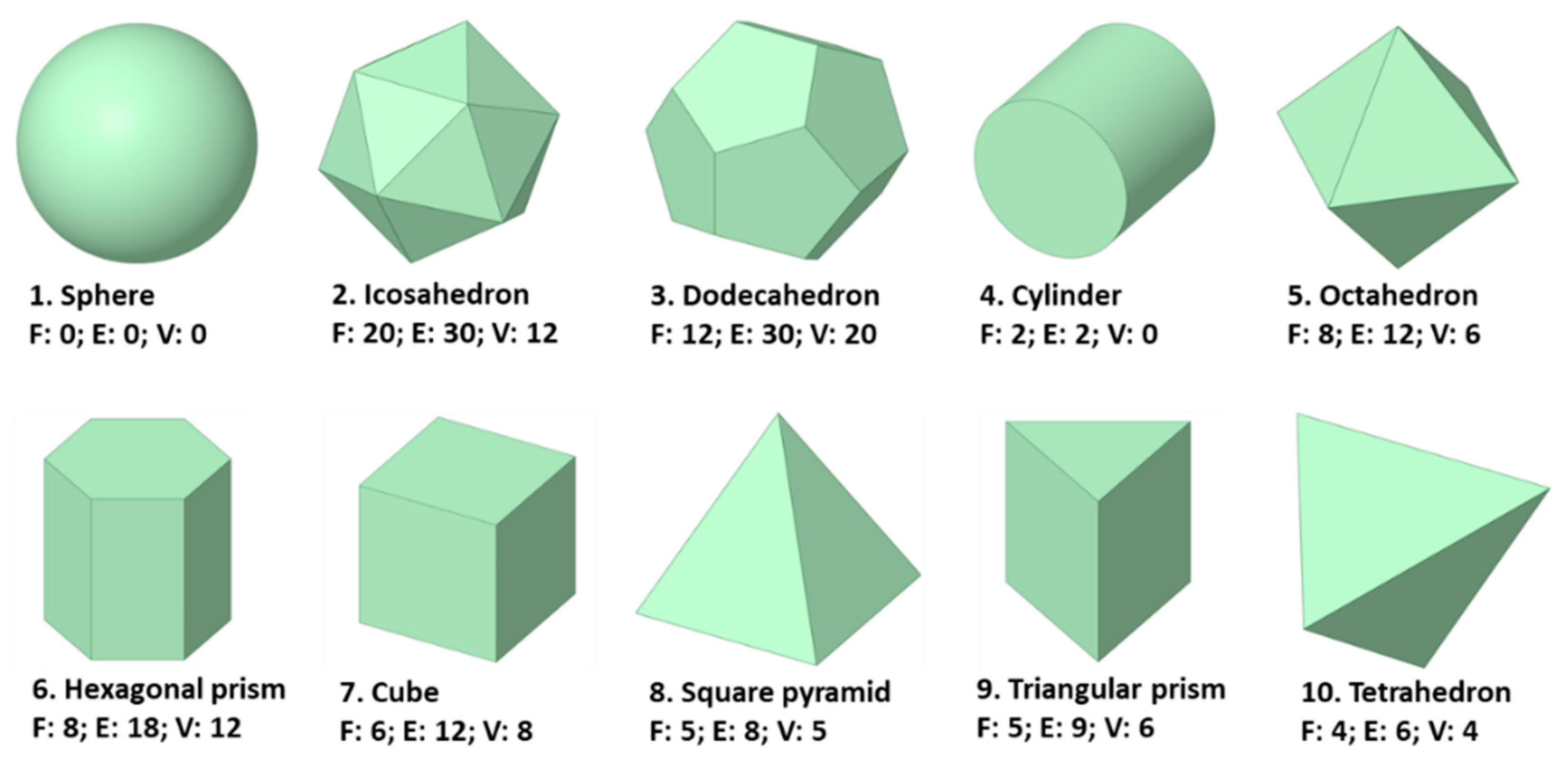
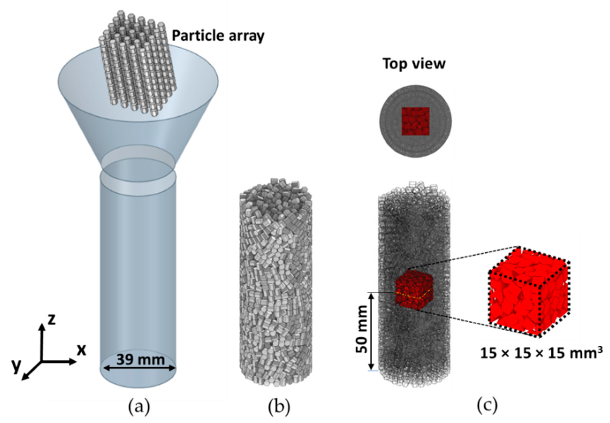
3.1. Particle Shape and Packing Generation

To understand the effect of particle shape on thermal diffusion and to obtain tortuosity relations, ten different shapes were chosen based on their different sphericities, with the volume of the particles kept constant at $V_p$ = 27 mm³ (Figure 1). Sphericity is calculated from the ratio of the equal-volume sphere surface area to the particle surface area,

$$\varphi =\frac{{\pi }^{1/3}{(6V_p)}^{2/3}}{A_p}.$$

(8)

For the different particle shapes presented in Figure 1, the sphericity ranges from 0.671–1 (

Table 1. Overview of sphericity and surface area of all particles together with assigned particle ID ($A_p$ in mm²).

Particle ID	Particle Type	$\mathbf{Surface}\mathbf{Area},{\mathit{A}}_{\mathit{p}}$	$\mathbf{Sphericity},\mathit{\varphi }$
1	Sphere	43.54	1.000
2	Icosahedron	46.34	0.939
3	Dodecahedron	47.81	0.911
4	Cylinder	49.83	0.874
5	Octahedron	51.47	0.846
6	Hexagonal prism	51.59	0.844
7	Cube	54.00	0.806
8	Square pyramid	60.58	0.719
9	Triangular prism	60.79	0.716
10	Tetrahedron	64.85	0.671

). The aspect ratios were selected close to unity; thus, lower aspect ratios of the particles are not considered in this study. All shapes shown in Figure 1 are provided with their 3-dimensional properties. This refers to the number of faces (F), edges (E), and vertices (V). Properties for all shapes are straightforward, except for the sphere and cylinder. The sphere could be considered to have an infinite number of faces with zero surface area each. However, in this work, we will retain the conventional approach that a face must be of finite surface area and flat. Hence, the number of faces for the sphere is taken as zero, and the same for edges and vertices. Similarly, the cylinder is considered to only have two faces and zero vertices. The surface area is provided together with the sphericity in Table 1.

Particle shapes considered in this work, except spherical and cylindrical particles, can be easily represented with a limited number of surfaces, whereas a sphere needs infinite surfaces to be perfectly discretized. Hence, a finite number of 930 small surfaces was used to describe the spherical particle. It has a particle volume that is 0.1% less than the perfect sphere. This is not a significant difference. Likewise, the cylindrical particle volume difference was 0.2% for the application of 924 surfaces.

The packed beds were generated by rigid body simulations using Blender, an open-source and free software for 3D computer graphics [48]. For this purpose, the setup with a funnel of a height of 50 mm, with a bottom opening identical to the cylinder diameter of $D$ = 39 mm and a side angle of 45° (Figure 2a) was used. The particles were dropped into the funnel under gravity along the axial direction. They were placed in arrays of 5 × 5 × 10 tilted by 45° with respect to the vertical axis of the cylinder [49], a total of 12 similar particle arrays were used to fill the cylinder. The rigid body toolbox in Blender was applied to solve the laws of motion and particle–particle interactions [50]. In these Blender simulations, the contact forces were calculated using actual particle surfaces, namely, a triangular surface mesh called STL files; whereas the discrete element method (DEM) was based on the sphere [51]. Many researchers have opted for Blender due to its ability to solve for particles of any polyhedral shape with affordable computational cost [49, 52, 53, 54, 55].

Similar simulation parameters were considered as in [49] with the collision shape being that of the respective convex hull for all forms and spherical for the spherical particles. The collision margin was considered zero, meaning that face-to-face contacts had no gap between the particles. Simulations were run until all particles were settled (Figure 2b). For further thermal simulation, all particle shape packings were generated three times, and residual conductivities were calculated for the small simulation domains as depicted in Figure 2c. These values are later on averaged (see Section 3.2). Similarly, the average bed and domain porosities of the three realizations were used for the following calculations and comparisons.

3.2. Domain and Thermal Simulations

Figure 2 depicts the cubical domain of 15 × 15 × 15 mm³ from the inner region of the bed that was used for the thermal simulations. This domain was selected based on our previous work [49], where cubical particle-packed beds were simulated, and a domain study was carried out using additional micro-computed X-ray tomography (µ-CT) measurement results. The effect of the wall diminishes for $(R-r)/d_p$ > 3.22 at $D/d_p$ = 10.48 ($d_p$ is the diameter of a sphere of equal volume as the particle with $V_p$ = 27 mm³), which is considered in this work. Regarding domain independence, 15 × 15 × 15 mm³ provided the same results as a larger domain [49].

Thermal numerical simulations were performed using a finite element scheme in the commercial software ANSYS—Version 2021 R2. The energy equation was solved until the thermal steady state was achieved. Following model M3 from [56], both phases are in principle conducting. However, a thermal conductivity of ${\lambda }_p$ = 10⁻⁴ W/(mK) for the particles and of ${\lambda }_g$ = 1 W/(mK) for the gas phase were used in the simulations; thus, the ratio $k_p={\lambda }_p/{\lambda }_g$ could be considered so small, as to completely neglect the conduction in the solid phase. The ICEM CFD toolbox from ANSYS was utilized for mesh generation. The mesh was generated based on the cell size of the interface between the phases. Finally, a maximum cell size of 0.1 mm (2.6% of $d_p$) was taken after grid independence studies for all shapes. These are discussed in Section 4.2.1. Temperature boundary values of 50 °C and 20 °C ($\Delta T$ = 30 K) were specified at two opposite faces of the computational domain, with all other faces at adiabatic conditions. Simulations were carried out for different shapes with three different realizations and in the two lateral directions, x and y (refer to Figure 2a). Lateral values were chosen because of the isotropic nature of the beds in respective directions, whereas minor differences may occur in the z-direction (axial direction), as observed in the previous work [49].

The effective thermal conductivity of the beds, ${\lambda }_{bed}$, was calculated using Fourier’s law given by ${\lambda }_{bed}=q_x\Delta x/\Delta T$ or ${\lambda }_{bed}=q_y\Delta y/\Delta T$, where $\Delta x=\Delta y$ is the cubical domain side. For the determination of the heat flux along the direction of heat flow, the volume integral method is often used in FVM simulations, which is different from the nodal average used in our previous work [49]. In the literature, the heat flux is generally calculated from cross-sectional planes either at the boundaries or within the domain, or in FVM by the volume integral method [57,58,59,60]. We compared both methods and found the volume integral method to be more accurate. Hence, the volume integral method has been chosen for this work. The elemental values were extracted from the FEM simulations. Heat flux was calculated by using the equation

$$q_x={\displaystyle \sum _{i=1}^N{q}_{x,i}}{v}_i.$$

(9)

which is the summation of the product of elemental volume fraction $v_i$ and elemental directional heat flux $q_{x,i}$, with $N$ representing the total number of mesh elements.

Note that when the thermal conductivity of the particles can be neglected, the reduced effective thermal conductivity of the bed, $k_{bed}={{\lambda }_{bed}/\lambda }_g$, is equal to the reduced diffusivity of Equation (1). This means it is equivalent to the ratio of porosity and tortuosity $k_{bed}(k_p\to 0)=\epsilon /\tau$. Consequently, direct access to the tortuosity of packed beds of non-spherical particles is provided by the present approach.

4. Results and Discussion

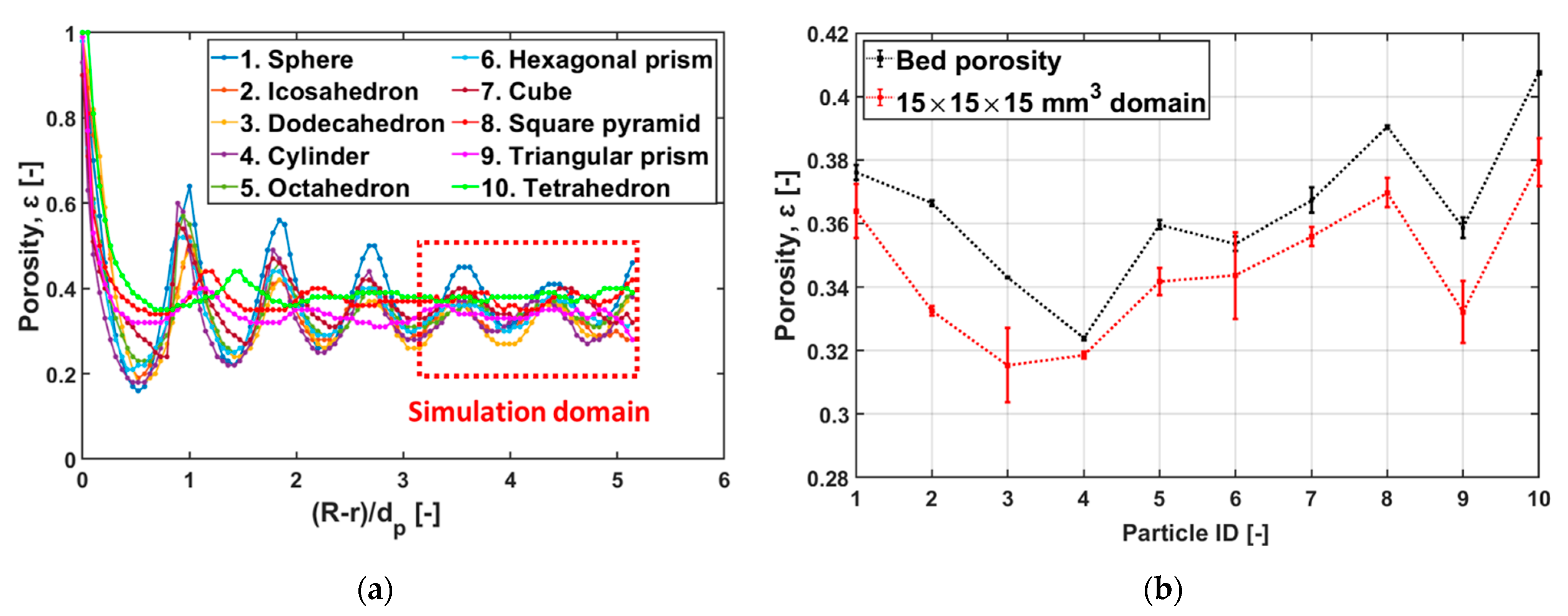
4.1. Packing Results

The particle packing results were compared using the porosities of the bed. The overall bed porosity and porosity profiles were only obtained for the height of 100 mm from the bottom of beds, since the major variation of porosity is on the top of the bed, discussed in [49]. This was performed to eliminate the effect of loose packing at the top of the bed, which could affect the results. Figure 3a provides the radial distribution of the porosity from the wall to the center of the cylinder. A drastic variation is observed at the cylinder wall for all particle shapes. It is followed by the strong oscillation of porosity for higher sphericity shapes, i.e., from the sphere to the octahedron ($\varphi$= 1 − 0.876). Oscillations rapidly fade away for particles with lower sphericity and a lower number of faces, like the tetrahedron and the triangular prism. Due to the long edges and lower sphericity of these particles, the particle orientations randomize right after particles adjacent to the cylinder wall. In many previous studies, it was seen that the wall effect for spherical particles disappears at around $D/d_p$ = 10 [61], in our case, we used a setup with $D/d_p$ = 10.48. Despite this, we can see some effect of the wall on the overall porosity of the bed. Therefore, to remove this effect from further calculations and simulations, the inner region—which is the simulation domain (red dotted lines)—was considered, as shown in Figure 3a. Henceforth, for further analysis and comparison, the simulation domain of 15 × 15 × 15 mm³ was investigated. Figure 3b provides the average bed and domain porosities obtained from three different realizations with respect to different particle shapes, denoted by particle IDs. The domain porosities without the wall, top, and bottom effects were smaller than the overall bed porosities. For further study, these average domain values were considered.

Figure 4 shows a comparison of the relation of different shape parameters with the porosities of the domain. The porosity deviations for different realizations are mentioned in

Table 2. Results of $\epsilon$, $\epsilon /\tau$, and $\tau$ for different particle shapes and their deviation among three realizations.

Particle ID	Particle Type	$\mathit{\epsilon }$	$\mathit{\epsilon }/\mathit{\tau }$	$\mathit{\tau }$
1	Sphere	0.364 ± 0.0084	0.248 ± 0.0062	1.470 ± 0.0105
2	Icosahedron	0.333 ± 0.0016	0.197 ± 0.0123	1.689 ± 0.0115
3	Dodecahedron	0.315 ± 0.0117	0.182 ± 0.0067	1.731 ± 0.1417
4	Cylinder	0.319 ± 0.0011	0.179 ± 0.0074	1.777 ± 0.0597
5	Octahedron	0.342 ± 0.0044	0.191 ± 0.0064	1.791 ± 0.0292
6	Hexagonal prism	0.344 ± 0.0135	0.194 ± 0.0080	1.769 ± 0.0129
7	Cube	0.356 ± 0.0030	0.194 ± 0.0049	1.836 ± 0.1276
8	Square pyramid	0.370 ± 0.0046	0.196 ± 0.0055	1.882 ± 0.0359
9	Triangular prism	0.332 ± 0.0075	0.206 ± 0.0116	1.838 ± 0.0465
10	Tetrahedron	0.379 ± 0.0098	0.180 ± 0.0009	1.848 ± 0.0296

and are not significant. The general trend in Figure 4a is that of porosity decreasing with increasing sphericity. However, this trend is weak in total because it is broken and inverted at very high sphericity (sphere [particle ID 1] and icosahedron [particle ID 2]). This may be explained by the smaller contact area or rather point contacts between the particles which result in larger void spaces adjacent to the contacts. Additionally, triangular prisms (particle ID 9) behave as an outliner and have lower porosity at the same sphericity compared with pyramids (particle ID 8). Large face contact may be the reason for this behavior, though not fully understood. Other 3D particle shape parameters, namely the number of faces, edges, and vertices, have a similar influence, with porosity decreasing with increasing parameter values (though, again, the trend is coarse and accompanied by outliners). These parameters are directly correlated, which is discussed in Section 4.4. In all three graphs (Figure 4b–d), the values for the sphere and the cylinder should not be overestimated, this is because the definition of the number of faces, edges, and vertices for those two particle shapes is arguable.

4.2. Thermal Results

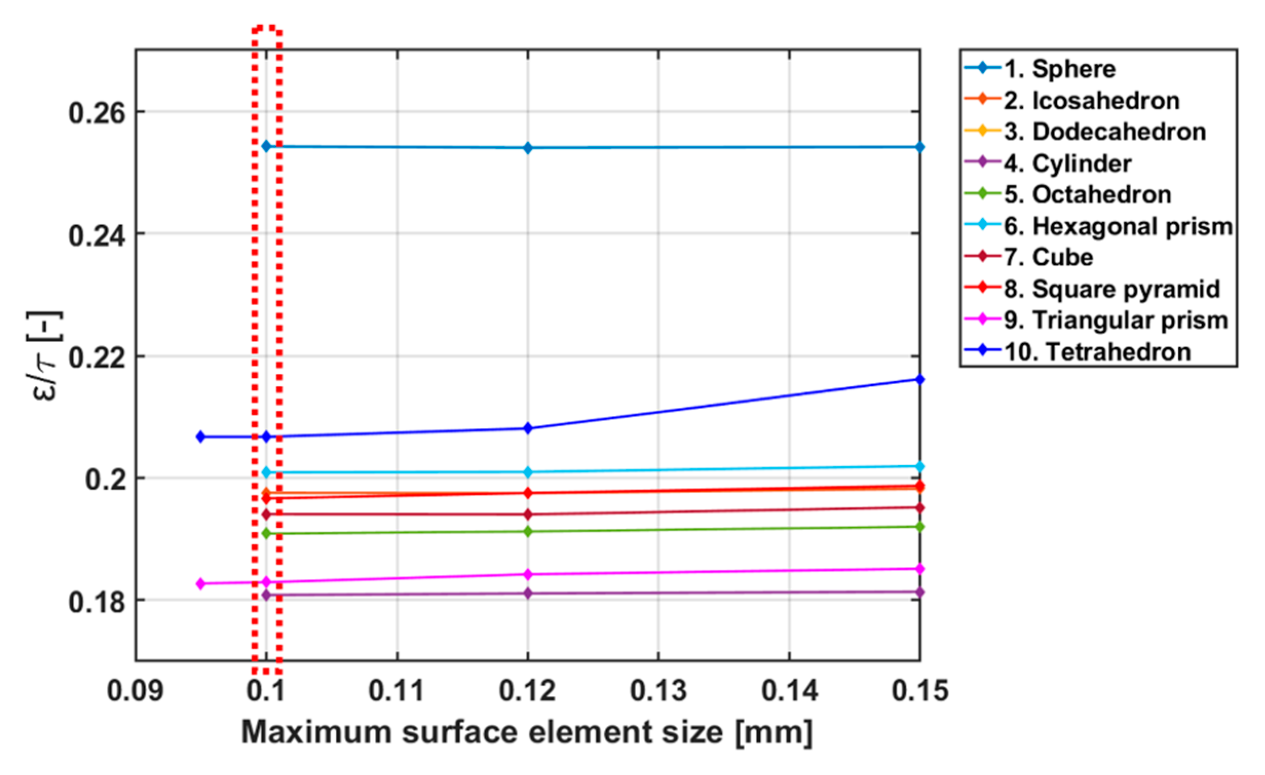
4.2.1. Mesh Independence Study for All Shapes

Mesh independence studies were conducted for all particle shapes with the same domain of size 15 × 15 × 15 mm³, as illustrated in Figure 2. The mesh sizing was based on the interface between the solid and gas phase, on which an unstructured octree mesh with a tetrahedral shape was placed. This interface mesh was then expanded to a volume mesh. Consequently, the maximum interface cell size is of importance for the ability of the simulation to resolve gaps between particles. This cell size varied from 0.09 to 0.15 mm for the study. This study was performed in the x-direction for all shapes, refer to Figure 2. The effective thermal conductivity with non-conducting particles, $k_{bed}(k_p\to 0)$, which is equivalent to $\epsilon /\tau$ (Equation (1)), is calculated using the heat flux obtained from simulations. The results of the study are depicted in Figure 5, where it is seen that the results are independent from the mesh for a maximal surface cell size of 0.1 mm, which is 2.6% of $d_p$. The change in $k_{bed}(k_p\to 0)$ was negligible from either cell size of 0.12 mm or at 0.1 mm. This was observed for all of the particle shapes; hence, 0.1 mm surface cell size was used for the simulations for every realization and also in the y-direction (the other lateral direction perpendicular to x). As mentioned, an average of three realizations in two directions for each shape is considered for further evaluation.

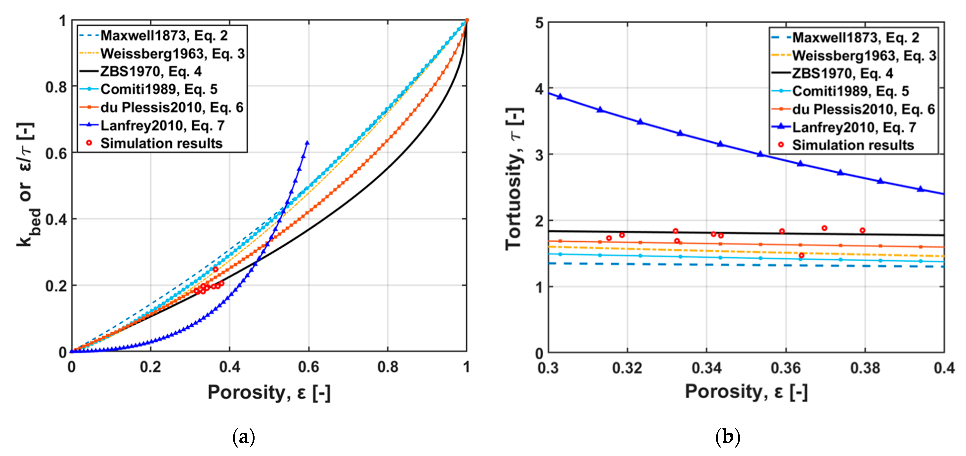
4.2.2. Comparison of Results with Old Models

The average values of bed conductivity and tortuosity obtained from the thermal simulation are plotted in Figure 6 with the old models previously explained. As mentioned in Section 2, all the old models, except for the Lanfrey model [46] and potentially also the Comiti model [39], are described with functions of only porosity. In our simulations, the range of porosities was relatively small, from 0.31 to 0.38 for all considered particle shapes. Variation of thermal diffusion in this porosity range was not so drastic; tortuosity was around 1.4 to 1.9, spherical particles being the outliner of the trend. When comparing models, the ZBS model (Equation (4)) has good agreement as observed in Figure 6a,b. The other model close to the simulation results was the du Plessis model [41] (Equation (6)) although they considered an isotropic staggered system for prediction, whereas in our simulations we had local anisotropy. The Comiti model uses an adjustable parameter ($C$ = 0.63 or 0.41, for cubes and spheres, respectively) to define the pore structure for different shapes. The values shown in Figure 6 are better described when using the Comiti model with $C$ = 0.63 for cubes. In Figure 6, the Lanfrey model [46] has been used with $\varphi$ = 0.806, also for cubes. Sphericity can be considered in this model, but the values of tortuosity obtained are much higher than our simulation results for cubes as well as for the other investigated particle shapes. This means that predictions by this model are highly exaggerating the tortuosity. Lanfrey et al. [46] only used a relation of bed porosity with sphericity for their model development, experimental values on diffusion were not available during their work. Additionally, the sphericities ($\varphi$ = 0–0.55) for determining their model were on the opposite side of the spectrum investigated in our work ($\varphi$ = 0.671–1), which is a possible reason for these differences.

As shown in Figure 7, the simulated residual conductivities seem close to the ZBS model equation. Significant deviation seems to be only present for the particle bed made of spheres. A detailed look at the values in Figure 7b reveals, however, a low R² value and systematic deviations of the data points along the ZBS curve, which is an indication of particles with different shape parameters affecting the values. These discrepancies or dependencies could be avoided by introducing further physical parameters into the ZBS model (Equation (4)). Respective modification of the ZBS model equation is discussed in Section 4.4. Prior to that, the dependence of the tortuosity on the particle shape needs to be studied in Section 4.3.

4.3. Effect of Particle Shape on Tortuosity

Figure 8 shows the tortuosity results for all shapes as a function of the sphericity of the particles. The major observation from these results is that tortuosity can be correlated to sphericity. The respective dependence is steepest for particle sphericity near 1. The results for packed beds of spheres were, indeed, completely off the tortuosity–porosity curves of porosity-based models. To quantify the obvious relation between tortuosity and sphericity, a rigorous curve-fitting procedure has been conducted on the simulated results to obtain a best-fitting curve based on the power law

$$\tau =-a{\varphi }^b+c.$$

(10)

The coefficients of the correlation were determined as $a$ = 0.382, $b$ = 12.36, and $c$ = 1.851, respectively. With these coefficients, Equation (10) yielded an R² value of 0.9672, which shows good agreement for the sphericity range used in this work, i.e., $\varphi$ = 0.65–1. However, it will be further refined, as be seen in Section 4.4.

In Figure 9, fitting curves of tortuosity are shown with other 3D particle shape parameters: number of faces, edges, and vertices. These fitting curves were obtained by excluding the spheres for the previously mentioned reason of disputable geometrical definitions that make these values outliers. Irrespective of this data, the trend of the results with all mentioned particle shape parameters was similar, which was also observed in the correlation matrix for the parameters shown in Figure 10, to be discussed in Section 4.4. The best curve fits derived employing power law fitting are also depicted in Figure 9. The results were found to be unusual, especially the coefficients. The coefficients are nearly identical, with the prefactor at around 2 and the exponent at around −0.056. This shows a strong inter-dependency between said geometrical parameters. Hence, it can be inferred that the tortuosity has the same relationship with the number of faces, the number of edges, and the number of vertices.

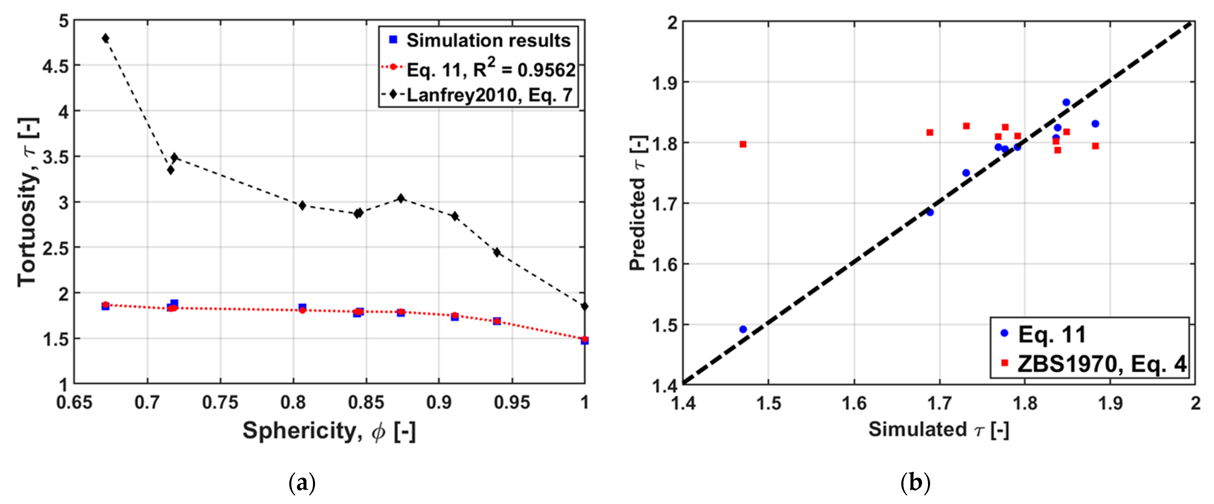
4.4. Modification of Tortuosity Equation—ZBS Model

A correlation matrix was created to understand the relation between parameters and their strength, as outlined in Figure 10. In this matrix, the correlation coefficients vary from −1 to 1, where negative represents an inverse correlation and positive value stands for a direct correlation. Values approaching zero indicate weakly related variables, whereas variables with a correlation coefficient close to one are strongly related. From the obtained matrix, the following observations can be deduced:

-

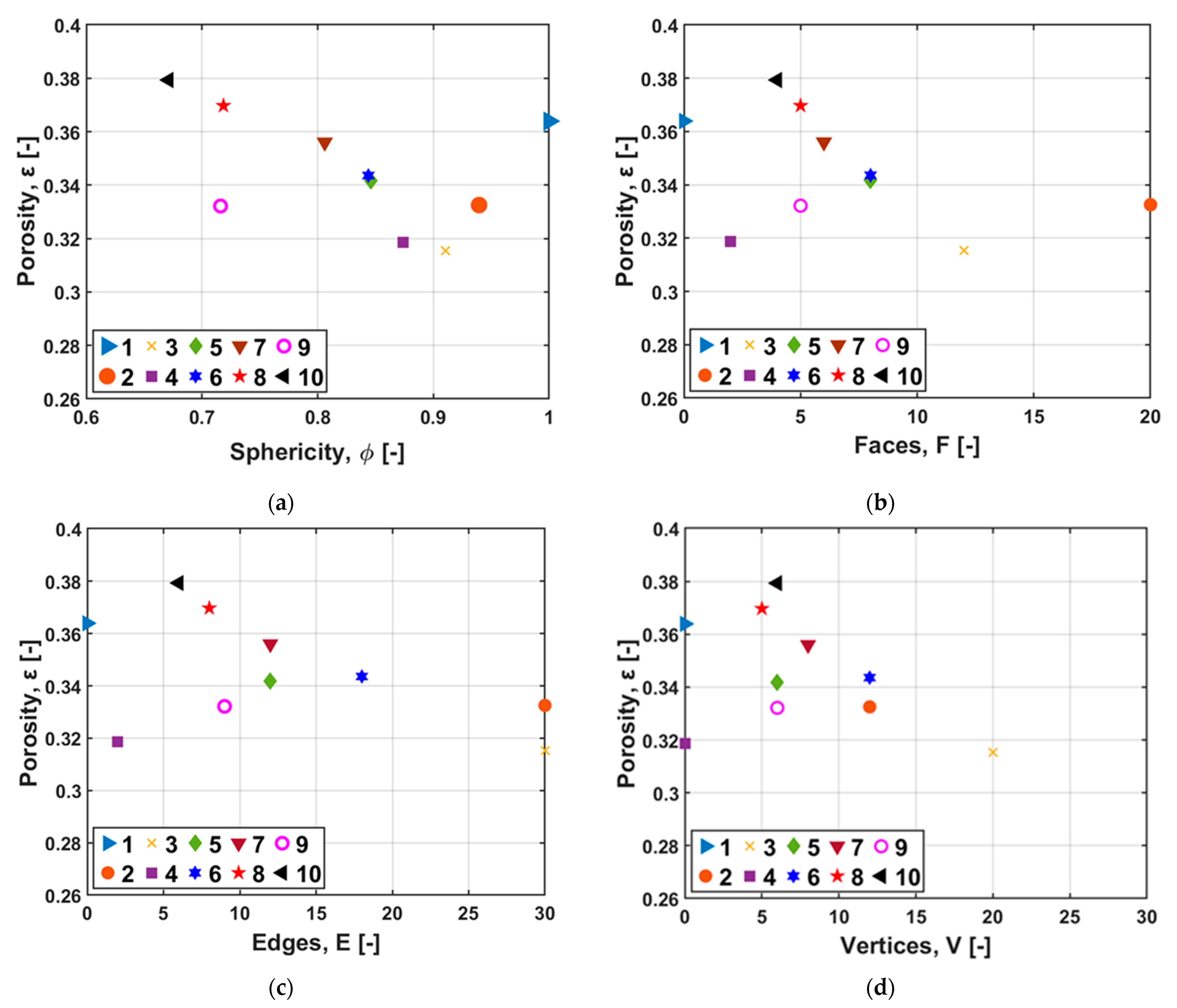
Porosity for our range of simulations was found to have a weak correlation to tortuosity, which is also observed in Figure 6b. Hence, the effect of other parameters is essential.

-

When considering $F$, $E$, and $V$, these variables are strongly interrelated to each other but weakly related to tortuosity. With porosity, they are moderately inversely related. This effect is detected in Figure 4, where higher porosities can be seen for lower values of $F$, $E$, and $V$.

-

As already indicated, sphericity dominates the correlation coefficient analysis for tortuosity, with those variables being proportional to each other.

Henceforth, for further expansion of the model, only the sphericity shape parameter was considered.

To introduce the sphericity in the tortuosity equation, the earlier derived fitted curve of Equation (11) with the ZBS model, Equation (4) was preferred for modification. Moreover, the ZBS model tortuosity was selected for being in better agreement with the simulated results than tortuosities from other models. A closer look into Equation (10) shows that the coefficient $c$ is close to the tortuosity of the ZBS model according to Equation (4). Therefore, the coefficient $c$ is replaced by ${{\tau }_{ZBS}}^n$, which is a function of porosity and where $n$ accounts for an increase of tortuosity with respect to simulated results. On the other hand, in the first term, which includes the sphericity, the coefficient $a$ is replaced by porosity, and the sphericity dependency is accounted by the exponent $m$ (replacing $b$). This term subtracts the effect of sphericity from the porosity-only relation (second term). The finally proposed tortuosity equation derived from Equation (10) is

$${\tau }_{Final}=-\epsilon {\varphi }^m+{{\tau }_{ZBS}}^n.$$

(11)

The same fitting method is again applied to the simulated results. The empirical constants of $m$ = 8.8788 and $n$ = 1.0534 were obtained. Using these coefficients, Equation (11) reproduces the data with R² = 0.9562, similar to Equation (10). The proposed model is compared with the old model from Lanfrey et al. [46] in Figure 11a. This model had a sphericity relation with tortuosity, but it is completely off the present simulations. Figure 11b demonstrates the accuracy of the proposed model compared with simulation results and to the ZBS model without sphericity term. However, it should be noted that Equation (11) has been derived considering limited ranges of porosity and sphericity, $\epsilon$ = 0.3–0.4 and $\varphi$ = 0.65–1, respectively. In these ranges, sphericity has an at least equally strong influence as porosity. Large changes in porosity, however, may increase its influence compared with the influence of sphericity. Thus, this work should be regarded as a first step in deriving a universal model to predict tortuosity based on particle parameters. Adding more parameters, like aspect ratios and pore morphology, could provide a model usable for a wide range of porosity.

5. Conclusions and Outlook

In this article, we studied how particle shape can affect the pore morphology of random packings resulting in a change of tortuosity, the primary parameter to characterize mass transport in porous media. Different particle shapes with a sphericity range of 0.671–1 were studied. The bed structures were created using rigid body simulation in the software Blender, from which domains for numerical simulations were considered without wall effect. Residual effective thermal conductivities or diffusivities were investigated using thermal simulations considering a non-conducting solid phase. Tortuosities were calculated and compared with different porosity-based models; the ZBS model [47] obtained from a large set of experiments was closest compared with other models. However, even this model was found to have some deviation from simulation data, caused by the influence of particle shape.

The attained tortuosity had a stronger relation to sphericity than to the number of faces, edges, and vertices when analyzed by the means of a correlation matrix. The number of faces, edges, and vertices had an almost identical effect on the tortuosity and dominant interdependency, which was interesting and somehow unusual. Hence, a new model was proposed by only introducing sphericity into the ZBS model. The proposed model was established by subtracting a new tortuosity term with porosity and sphericity from the ZBS model tortuosity, corresponding to the equation ${\tau }_{Final}=-\epsilon {\varphi }^m+{{\tau }_{ZBS}}^n$. The model exhibits very good results in the higher sphericity range and porosity of 0.3–0.4. Future improvements may use particles with different aspect ratios and non-regular shapes in order to widen the range of model applicability in regard to sphericity. Additionally, other packing methods may be considered to cover a broader range of porosity. Such results would help to further generalize the model for use in various applications that involve the conductance of particle systems.

References

1. Sharma, R.K.; Cresswell, D.L.; Newson, E.J. Effective Diffusion Coefficients and Tortuosity Factors for Commercial Catalysts. Ind. Eng. Chem. Res. 1991, 30, 1428–1433. [Google Scholar] [CrossRef]
2. Das, S.; Deen, N.G.; Kuipers, J.A.M. Multiscale Modeling of Fixed-Bed Reactors with Porous (Open-Cell Foam) Non-Spherical Particles: Hydrodynamics. Chem. Eng. J. 2018, 334, 741–759. [Google Scholar] [CrossRef]
3. Welsh, Z.G.; Khan, M.I.H.; Karim, M.A. Multiscale Modeling for Food Drying: A Homogenized Diffusion Approach. J. Food Eng. 2021, 292, 110252. [Google Scholar] [CrossRef]
4. Lammens, J.; Goudarzi, N.M.; Leys, L.; Nuytten, G.; van Bockstal, P.-J.; Vervaet, C.; Boone, M.N.; de Beer, T. Spin Freezing and its Impact on Pore Size, Tortuosity and Solid State. Pharmaceutics 2021, 13, 2126. [Google Scholar] [CrossRef]
5. Muhammed, N.S.; Haq, B.; Al Shehri, D.; Al-Ahmed, A.; Rahman, M.M.; Zaman, E. A Review on Underground Hydrogen Storage: Insight into Geological Sites, Influencing Factors and Future Outlook. Energy Rep. 2022, 8, 461–499. [Google Scholar] [CrossRef]
6. Boudreau, B.P.; Meysman, F.J.R. Predicted Tortuosity of Muds. Geology 2006, 34, 693. [Google Scholar] [CrossRef]
7. Peng, S.; Marone, F.; Dultz, S. Resolution Effect in X-Ray Microcomputed Tomography Imaging and Small Pore’s Contribution to Permeability for a Berea Sandstone. J. Hydrol. 2014, 510, 403–411. [Google Scholar] [CrossRef]
8. del Castillo, L.F.; Hernández, S.I.; Compañ, V. Obtaining the Tortuosity Factor as a Function of Crystallinity in Polyethylene Membranes; Maciel-Cerda, A., Ed.; Springer: Cham, Switzerland, 2017; pp. 77–86. [Google Scholar] [CrossRef]
9. Maerki, M.; Wehrli, B.; Dinkel, C.; Müller, B. The Influence of Tortuosity on Molecular Diffusion in Freshwater Sediments of High Porosity. Geochim. Cosmochim. Acta 2004, 68, 1519–1528. [Google Scholar] [CrossRef]
10. Tjaden, B.; Brett, D.J.L.; Shearing, P.R. Tortuosity in Electrochemical Devices: A Review of Calculation Approaches. Int. Mater. Rev. 2018, 63, 47–67. [Google Scholar] [CrossRef]
11. Lee, J.K.; Bazylak, A. Optimizing Porous Transport Layer Design Parameters via Stochastic Pore Network Modelling: Reactant Transport and Interfacial Contact Considerations. J. Electrochem. Soc. 2020, 167, 013541. [Google Scholar] [CrossRef]
12. Espinoza, M.; Andersson, M.; Yuan, J.; Sundén, B. Compress Effects on Porosity, Gas-Phase Tortuosity, and Gas Permeability in a Simulated PEM Gas Diffusion Layer. Int. J. Energy Res. 2015, 39, 1528–1536. [Google Scholar] [CrossRef]
13. Ostadi, H.; Rama, P.; Liu, Y.; Chen, R.; Zhang, X.X.; Jiang, K. 3D Reconstruction of a Gas Diffusion Layer and a Microporous Layer. J. Memb. Sci. 2010, 351, 69–74. [Google Scholar] [CrossRef] [Green Version]
14. Usseglio-Viretta, F.L.E.; Finegan, D.P.; Colclasure, A.; Heenan, T.M.M.; Abraham, D.; Shearing, P.; Smith, K. Quantitative Relationships Between Pore Tortuosity, Pore Topology, and Solid Particle Morphology Using a Novel Discrete Particle Size Algorithm. J. Electrochem. Soc. 2020, 167, 100513. [Google Scholar] [CrossRef]
15. Cooper, S.J.; Eastwood, D.S.; Gelb, J.; Damblanc, G.; Brett, D.J.L.; Bradley, R.S.; Withers, P.J.; Lee, P.D.; Marquis, A.J.; Brandon, N.P.; et al. Image Based Modelling of Microstructural Heterogeneity in LiFePO 4 Electrodes for Li-Ion Batteries. J. Power Sources 2014, 247, 1033–1039. [Google Scholar] [CrossRef]
16. Ghanbarian, B.; Hunt, A.G.; Ewing, R.P.; Sahimi, M. Tortuosity in Porous Media: A Critical Review. Soil Sci. Soc. Am. J. 2013, 77, 1461. [Google Scholar] [CrossRef]
17. Fu, J.; Thomas, H.R.; Li, C. Tortuosity of Porous Media: Image Analysis and Physical Simulation. Earth-Science Rev. 2021, 212, 103439. [Google Scholar] [CrossRef]
18. Cooper, S.J.; Bertei, A.; Shearing, P.R.; Kilner, J.A.; Brandon, N.P. TauFactor: An Open-Source Application for Calculating Tortuosity Factors from Tomographic Data. SoftwareX 2016, 5, 203–210. [Google Scholar] [CrossRef]
19. Sobieski, W.; Matyka, M.; Gołembiewski, J.; Lipiński, S. The Path Tracking Method as an Alternative for Tortuosity Determination in Granular Beds. Granul. Matter 2018, 20, 72. [Google Scholar] [CrossRef] [Green Version]
20. Stenzel, O.; Pecho, O.; Holzer, L.; Neumann, M.; Schmidt, V. Predicting Effective Conductivities Based on Geometric Microstructure Characteristics. AIChE J. 2016, 62, 1834–1843. [Google Scholar] [CrossRef]
21. Pardo-Alonso, S.; Vicente, J.; Solórzano, E.; Rodriguez-Perez, M.Á.; Lehmhus, D. Geometrical Tortuosity 3D Calculations in Infiltrated Aluminium Cellular Materials. Procedia Mater. Sci. 2014, 4, 145–150. [Google Scholar] [CrossRef] [Green Version]
22. Al-Raoush, R.I.; Madhoun, I.T. TORT3D: A MATLAB Code to Compute Geometric Tortuosity from 3D Images of Unconsolidated Porous Media. Powder Technol. 2017, 320, 99–107. [Google Scholar] [CrossRef]
23. Carman, P.C. Fluid Flow through a Granular Bed. Trans. Inst. Chem. Eng. 1937, 75, 150–167. [Google Scholar] [CrossRef]
24. Kozeny, J. Ueber kapillare Leitung des Wassers im Boden. R. Acad. Sci. Vienna Proc. Cl. I 1927, 136, 271–306. [Google Scholar]
25. Matyka, M.; Khalili, A.; Koza, Z. Tortuosity-Porosity Relation in Porous Media Flow. Phys. Rev. E 2008, 78, 026306. [Google Scholar] [CrossRef] [Green Version]
26. Piller, M.; Schena, G.; Nolich, M.; Favretto, S.; Radaelli, F.; Rossi, E. Analysis of Hydraulic Permeability in Porous Media: From High Resolution X-Ray Tomography to Direct Numerical Simulation. Transp. Porous Media 2009, 80, 57–78. [Google Scholar] [CrossRef]
27. Luo, L.; Yu, B.; Cai, J.; Zeng, X. Numerical Simulation of Tortuosity for Fluid Flow in Two-Dimensional Pore Fractal Models of Porous Media. Fractals 2014, 22, 1450015. [Google Scholar] [CrossRef]
28. Jin, G.; Patzek, T.W.; Silin, D.B. Direct In Proceedings of the Prediction of the Absolute Permeability of Unconsolidated and Consolidated Reservoir Rock. SPE Annual Technical Conference and Exhibition Proceeding, Houston, TX, USA, 26 September 2004. [Google Scholar] [CrossRef]
29. Degruyter, W.; Burgisser, A.; Bachmann, O.; Malaspinas, O. Synchrotron X-ray Microtomography and Lattice Boltzmann Simulations of Gas Flow through Volcanic Pumices. Geosphere 2010, 6, 470–481. [Google Scholar] [CrossRef] [Green Version]
30. Ahmadi, M.M.; Mohammadi, S.; Hayati, A.N. Analytical Derivation of Tortuosity and Permeability of Monosized Spheres: A Volume Averaging Approach. Phys. Rev. E 2011, 83, 026312. [Google Scholar] [CrossRef] [Green Version]
31. Guo, P. Lower and Upper Bounds for Hydraulic Tortuosity of Porous Materials. Transp. Porous. Med. 2015, 109, 659–671. [Google Scholar] [CrossRef]
32. Saomoto, H.; Katagiri, J. Direct Comparison of Hydraulic Tortuosity and Electric Tortuosity Based on Finite Element Analysis. Theor. Appl. Mech. Lett. 2015, 5, 177–180. [Google Scholar] [CrossRef] [Green Version]
33. Brown, L.D.; Abdulaziz, R.; Tjaden, B.; Inman, D.; Brett, D.J.L.; Shearing, P.R. Investigating Microstructural Evolution during the Electroreduction of UO2 to U in LiCl-KCl Eutectic Using Focused Ion Beam Tomography. J. Nucl. Mater. 2016, 480, 355–361. [Google Scholar] [CrossRef] [Green Version]
34. Maxwell, J.C. Treatise on Electricity and Magnetism; Clarendon Press: London, UK, 1873. [Google Scholar]
35. Wakao, N.; Smith, J.M. Diffusion in Catalyst Pellets. Chem. Eng. Sci. 1962, 17, 825–834. [Google Scholar] [CrossRef]
36. Weissberg, H.L. Effective Diffusion Coefficient in Porous Media. J. Appl. Phys. 1963, 34, 2636–2639. [Google Scholar] [CrossRef]
37. Tsotsas, E.; Martin, H. Thermal Conductivity of Packed Beds: A Review. Chem. Eng. Process. 1987, 22, 19–37. [Google Scholar] [CrossRef]
38. Kim, J.H.; Ochoa, J.A.; Whitaker, S. Diffusion in Anisotropic Porous Media. Transp. Porous Media 1987, 2, 327–356. [Google Scholar] [CrossRef]
39. Comiti, J.; Renaud, M. A New Model for Determining Mean Structure Parameters of Fixed Beds from Pressure Drop Measurements: Application to Beds Packed with Parallelepipedal Particles. Chem. Eng. Sci. 1989, 44, 1539–1545. [Google Scholar] [CrossRef]
40. Boudreau, B.P. The Diffusive Tortuosity of Fine-Grained Unlithified Sediments. Geochim. Cosmochim. Acta 1996, 60, 3139–3142. [Google Scholar] [CrossRef]
41. du Plessis, E.; Woudberg, S.; Prieur du Plessis, J. Pore-Scale Modelling of Diffusion in Unconsolidated Porous Structures. Chem. Eng. Sci. 2010, 65, 2541–2551. [Google Scholar] [CrossRef]
42. Pisani, L. Simple Expression for the Tortuosity of Porous Media. Transp. Porous Media 2011, 88, 193–203. [Google Scholar] [CrossRef]
43. Currie, J.A. Gaseous Diffusion in Porous Media. Part 2: Dry Granular Materials. Br. J. Appl. Phys. 1960, 11, 318–324. [Google Scholar] [CrossRef]
44. Wyllie, M.R.J.; Spangler, M.B. Application of Electrical Resistivity Measurements to Problem of Fluid Flow in Porous Media. Am. Assoc. Pet. Geol. Bull. 1952, 36, 359–403. [Google Scholar] [CrossRef]
45. Dullien, F.A.L. Porous Media: Fluid Transport and Pore Structure; Elsevier: Amsterdam, The Netherlands, 1979. [Google Scholar]
46. Lanfrey, P.Y.; Kuzeljevic, Z.V.; Dudukovic, M.P. Tortuosity Model for Fixed Beds Randomly Packed with Identical Particles. Chem. Eng. Sci. 2010, 65, 1891–1896. [Google Scholar] [CrossRef]
47. Zehner, P.; Schlünder, E.U. Waermeleitfahigkeit von Schuettungen bei maessigen Temperaturen. Chemie Ing. Tech. 1970, 42, 933–941. [Google Scholar] [CrossRef]
48. Blender Foundation, Blender 2.90. Available online: https://www.blender.org/ (accessed on 31 August 2020).
49. Rodrigues, S.J.; Vorhauer-Huget, N.; Tsotsas, E. Effective Thermal Conductivity of Packed Beds Made of Cubical Particles. Int. J. Heat Mass Transf. 2022, 194, 122994. [Google Scholar] [CrossRef]
50. Bender, J.; Erleben, K.; Trinkle, J. Interactive Simulation of Rigid Body Dynamics in Computer Graphics. Comput. Graph. Forum 2014, 33, 246–270. [Google Scholar] [CrossRef]
51. Cundall, P.A.; Strack, O.D.L. A Discrete Numerical Model for Granular Assemblies. Géotechnique 1979, 29, 47–65. [Google Scholar] [CrossRef]
52. George, G.R.; Bockelmann, M.; Schmalhorst, L.; Beton, D.; Gerstle, A.; Lindermeir, A.; Wehinger, G.D. Influence of Foam Morphology on Flow and Heat Transport in a Random Packed Bed with Metallic Foam Pellets-An Investigation Using CFD. Materials. 2022, 15, 3754. [Google Scholar] [CrossRef]
53. Fernengel, J.; Weber, R.; Szesni, N.; Fischer, R.W.; Hinrichsen, O. Numerical Simulation of Pellet Shrinkage within Random Packed Beds. Ind. Eng. Chem. Res. 2021, 60, 6863–6867. [Google Scholar] [CrossRef]
54. Partopour, B.; Dixon, A.G. An Integrated Workflow for Resolved-Particle Packed Bed Models with Complex Particle Shapes. Powder Technol. 2017, 322, 258–272. [Google Scholar] [CrossRef]
55. Ambekar, A.S.; Mondal, S.; Buwa, V.V. Pore-Resolved Volume-of-Fluid Simulations of Two-Phase Flow in Porous Media: Pore-Scale Flow Mechanisms and Regime Map. Phys. Fluids 2021, 33, 102119. [Google Scholar] [CrossRef]
56. Tsotsas, E. Particle-Particle Heat Transfer in Thermal DEM: Three Competing Models and a New Equation. Int. J. Heat Mass Transf. 2019, 132, 939–943. [Google Scholar] [CrossRef]
57. You, E.; Sun, X.; Chen, F.; Shi, L.; Zhang, Z. An Improved Prediction Model for the Effective Thermal Conductivity of Compact Pebble Bed Reactors. Nucl. Eng. Des. 2017, 323, 95–102. [Google Scholar] [CrossRef]
58. Wang, S.; Xu, C.; Liu, W.; Liu, Z. Numerical Study on Heat Transfer Performance in Packed Bed. Energies 2019, 12, 414. [Google Scholar] [CrossRef] [Green Version]
59. Bu, S.; Wang, J.; Sun, W.; Ma, Z.; Zhang, L.; Pan, L. Numerical and Experimental Study of Stagnant Effective Thermal Conductivity of a Graphite Pebble Bed with High Solid to Fluid Thermal Conductivity Ratios. Appl. Therm. Eng. 2020, 164, 114511. [Google Scholar] [CrossRef]
60. Bu, S.; Chen, B.; Li, Z.; Jiang, J.; Chen, D. An Explicit Expression of Empirical Parameter in ZBS Model for Predicting Pebble Bed Effective Thermal Conductivity. Nucl. Eng. Des. 2021, 376, 111106. [Google Scholar] [CrossRef]
61. von Seckendorff, J.; Hinrichsen, O. Review on the Structure of Random Packed-Beds. Can. J. Chem. Eng. 2021, 99, S703–S733. [Google Scholar] [CrossRef]
Figure 1. 3D particle shapes considered in this work with shape properties.
Processes 11 00003 g001
Figure 2. (a) Blender simulation of bed filling with particle array of 250 particles and (b) completely packed bed. (c) The smaller cubical domain highlighted in red was selected for thermal simulations, it is illustrated here with hexagonal prisms.
Processes 11 00003 g002
Figure 3. Porosities for different particle shapes: (a) radial porosity profiles, red-dotted lines represent the domain considered for thermal simulations and (b) comparison of bed and simulation domain porosities.
Processes 11 00003 g003
Figure 4. Variation of porosity with particle shape parameters for respective particle IDs: (a) sphericity; (b) number of faces; (c) number of edges; and (d) number of vertices.
Processes 11 00003 g004
Figure 5. Mesh independence study; dotted red represents the region where results are independent of the mesh size for all particle shapes.
Processes 11 00003 g005
Figure 6. Comparison of simulated results with prediction models: Equation (2) [34]; Equation (3) [36]; Equation (4) [47]; Equation (5) [39] with C = 0.63 for cubes; Equation (7) [46] with ϕ = 0.806 for cubes; and Equation (6) [41]. (a) Effective residual thermal conductivity or effective diffusivity and (b) tortuosity.
Processes 11 00003 g006
Figure 7. (a) Comparison of residual conductivity results with the ZBS model, Equation (4). (b) Expanded region of interest shown in green lines in (a).
Processes 11 00003 g007
Figure 8. Comparison of bed tortuosity as a sphericity function; dotted line represents the correlation of simulation data according to Equation (10).
Processes 11 00003 g008
Figure 9. Effect of particle shape parameters on tortuosity with fitted curves: (a) number of faces; (b) number of edges; and (c) number of vertices.
Processes 11 00003 g009
Figure 10. Correlation matrix between various parameters, where red represents a strong correlation.
Processes 11 00003 g010
Figure 11. (a) Comparison of the change in tortuosity with sphericity according to the proposed model and the Lanfrey model and (b) comparison between simulated tortuosity values with ZBS predictions and with values predicted by the here developed model, according to Equation (11).
Processes 11 00003 g011