Optimization Method of Jet Pump Process Parameters and Experimental Study on Optimal Parameter Combinations

Abstract

The performance of jet pumps depends significantly on their structural and operational parameters. Current research primarily concentrates on theoretical models and laboratory tests, with limited experimental investigations and comprehensive reports concerning jet pump performance under various parameter combinations. In this study, we take a comprehensive approach, integrating both experimental and theoretical methods to assess jet pump performance under optimized process parameters and sand-flushing capabilities. The key findings of this study are as follows: While the characteristic and efficiency equations of jet pumps effectively describe the interaction of critical factors, including the area ratio, pressure ratio, flow rate ratio, and density, they unfortunately do not account for the influence of crucial structural factors, such as the nozzle throat distance, throat length, and diffuser length, on overall performance. Moreover, the parameter optimization technique based on the P-M curve has limitations and requires a tailored design and evaluation to consider the maximum suction capacity in practical engineering contexts. Notably, the nozzle throat distance significantly affects the jet pump suction capacity. Increasing the nozzle throat distance from 6 mm to 12 mm substantially enhances the suction capacity, albeit with a minor reduction in the lifting capacity. Extending the distance from 12 mm to 18 mm initially boosts the suction capacity, followed by a subsequent decline, along with a decrease in the lifting capacity. Interestingly, jet pumps effectively handle sand suction at relatively low pump pressures, creating negative-pressure conditions. As the pump pressure increases, the suction capacity remains relatively stable. However, the lifting capacity increases proportionally with the pump pressure, providing valuable theoretical and technical insights for practical jet pump applications. In summary, our study introduces a comprehensive approach to evaluate jet pumps by integrating experimental and theoretical methods. These insights highlight the intricate relationship between jet pump characteristics and operational parameters, offering essential knowledge for the efficient utilization of jet pumps in various applications.

1. Introduction

During the oil well production process, fluids subject the sand grains within the reservoir to erosion, resulting in the detachment of some sand grains that enter the wellbore along with the fluids. This phenomenon leads to the deposition of sand in the wellbore [1,2]. The impact of sand deposition within the wellbore on the oil recovery rate is primarily observed in two aspects. Firstly, the significant accumulation of sand deposits in the wellbore can lead to reservoir blockages, resulting in a reduction in the rate of oil production or even a complete cessation of production [3,4]. Secondly, the fine sand particles that enter the oil production equipment along with the oil can cause equipment wear [5,6], thereby affecting normal production processes.

Currently, two primary measures are employed to address sand production in oil wells [7]. The first is sand control, which employs artificial methods to prevent sand from entering the wellbore. The primary methods include mechanical sand control and chemical sand control [8]. However, due to the high clay and fine sand content in reservoirs, sand control techniques can potentially lead to the blockage of sand control devices. Jet pumps, serving as fluid transport machinery and mixing reaction devices that operate on the principle of momentum exchange between fluids [9,10,11], offer an effective solution for sand production in oil wells. They can efficiently mitigate the abrasive impact of fine sand in the produced fluid by using high-pressure jet pumps. Nonetheless, the internal flow dynamics of the jet pump are intricate, and during the wellbore cleaning and sand production processes, the mixing of solid–liquid two-phase fluids results in significant energy losses [12,13,14], consequently leading to a reduced energy transmission efficiency of the jet pump. This limitation has been a hindrance to the development of jet pumps for sand production.

The performance of jet pumps is significantly influenced by both structural parameters and operating parameters. Consequently, scholars from both domestic and international backgrounds have undertaken extensive research on these two factors. Eames and Kumar, for instance, conducted optimization studies on the nozzle area ratio and nozzle throat distance of jet pumps. Their experimental findings indicated that the optimal performance of liquid–gas jet pumps is achieved when the throat distance is set to 33 mm [15]. Additionally, other researchers have conducted experimental investigations to explore the relationship between the nozzle outlet diameter, nozzle throat distance, area ratio, and performance of liquid–gas jet pumps. These studies have served to validate the theoretical results initially proposed by Kumar, with the experimental outcomes aligning consistently with the theoretical analyses [16].

Fried S. J. et al. conducted experiments to assess the performance of non-circular nozzle liquid–gas jet pumps. Their findings revealed that circular nozzles require a lower operating pressure than non-circular ones. Furthermore, when comparing their respective areas, non-circular nozzles achieved a higher maximum flow rate than circular ones [17]. In a separate study, Falk et al. performed numerical simulations on liquid–gas jet pumps, varying the nozzle throat distance. Their observations yielded the following insights: When the nozzle throat distance remains constant, the pressure ratio of the pump exhibits an inverse relationship with the flow rate ratio. When keeping the flow rate ratio constant, the pump’s efficiency initially increases and subsequently decreases as the nozzle throat distance is extended. They determined that the nozzle throat distance, which corresponds to the optimal pump performance, is approximately 1.5 times the nozzle exit diameter. Considering potential numerical simulation errors, it is reasonable to consider nozzle throat distances resulting in a roughly 5% decrease in the highest efficiency as acceptable. This implies that nozzle throat distances ranging from 1.0 to 1.7 times the nozzle throat diameter offer relatively good pump performance [18,19,20].

Jun et al. [21] conducted a study using FLUENT to examine the fluid characteristics of liquid–gas jet pumps. This investigation delved into the impact of varying suction chamber lengths and suction pipe positions on the flow distribution within the jet pump. Surprisingly, both factors were found to have minimal influence on the pump’s suction performance. Furthermore, the study scrutinized throat geometry and concluded that a contraction angle ranging from 13.5° to 17.1° led to higher pump efficiency. It was also determined that the optimal diameter for the suction chamber should be 1.56–1.68 times the diameter of the jet pipe. Importantly, experimental validation substantiated the precision of the numerical simulation results. Li et al. [22] discovered a close relationship between the pressure ratio, flow ratio, and efficiency of liquid–gas jet pumps and the diameter of the suction chamber. They identified an optimal range of suction chamber diameters that allows the pump to maintain higher efficiency. Ji et al. [23] focused on researching and optimizing the suction characteristics of liquid–gas jet pumps, exploring the impact of various structural parameters, such as the nozzle throat distance and area ratio. Their investigation revealed that the optimal nozzle throat distance for enhanced performance was 1.5 times the nozzle throat distance, with an area ratio falling within the 4–7 range. Moreover, they found that, compared to cylindrical nozzles, orifice nozzles exhibited superior suction characteristics and mixing effects. Additionally, the structure, arrangement, and quantity of the nozzles significantly influenced the internal flow field distribution of the pump, consequently affecting its efficiency. Wibisono K [24] employed numerical simulation methods to analyze how the nozzle distance, throat and nozzle area ratio, and throat length impacted the suction performance of liquid–gas jet pumps. The study provided optimal ranges for these parameters to achieve the highest efficiency.

In summary, the performance of a jet pump is primarily influenced by its structural and operational parameters. Currently, research methods predominantly center on theoretical and numerical simulations, with limited emphasis on experimental studies. Moreover, there is a dearth of reported investigations into the jet pump’s performance under various parameter combinations. To address these gaps, this study employs a comprehensive approach that integrates theoretical derivation with an experimental analysis. First, it establishes an optimization method for the jet pump’s process parameters. Second, it assesses the pump’s performance across diverse parameter combinations. Finally, it conducts an analysis of the pump’s sand-carrying capacity under static hydraulic pressure conditions. These findings offer valuable theoretical and technical insights for the practical application of jet pumps in the field.

2. Optimization Method for Negative-Pressure Jetting (Jet Pump) Process Parameters

2.1. The Basic Characteristics and Parameters of a Jet Pump [22]

Under the condition where the hydraulic pressure of the power fluid flowing through the jet pump is p₁ and the flow rate is q₁, the power fluid is pumped through the nozzle with a flow area of A_j. In the well, the liquid has a pressure of p₃ and a flow rate of q₃, and it is accelerated and drawn into the throat tube. After the throat tube, the accelerating fluid and the drawn-in fluid continuously mix, resulting in a change in pressure to the discharge pressure p₂ and a change in the flow rate to q₂, ultimately lifting it to the surface, as shown in Figure 1.

(1)

Dimensionless pressure ratio P:

The dimensionless pressure ratio P is defined as the ratio of the increment in the formation fluid pressure (p₂ − p₃) to the reduction in the hydraulic pressure of the power fluid (p₁ − p₂).

$$P=\left(p_2-p_3\right)/\left(p_1-p_2\right)$$

(1)

where p₁ represents the inlet pressure of the power fluid entering into the pump, p₂ is the pump discharge pressure, and p₃ is the inlet pressure of the drawn-in fluid entering into the pump.

(2)

Dimensionless volume flow ratio M:

The flow rate ratio M is defined as the ratio of the volume flow rate of the formation fluid q₁ to the volume flow rate of the power fluid q₃.

$$M=q_3/q_1$$

(2)

In the characteristic equation of a jet pump, the volume flow rate ratio M, often referred to as the flow rate ratio, is commonly used.

2.2. Basic Characteristic Equation and Efficiency Equation of Jet Pumps

$$P=\frac{p_2-p_3}{p_1-p_2}=\frac{1-N}{M+N}$$

(3)

where

$$\begin{array}{l}N=(1+K_j)+(1+K_s){\rho }_r\frac{M^3{R}^2}{{(1-R)}^2}+(1+K_{td})(1+{\rho }_{r}M)R^2{(1+M)}^2\\ -\left[2R(1+M)(1+{\rho }_r\frac{M^{2}R}{1-R})\right]/\left[(1+K_j)-(1+K_s){\rho }_r\frac{M^2{R}^2}{{(1-R)}^2}\right]\end{array}$$

(4)

The commonly used friction loss coefficients are shown in

Table 1. Friction loss coefficient table.

Identifying People	${\mathit{K}}_{\mathit{s}}$	${\mathit{K}}_{\mathit{j}}$	${\mathit{K}}_{\mathit{t}}$	${\mathit{K}}_{\mathit{d}}$	${\mathit{K}}_{\mathit{t}\mathit{d}}$
Gosline and O’Brien	0	0.15	0.28	0.10	0.38
Petrie	0	0.03			0.20
Cunningham	0	0.10			0.30
Sanger	0.036	0.14	0.102	0.102
Sanger	0.008	0.09	0.098	0.102

.

The efficiency of the jet pump, denoted as E, is defined as the ratio of the energy obtained from the formation fluid, E_s, to the energy supplied by the power fluid, E_j, as follows:

$$E=\frac{E_S}{E_j}=\frac{q_3\left(p_2-p_3\right)}{q_1\left(p_1-p_2\right)}=P\cdot M$$

(5)

In Equation (5), it can be seen that the efficiency depends on the product of the dimensionless pressure ratio and the dimensionless volume flow rate ratio.

2.3. Process Parameter Optimization Design Method

Under ideal conditions, when the pump operates at peak efficiency, we can derive the optimal structural parameters using the jet pump characteristic equation. However, in real-world scenarios, variations in pressure losses occur at different pump pressures and flow rates. Consequently, the actual pressure ratio does not align with the ideal pressure ratio, leading to suboptimal pump efficiency. Increasing the pump pressure can boost the pump’s lifting capacity but reduces the lifting pressure ratio. As a result, the jet pump’s operational range extends beyond the point of optimum efficiency, resulting in wasted pumping energy at the surface pump.

This design method aims to achieve the optimal pump efficiency while satisfying the minimum lifting pressure ratio, calculating the optimal structural parameters for the jet pump. The calculation process is shown in Figure 2.

2.3.1. Calculation of the Minimum Lifting Pressure Ratio

Minimum Pressure Ratio Constraint: While operating the jet pump to lift sand-laden fluid from the well bottom to the surface, it is necessary to ensure that the jet pump attains a minimum lifting pressure ratio, even when it is solely tasked with returning the fluid to the surface.

The inlet pressure of the power fluid is denoted as P₁, and the power fluid enters through the central tube of the concentric tube. It overcomes the frictional resistance along the way, which can be represented as Equation (6):

$$P_1=P_0+\rho gH-\Delta P_1$$

(6)

In the equation, P₀ represents the surface pump pressure in MPa. g is the gravitational acceleration in m/s². H is the well depth in meters. ΔP₁ represents the frictional loss of the power fluid in MPa.

The sand-laden fluid entering the jet pump overcomes the effects of the liquid column gravity and the frictional resistance along the pipeline to return to the surface. From this, the minimum value of the outlet pressure P_2min can be determined using Equation (7):

$$P_{2\min }=\rho gH+\Delta P_2$$

(7)

where ΔP₂ represents the frictional loss of the returned fluid, specifically the frictional loss at the annular space, measured in MPa.

(1)

Loss of hydraulic pressure in the power fluid

If the power fluid enters from the central tube of the concentric tube, then we obtain Equation (8):

$$v_0=\frac{Q_0}{S}=\frac{4Q_0}{\pi D^2}$$

(8)

where v represents the velocity of the power fluid in m/s. Q represents the flow rate of the power fluid in m²/s. S represents the cross-sectional area of the pipeline in m². D represents the pipe diameter in meters.

The formula for calculating the Reynolds number is shown in Equation (9):

$$\mathrm{Re}=\frac{\rho vd}{{\mu }_0}$$

(9)

where μ represents the viscosity of the power fluid. When treating the power fluid as pure water, the viscosity of the power fluid is taken as the viscosity of the water, ${\mu }_0=1.0\times {10}^{-6}$ m²/s.

The calculation of frictional losses in the continuous oil tubing is divided into two parts: the straight section and the coiled section. The frictional loss of the power fluid is represented by Equation (10):

$$\Delta P_1=\Delta P_{ST}+\Delta P_{CT}$$

(10)

where ΔP_ST represents the frictional loss in the straight section in MPa. ΔP_CT represents the frictional loss in the coiled section in MPa.

Frictional loss in the straight section:

$$\Delta P_{ST}=\frac{1}{4}\left(f_{\mathrm{Blasius}}+f_{\mathrm{Drew}}+f_{\mathrm{Colebrook}}+f_{\mathrm{Chen}}\right)\frac{2\rho L{v}^2}{d_i}$$

(11)

Blasius model:

$$f_{Blasius}=\frac{0.0791}{{\mathrm{Re}}^{0.25}}$$

(12)

where f represents the dimensionless Darcy–Weisbach friction factor inside the pipe. Re represents the dimensionless Reynolds number.

Drew model:

$$f_{Drew}=0.0014+0.125{\mathrm{Re}}^{-0.32}$$

(13)

Colebrook model:

$$\frac{1}{\sqrt{f_{Colebrook}}}=-4\log \left(0.269\frac{\epsilon }{d_i}+\frac{1.255}{\mathrm{Re}\sqrt{f_{Colebrook}}}\right)$$

(14)

where ε represents the surface friction coefficient inside the oil tubing in meters (m). d_i represents the inner diameter of the oil tubing in meters (m).

Chen model:

$$\frac{1}{\sqrt{f_{Chen}}}=-4\log \left\{\frac{\epsilon }{3.7065d}-\frac{5.0452}{\mathrm{Re}}\log \left[\frac{1}{2.8257}{\left(\frac{\epsilon }{d}\right)}^{1.1098}+\frac{5.8506}{{\mathrm{Re}}^{0.8981}}\right]\right\}$$

(15)

The frictional loss in the coiled section:

$$\Delta P_{CT}=\frac{1}{3}\left(f_{\mathrm{White}}+f_{\mathrm{Ito}}+f_{\mathrm{Srinivasan}}\right)\frac{2\rho L{v}^2}{d_i}$$

(16)

The friction factor in the coiled section under turbulent flow conditions:

$$f_{CT}=f_{ST}+C\sqrt{\frac{r}{R}}$$

(17)

In the equation, f_CT represents the dimensionless Darcy–Weisbach friction factor in the coiled section of the continuous oil tubing under turbulent flow conditions. f_ST represents the dimensionless Darcy–Weisbach friction factor in the straight section of the continuous oil tubing under turbulent flow conditions. C represents the dimensionless empirical constant. There are three models represented in

Table 2. Values of each model constant C and their applicable ranges.

Model	C	Scope of Application
		r/R	Condition
White	0.012	0.00048–0.066	6000 < NRe < 100,000
Mishra and Gupta	0.0075	0.0289–0.15	4500 < NRe < 100,000
Correction to	0.0075	0.00154–0.0609	0.034 < NRe(r/R)2 < 300

.

For the Mishra and Gupta model, f_ST = 0.079/N_Re^0.25; for the other two models, f_ST = a/Re^b.

Srinivasan model:

$$f=\frac{0.084}{{\mathrm{Re}}^{0.2}}{\left(\frac{r}{R}\right)}^{0.1}$$

(18)

Under the same Reynolds number conditions, the White model and the Mishra and Gupta model exhibit the highest friction coefficients, followed by the Srinivasan model, while the modified Ito model shows the lowest friction coefficient. Consequently, for the calculations in this context, only the White model is utilized.

As demonstrated in the equation above, varying flow rates lead to different Reynolds numbers, consequently resulting in distinct Darcy–Weisbach friction factors for the straight section. The pressure loss fluctuates with changes in the flow rate. The Reynolds numbers for various operational scenarios are computed using (Equation (9)), and the four Darcy–Weisbach friction factors for the straight section are determined through (Equation (11)) to (Equation (14)). Subsequently, the friction factor for the straight section is derived from (Equation (10)). Similarly, the four Darcy–Weisbach friction factors for the coiled section are calculated using (Equations (16)–(19)), and the friction factor for the coiled section is extracted from (Equation (20)).

(2)

Flowback fluid pressure loss $\Delta P_2$

The flowback fluid is discharged from the annulus; then,

$$v_1=\frac{Q_1}{S}=\frac{4Q_{{}_1}}{\pi D^2}$$

(19)

where v₁ represents the velocity of the returned fluid in m/s. Q₁ represents the flow rate of the returned fluid in m²/s. S represents the annular space area in m². D represents the annular space diameter.

Reynolds number calculation formula:

$$\mathrm{Re}=\frac{\rho vd}{{\mu }_1}$$

(20)

where μ₁ represents the viscosity of the returned fluid, and it is assumed to be the viscosity of the returned fluid ${\mu }_0=1.0\times {10}^{-6}{\mathrm{m}}^2/\mathrm{s}$.

Friction loss coefficient:

$$f_{Drew}=0.0014+0.125{\mathrm{Re}}^{-0.32}$$

(21)

Flowback fluid pressure loss $\Delta P_2$:

$$\Delta P_2=\frac{2\rho L{v}^2}{d_i}$$

(22)

(3)

Minimum lifting pressure ratio $P_{\min }$

The pressure parameters P₁, P_2min, and P₃ of the jet pump can be calculated using the above calculations. The minimum lifting pressure ratio, just enough for returning, is represented as Equation (23):

$$P_{\min }=\left(P_{2\min }-P_3\right)/\left(P_1-P_{2\min }\right)$$

(23)

2.3.2. Optimal Parameter Calculation [24]

(1)

Ideal Pump Efficiency and Optimal Parameters

Based on the above jet pump basic characteristic equations, the pressure ratio P and pump efficiency E are both equations in terms of the flow rate M. By combining equations (Equations (3)–(5)), the pump efficiency equation for the jet pump can be derived as Equation (24):

$$E=\frac{\eta -\psi }{\xi (1+\mathrm{M})}\mathrm{M}$$

(24)

where $\xi =(1+K_{\mathrm{j}})+(1+K_{\mathrm{t}\mathrm{d}})R^2(1+{\rho }_{\mathrm{r}}M)(1+M)-2R(1+{\rho }_{\mathrm{r}}{M}^2\frac{R}{1-R})$; $\mathsf{\eta }=\left(1+K_{\mathrm{j}}\right)-\left(1+K_{\mathrm{s}}\right){\rho }_{\mathrm{r}}\frac{M^2{R}^2}{(1-R{)}^2}$.

In the design process, the optimal pump efficiency of the jet pump is taken as the goal. According to the solution method of the optimal value of the multivariate function, the optimal pump efficiency is solved as follows: $\partial E/\partial M=0$. We can find the maximum value of E. Thus, the ideal flow ratio under the condition of optimal pump efficiency can be obtained $M_{out}$:

$$M_{out}=\frac{\xi -\eta }{{\eta }^{\prime }\xi -\eta {\xi }^{\prime }}\xi$$

(25)

where ${\eta }^{\prime }=-2\left(1+K_{\mathrm{s}}\right){\rho }_{\mathrm{r}}M{\left(\frac{R}{1-R}\right)}^2,$ ${\xi }^{\prime }=(1+K_{\mathrm{t}\mathrm{d}})R^2(1+{\rho }_{\mathrm{r}}+2{\rho }_{\mathrm{r}}M)-4{\rho }_{\mathrm{r}}M\frac{R^2}{1-R}$.

The equation presented above (Equation (25)) represents the implicit expression for the flow rate ratio at optimal pump efficiency. The solution of this equation provides the flow rate ratio value corresponding to the optimal efficiency point across varying area ratio (R) conditions. Given that both the pressure ratio and pump efficiency are solely dependent on M, it is possible to calculate the optimal pressure ratio and pump efficiency for the jet pump in this scenario. These values can then be utilized to optimize various structural parameters of the jet pump, ensuring that it operates at peak efficiency.

By employing an interpolation method, we derived an efficiency envelope curve for the jet pump, illustrated in Figure 3. This figure reveals that each area ratio corresponds to its own efficiency curve, with each curve exhibiting a distinct maximum efficiency value. The efficiency envelope curve, represented as the fitted line for maximum efficiencies across various area ratios, identifies a clear maximum point, which signifies the optimal value for the jet pump across all area ratios. Utilizing the optimal flow rate ratio obtained from (Equation (25)) at the peak pump efficiency, we can calculate the optimal area ratio, subsequently allowing for the determination of the optimal pressure ratio. As Figure 3 demonstrates, through the application of interpolation and iterative methods, we ascertained the following optimal parameters for the jet pump: an optimal flow rate ratio of 1.071, an optimal pressure ratio of 0.373, a maximum pump efficiency of 39.95%, and an optimal area ratio of 0.280.

(2)

Optimal Parameters under Actual Operating Conditions

As shown in Figure 3, as the flow rate ratio of the jet pump increases, the efficiency envelope curve first increases and then decreases. With a constant pump pressure, the pressure ratio P₀ of the jet pump can be determined based on the minimum pressure ratio criterion. This, in turn, yields the actual flow rate ratio M₀. The design of optimal parameters for the jet pump under actual operating conditions can be categorized into two scenarios:

When the actual flow rate ratio M₀ is greater than the ideal flow rate ratio M_out, the ideal pump efficiency of the jet pump falls within the operational range. In this case, the displacement of the surface pump can be adjusted to achieve the optimal pump efficiency. Under these conditions, the design parameters for the jet pump can be set to the ideal structural parameters.

When the actual flow rate ratio M₀ is less than the ideal flow rate ratio M_out, the optimal pump efficiency of the jet pump corresponds to the value obtained from the efficiency envelope curve at the flow rate ratio M_o.

Based on the above, the jet pump efficiency E₁, optimal area ratio R₁, optimal flow rate ratio M₁, and optimal pressure ratio P₁ can be determined under actual operating conditions.

For example:

At a pump pressure of 50 MPa and a flow rate of 70 L/min, the minimum required lifting pressure ratio is 0.296. At this point, with an area ratio (R) of 0.1, it does not meet the minimum pressure ratio for negative-pressure sand removal. However, at R = 0.2, the jet pump’s efficiency exceeds the optimum level. As shown in the graph, when the pump pressure is maintained at 50 MPa and the pump displacement falls within the range of 60–100 L/min, the minimum required lifting pressure ratio for the jet pump remains below 0.373, allowing it to reach its theoretical maximum efficiency. Under these conditions, the structural design parameters for the jet pump can be established as follows: an optimal flow rate ratio of 1.071, an optimal pressure ratio of 0.373, a maximum pump efficiency of 39.95%, and an area ratio of 0.280 (refer to Figure 4 and Figure 5).

2.3.3. Structural Parameter Calculation [24,25]

Based on the previously calculated optimal flow rate ratio, pressure ratio, and area ratio for maximum pump efficiency, the calculation of the jet pump throat diameter, throat length, and nozzle diameter is performed.

(1)

Nozzle diameter:

$$d=\sqrt[4]{\frac{0.081{\rho }_{\mathrm{d}}{Q}^2}{{\mathrm{C}}^2 ({\mathrm{P}}_1-{\mathrm{P}}_3)}}$$

(26)

(2)

Throat diameter:

$$d_2=\sqrt{R·{\mathrm{d}}^2}$$

(27)

where d_s is the sand grain diameter, mm; a is the safety factor (in order to prevent particles from jamming the throat, the safety factor is 1.5 here).

(3)

Pipe length:

$${\mathrm{L}}_{\mathrm{k}}=\mathrm{n}{\mathrm{d}}_2=\left(\frac{0.2251}{R}+5.6037\right)d_2$$

(28)

Here, d₂ is the throat diameter, mm; R = d₂²/d² is the area ratio.

(4)

Laryngeal mouth distance:

$${\mathrm{L}}_{\mathrm{c}}=1\times {\mathrm{d}}_2$$

(29)

Here, d₂ is the throat diameter, mm.

From Equation (29), the nozzle diameter of the jet pump can be calculated under different pump pressures and displacements to maximize the jet pump efficiency.

3. Experimental Setup and Procedures

3.1. Experimental Apparatus

Figure 6 depicts the experimental setup for the wellbore simulation test. The research team machined a prototype jet pump based on the preliminary theoretical calculations for the relevant operating conditions, determining the tool’s structural parameters. In this experiment, a jet pump nozzle with a 2.5 mm diameter was utilized, while throat diameters of 3.5 mm and 4 mm were employed. Various nozzle distances of 6 mm, 12 mm, 15 mm, and 18 mm were tested. Throughout the experiment, the alteration of the jet pump area ratios was achieved by replacing the throat diameter. Different configurations, including nozzle distances, area ratios, and the jet pump’s suction capacity and efficiency under varying pump pressures, were examined, taking into account the presence or absence of confining pressure conditions.

3.2. Experimental Procedures

(1)

Prototype Installation: Following the optimization of the experimental results for the jet pump parameters, a parameter combination for the power nozzle, throat, and nozzle throat distance, suitable for general operating conditions, was chosen. In the experiment, 1 mm thick metal gaskets were employed to adjust the nozzle throat distance. These selected jet pump components were then installed onto the negative-pressure sand-flushing tool. Subsequently, a forward nozzle was chosen and installed based on the actual experimental displacement limit.

(2)

Tool and Pipeline Installation Preparation: The tool was connected to the high-pressure and return pipelines using dedicated connectors. The tool was securely fastened with suspension ropes and lowered into the simulated wellbore.

(3)

Wellbore Preparation: Quartz sand (30–50 mesh) was prepared and introduced into the bottom of the simulated wellbore, creating a bed with a height of approximately 2 m. Clear water was injected into the wellbore through the water supply pipeline to maintain a consistent liquid level. This step prevents air suction and maintains suction efficiency during prototype operation. The return pipeline was connected to the recovery tank.

(4)

Data Line Connection: Connectors for pressure gauges and flowmeters were installed at appropriate positions on the pumping pipeline. The other ends of the pressure gauges and flowmeters were linked to a junction box, which was in turn connected to the computer host. This setup facilitated the real-time monitoring and recording of pressure and flow changes on the computer screen.

(5)

Fixation of High-Pressure Pipeline: For safety reasons, flat lifting straps were securely installed and locked onto the jet pump pipeline to prevent the risk of fluid spray caused by unstable pipeline connections.

(6)

Pump Startup: The pump was gradually initiated to reach the designed test displacement. Once the flow rate and pressure stabilized, the increase in the pump displacement was continued until the pressure reached 25 MPa (a typical design value). The corresponding flow rate and pressure were recorded, the decrease in the liquid level in the wellbore was observed, and the water supply pipeline displacement was adjusted to maintain a stable liquid level.

(7)

Ground personnel responsible for the hoist confirmed the stability of the operating parameters before the tool was lowered. When the tool was approximately 30 cm above the sand surface, the bed became fluidized and suspended. Changes in the operating parameters were observed, and the lowering of the tool was continued slowly to avoid potential issues, such as the blockage of internal flow passages due to an excessively thick slurry caused by a rapid descent.

To assess the tool’s downward insertion velocity adequacy, we conducted an observation of sand production within the return flow pipeline. Sand that exited through the return outlet was filtered, collected, and subsequently measured. The experimental parameters are presented in

Table 3. Experimental parameters for jet pump testing.

Experimental Group	Dimensions of the Power Nozzle/mm	Diameter of the Throat/mm	Nozzle Throat Distance/mm	Length of the Throat/mm	Dimensions of the Diffuser/mm	Pump Pressure/MPa	Throttling Pressure/MPa
1–1	2.2	3	5	30	30	5–50	0–25
1–2		3	8	30	30	5–50	0–25
1–3		3	11	30	30	5–50	0–25
1–4	2.2	3.5	5	30	30	5–50	0–25
1–5		3.5	8	30	30	5–50	0–25
1–6		3.5	11	30	30	5–50	0–25
1–7	2.2	4	5	30	30	5–50	0–25
1–8		4	8	30	30	5–50	0–25
1–9		4	11	30	30	5–50	0–25

.

3.3. Experimental Results and Analysis

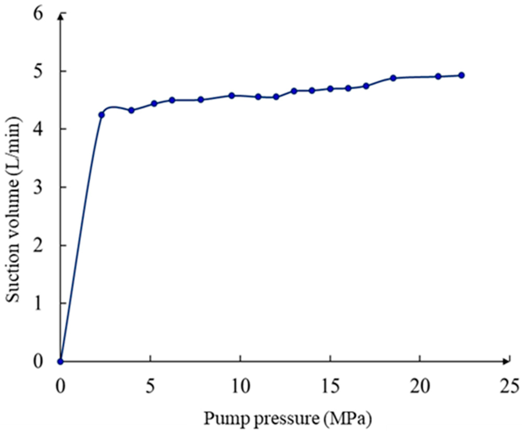
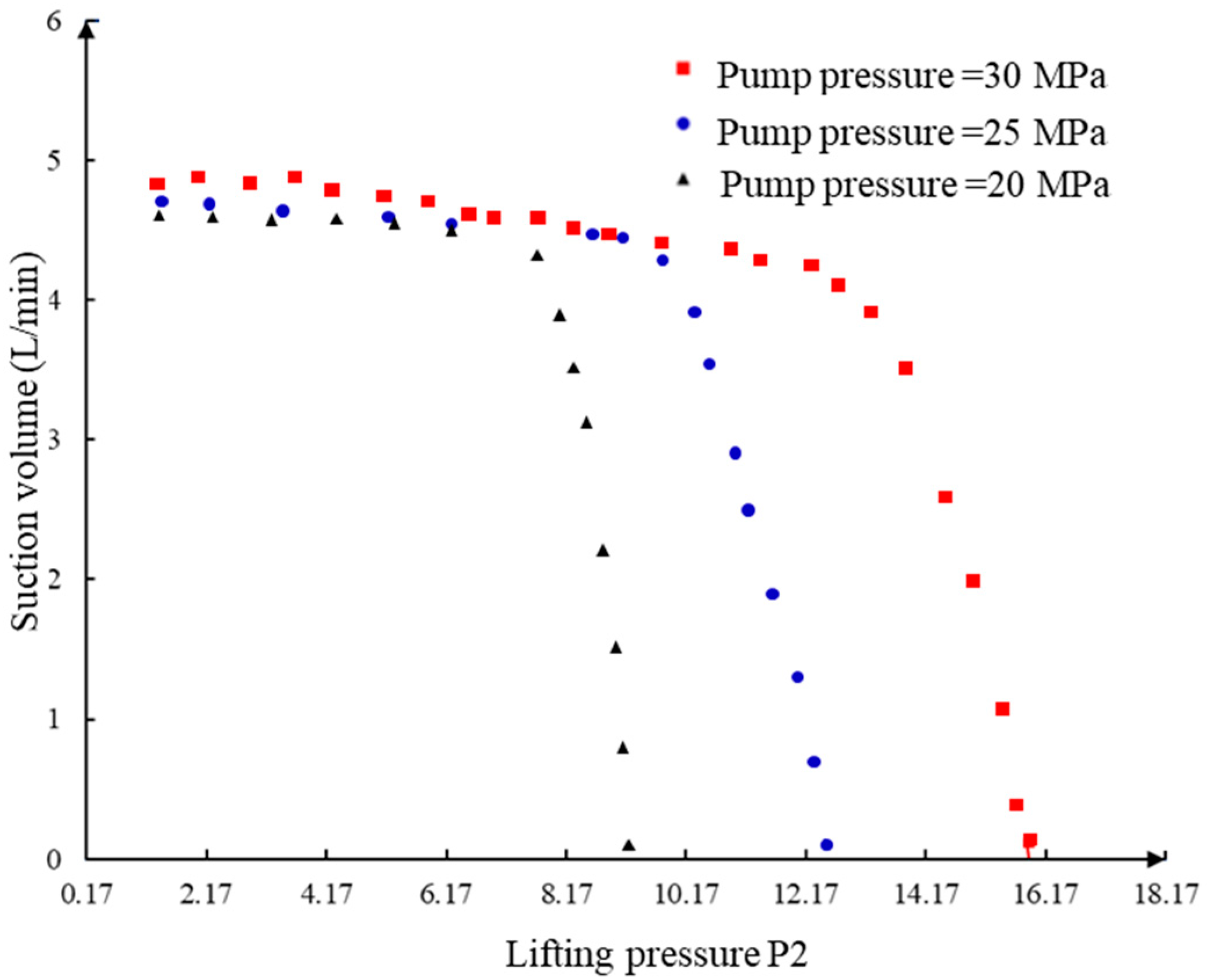
3.3.1. The Influence of Pump Pressure on the Performance of Jet Pumps

Figure 7 illustrates how the pump pressure affects the suction capacity of a jet pump. In the operational process, where the nozzle has a diameter of 2.2 mm, the throat diameter is 3.5 mm, and the nozzle distance is 6 mm, we observe a gradual increase in the jet pump’s suction capacity as the pump pressure rises. However, a turning point emerges at a pump pressure of 4.5 MPa. Beyond this threshold, further increases in the pump pressure do not result in a higher suction capacity of the jet pump.

Figure 8 illustrates the performance of the jet pump operating with specific dimensions: a 2.2 mm nozzle diameter, a 3.5 mm throat diameter, and a nozzle-to-throat distance of 6 mm. The suction capacity of the jet pump remains consistently stable as the lifting pressure increases. However, a noteworthy drop in the suction capacity becomes evident at a certain pressure threshold. Specifically, at pump pressures of 20 MPa, 25 MPa, and 30 MPa, we observe an initial decline in the suction capacity under lower pump pressure conditions. With an increase in the pump pressure, the lifting pressure $P_2$ of the jet flow exhibits a clear rise, while the maximum suction capacity of the jet pump remains essentially unchanged. This indicates that, under these specific structural parameters, increasing the pump pressure can significantly enhance the lifting pressure, allowing the gravel at the bottom of the well to be discharged to a higher ground level, thereby increasing the jet pump’s backflow capacity. However, the suction capacity of the jet pump does not increase with the increase in the pump pressure, indicating the inability to augment the suction capability of the jet pump. At a pump pressure of 30 MPa, the maximum suction capacity of the jet pump is approximately 4.9 L/min, with a lifting pressure of approximately 16 MPa.

As shown in Figure 9, the pressure ratio of the jet pump decreases with an increase in the flow rate ratio of the jet pump. When the nozzle diameter of the jet pump is 2.2 mm, the throat diameter is 3.5 mm, and the nozzle distance is 6 mm, at pump pressures of 20 MPa, 25 MPa, and 30 MPa, the pressure ratio of the jet pump exhibits a decreasing trend, which is particularly pronounced at higher pump pressures.

In Figure 10, the suction efficiency of the jet pump exhibits a trend of initially increasing and then decreasing with an increase in the flow rate ratio. Specifically, when the jet pump has a nozzle diameter of 2.2 mm, a throat diameter of 3.5 mm, and a nozzle distance of 6 mm and operates at pump pressures of 20 MPa, 25 MPa, and 30 MPa, we observe that the maximum efficiency of the jet pump initially rises and then declines as the flow rate ratio increases. Notably, the peak efficiency is achieved at a pump pressure of 25 MPa, surpassing the other two pressures. This peak efficiency reaches approximately 7%.

3.3.2. The Influence of Nozzle Throat Distance on the Performance of Jet Pumps

In Figure 11, we observe that, with a nozzle diameter of 2.2 mm, throat diameter of 4 mm, and pump pressure of 30 MPa, the jet pump’s maximum suction capacity increases as the nozzle throat distance extends from 12 mm to 15 mm. Beyond this point, from 15 mm to 18 mm, there is a slight additional increase in the maximum suction capacity. Notably, as the nozzle throat distance extends from 15 mm to 18 mm, there is a corresponding decrease in the maximum lift pressure ratio.

In Figure 12, we can observe that, as the pumping pressure reaches 30 MPa, the maximum flow rate of the jet pump rises as the nozzle distance increases. Simultaneously, the maximum lift pressure ratio, represented as ‘M,’ maintains a relatively constant value. Figure 12 also illustrates the efficiency behavior of the jet pump. Initially, it increases as the nozzle distance extends, reaching its peak at 15 mm, after which it starts to decrease.

In Figure 13, for a shallower well with a jet pump nozzle diameter of 2.2 mm and a pump pressure of 30 MPa, increasing the nozzle throat distance from 12 mm to 18 mm results in the maximum suction capacity. However, for deeper wells, to maintain the jet pump’s maximum lifting capacity and operational efficiency, a nozzle throat distance of 15 mm is recommended.

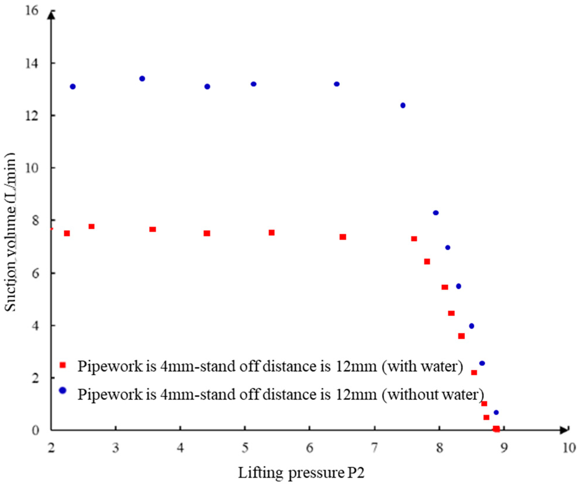
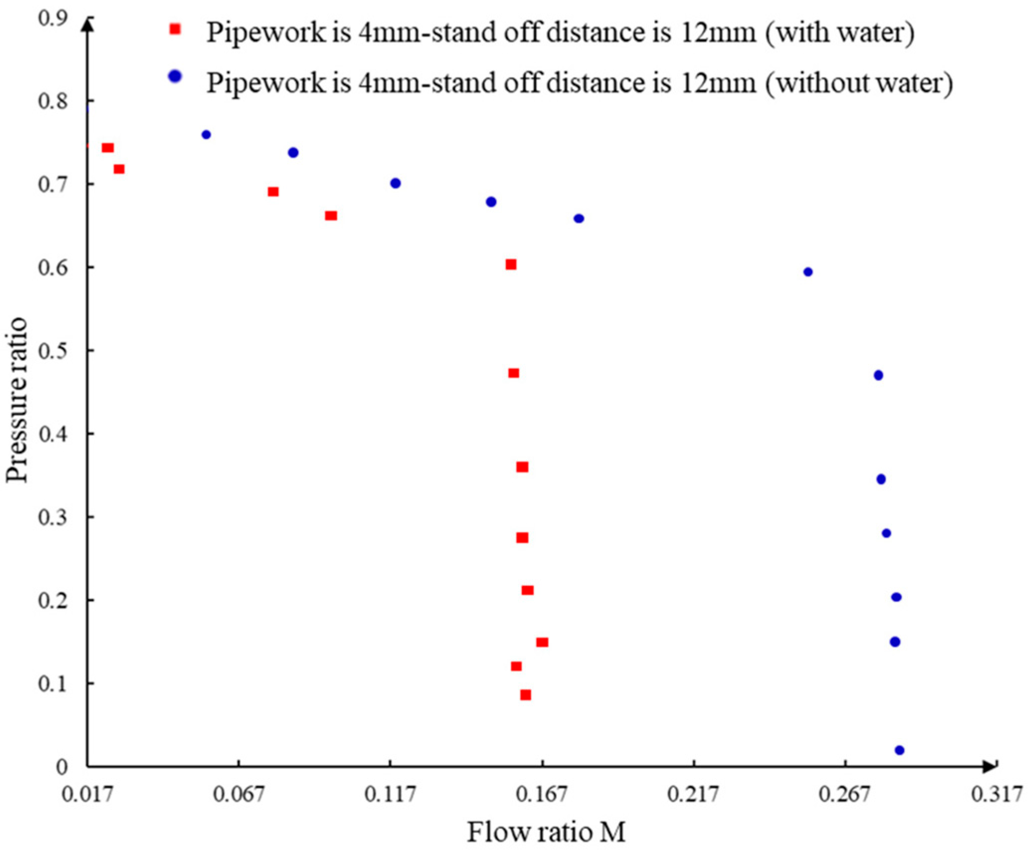
3.3.3. The Impact of Hydraulic Pressure on the Operational Performance of a Jet Pump

In Figure 14, Figure 15 and Figure 16, the experimental simulation of the jet pump’s negative-pressure sand suction was carried out only under the harsh operating conditions of no powered fluid and relatively low hydraulic pressures. Under actual operating conditions, the sand suction capacity and efficiency of the jet pump would be greatly improved. In this experiment, the jet pump achieved a suction capacity of up to 14 L/min and a maximum lift pressure $P_2$ of 9 MPa at a pump pressure of 30 MPa, with a pump efficiency of 18%. Under conditions of an equal pump pressure, throat diameter, and nozzle throat distance, increasing the hydraulic pressure resulted in a greater suction capacity of the jet pump, while the maximum lift pressure $P_2$ remained relatively constant. The efficiency of the jet pump also improved when operating with powered hydraulic pressure.

3.3.4. The Impact of Nozzle Area Ratio on the Operational Performance of a Jet Pump

In the initial theoretical analysis of the jet pump in this project, we discovered that the area ratio plays a crucial role in influencing both the efficiency and lifting performance of the jet pump. Different area ratios in jet pumps lead to varying lifting capacities and suction efficiencies. Figure 17, Figure 18 and Figure 19 illustrate that, during the experimental phase, we manipulated the area ratio of the jet pump by adjusting the nozzle throat distance. Specifically, our jet pump configuration included throat diameters of 3.5 mm and 4 mm, paired with a nozzle diameter of 2.5 mm, resulting in two area ratios: 0.3 and 0.4. By maintaining a nozzle throat distance of 12 mm and varying the pump pressures, we examined the impact of the area ratio on the jet pump’s efficiency.

The variation in the area ratio has a minor influence on the suction capacity, lift pressure ratio, and suction efficiency of a jet pump. This is observed when using a nozzle with a diameter of 2.2 mm and a nozzle throat distance of 12 mm, all under conditions of zero inlet pressure. Nonetheless, it does exert a substantial effect on the lift pressure ratio and suction efficiency of the jet pump. Increasing the area ratio to 0.3 within the jet pump leads to a higher lift pressure and enhanced efficiency.

4. Experimental Evaluation of Sand Jetting Capability of Negative-Pressure Sand Jetting Tool

Based on the aforementioned experiments, we verified the sand-carrying capacity of the tool assembly through wellbore simulation testing, as shown in Figure 20. This test assesses the effectiveness of sand bed suction.

Four sand-flushing tests were conducted using a simulated wellbore as the reference point for the sand surface height. The initial sand surface height was considered as the zero point, with an increasing height towards the bottom of the well. We recorded displacement, variations in the sand surface height, and duration for each group. This data allowed us to calculate the sand-flushing velocity using the negative-pressure sand-flushing tool, as detailed in

Table 4. Experimental data recording form for negative-pressure sand jetting.

Number	Displacement (L/min)	Initial Height of Sand Surface (cm)	Decreased Height of Sand Surface (cm)	Duration (s)	Flush Velocity (m3/d)
1	59.79	0	69	320	2.65
2	59.26	69	104	120	3.58
3	59	116	134	90	2.46
4	59	134	158	190	1.55

.

Experimental Results of Wellbore Simulation Test

Through the wellbore simulation experiments, we observed that, when the pump pressure was maintained at 25 MPa and the pump displacement at 60 L/min, the negative-pressure jetting tool efficiently suctioned the sand bed with a descent height of at least 52 cm within 10 min, all within a 5 1/inch wellbore. The experimental operating parameter curve is shown in Figure 21. To gain insight into the tool’s operational status, we did not raise the tool at a descent speed of 0.5 m/min. Consequently, we could not measure the tool’s maximum sand suction efficiency.

Based on this data analysis, we successfully validated the sand suction capability of the negative-pressure jetting tool under typical operating conditions. Additionally, the tool’s parameters can accommodate jetting pressure increases of 10 MPa or more. This makes the tool suitable for low-pressure loss wells with depths of 3000 m and horizontal sections of 800 m.

5. Conclusions

• This paper presents a design methodology aimed at achieving the optimal pump efficiency while ensuring the minimum required lifting pressure ratio. It calculates the optimal structural parameters for a jet pump. The characteristic and efficiency equations of the jet pump, derived from the principle of energy conservation, illustrate the interrelationships among the area ratio, pressure ratio, flow rate ratio, and density. It is our contention that optimizing pump efficiency is the ideal approach for jet pump design. However, the parameter optimization method based on the P-M curve has inherent limitations, necessitating the development of an engineering design evaluation method focused on maximizing suction force.
• The jet pump can achieve the suction of solids under relatively low pump pressure conditions. With an increasing pump pressure, the suction capacity of the jet pump remains relatively constant, while the lifting capacity increases.
• The jet pump can effectively suction solids at relatively low pump pressure conditions. As the pump pressure increases, the suction capacity of the jet pump remains stable, while its lifting capacity improves.
• The presence of dynamic fluid within the formation significantly impacts the sand suction capability of the jet pump. When exposed to dynamic fluid pressure, the jet pump’s suction capacity increases significantly, while its lifting capacity remains relatively constant.
• Through a blend of experimental and theoretical methods, we gained valuable insights into how process parameters, sand-flushing capabilities, and the overall efficiency of jet pumps interact. Nonetheless, it is crucial to recognize the limitations of our approach. While the combination of experiments and theory offered comprehensive insights, our study mainly concentrated on a specific range of parameter variations. A more comprehensive understanding of jet pump behavior and the revelation of nuanced relationships could be achieved by exploring a wider spectrum of parameter combinations.

References

1. Dong, P.; Lang, Z.; Xu, X. The Fully Coupled Fluid-solid Analysis for the Reservoir Rock Deformations Due to Oil Withdrawal. J. Geomech. 2000, 6, 5. [Google Scholar]
2. Gao, G.W.; Li, L.P.; Song, X.J. A new technique for the real-time monitoring of the sand producing in heavy oil wells. J. Xi’an Shiyou Univ. Nat. Sci. Ed. 2010. Available online: https://www.researchgate.net/publication/290279923_A_new_technique_for_the_realtime_monitoring_of_the_sand_producing_in_heavy_oil_wells (accessed on 27 July 2023).
3. Mu, J.F.; Lv, Y.X.; Wei, S.L.; Jiang, Y.Q.; Liu, Y.M. Research and Application on the Technology of Relieving Reservoir Plugging from Ultra-Deep Oil Well. Oilfield Chem. 2010, 27, 149–152. [Google Scholar] [CrossRef]
4. Wu, J.; Yuan, D.-Q.; Wang, G.-J. Current situation and prospect of jet pumps. J. Drain. Irrig. Mach. Eng. 2007, 25, 65–68. Available online: https://en.cnki.com.cn/Article_en/CJFDTOTAL-PGJX200702017.htm (accessed on 27 July 2023).
5. Walker, C.I.; Bodkin, G.C. Empirical wear relationships for centrifugal slurry pumps-Part1: Side-liners. Wear 2000, 242, 140–146. [Google Scholar] [CrossRef]
6. Leontiev, D.S.; Kleshchenko, I.I.; Tsedrik, N.S. Technology of Reduction of Sand Production in Oil Wells. Oil Gas Stud. 2017, 5, 72–74. [Google Scholar] [CrossRef]
7. Wen, Y.; Li, H.; Zhu, Y.; Song, Z.; Wang, Y.; Jin, J. Sand Control Technology for Low pressure Lost-Circulation Wells and Application in South Sudan. J. Phys. Conf. Ser. 2022, 2152, 012013. [Google Scholar] [CrossRef]
8. Qu, Z.Q.; Su, C.; Wen, Q.Z.; Chang, K. Optimal Design of Parameters of Sand Control by Frac-packing. Spec. Oil Gas Reserv. 2012, 19, 134–137+148. Available online: https://www.semanticscholar.org/paper/Optimal-Design-of-Parameters-of-Sand-Control-by-Kun/162a1969a79ba70a8a131ec9a0808ec482e0efab#citing-papers (accessed on 27 July 2023).
9. Rafferty, P.; Ennis, J.; Skufca, J.; Craig, S. Enhanced Solids Removal Techniques from Ultra Low Pressure Wells Using Concentric Coiled Tubing Vacuum Technology. In Proceedings of the SPE/ICoTA Coiled Tubing and Well Intervention Conference and Exhibition, The Woodlands, TX, USA, 20–21 March 2007. [Google Scholar] [CrossRef]
10. Wang, C.B.; Lin, J.Z.; Shi, X. Numerical Simulation and Experiment on the Turbulent Flow in the Jet Pump. J. Chem. Eng. Chin. Univ. 2006, 20, 175–179. [Google Scholar]
11. Wen, J.; Yu, B.; Lu, H.; Cui, T.; Zhu, Z. Large eddy simulation for jet pump flow. Eng. J. Wuhan Univ. 2007, 2, 110–114. [Google Scholar]
12. Zhao, Y.; Chen, Y.; Wang, X.; Wang, B.; Xu, Y. Numerical simulation on influence of central nozzle-to-throat clearance on performance of compound jet pump. Water Resour. Hydropower Eng. 2019, 50, 120–126. [Google Scholar] [CrossRef]
13. Berlemont, A.; Desjonqueres, P.; Gouesbet, G. Particle lagrangian simulation in turbulent flows. Int. J. Multiph. Flow 1990, 16, 19–34. [Google Scholar] [CrossRef]
14. Powell, C.J. Differences in the Characteristic Electron Energy-Loss Spectra of Solid and Liquid Bismuth. Phys. Rev. Lett. 1965, 15, 85854. [Google Scholar] [CrossRef]
15. Liu, B.; Hui, X.; Yang, T.; Yin, L.; Guo, W. Experimental Study on Fatigue Behavior of Concentric Coiled Tubing. China Pet. Mach. 2018, 46, 110–115. [Google Scholar] [CrossRef]
16. Citrini, D. Study of the Theory of the Jet Pump. Energ. Elettriea 1948, 25, 12. [Google Scholar]
17. Fried, S.J.; Bell, P.G.; Sask, D.E.; Ranks, R.D. The selective evaluation and stimulation of horizontal wells using concentric coiled tubing. In Proceedings of the International Conference on Horizontal Well Technology, Calgary, AB, Canada, 18–20 November 1996. [Google Scholar] [CrossRef]
18. Falk, K.; Fraser, B. Concentric Coiled Tubing Application for Sand Cleanouts in Horizontal Wells. J. Can. Pet. Technol. 1998, 37, 46–50. [Google Scholar] [CrossRef] [PubMed]
19. Gosline, J.E.; Orrien, M.P. The Water Jet Pump. Univ. Calif. Pub. Eng. 1934, 3, 160–200. [Google Scholar]
20. Ge, Y.-J.; Ge, Q.; Yang, J. Numerical Simulation and Confirming of Optimal Range on the Nozzle-to-throat Clearance of Liquid-gas Jet Pump. Fluid Mach. 2012, 40, 21–24. Available online: https://kns.cnki.net/kcms2/article/abstract?v=3uoqIhG8C44YLTlOAiTRKgchrJ08w1e7fm4X_1ttJAkWyZi1rsL0-2YN2C7vUCGdFEJ4Fx4egm-zK89lP1oXHX6WJ76J2njY&uniplatform=NZKPT (accessed on 27 July 2023).
21. Zhu, J. Application of horizontal wells open hole gravel pack sand-control completion technology. Oil Drill. Prod. Technol. 2010, 32, 106–108+112. [Google Scholar] [CrossRef]
22. Lu, H. Injection Technique Theory and Application; Wuhan University Press: Wuhan, China, 2004; pp. 1–53. [Google Scholar]
23. Wang, C. The Well Drainage Sand with Jet Pump Research. Ph.D. Thesis, Zhejiang University, Zhejiang, China, 2004. [Google Scholar]
24. Lv, Z.; Wang, Y.; Liu, J.; Cao, P. Value of Nozzle Falloff Angle of Jet Pump. J. Jiangsu Univ. Nat. Sci. Ed. 2015, 36, 7. [Google Scholar]
25. Tan, J.; Zhu, J.M.; Long, X.P. Numerical analysis of nozzle Length-diameter ratio of liquid jet pump. J. Hydropower Energy 2019, 37, 151–154. [Google Scholar]
Figure 1. Basic structure diagram of jet pump.
Processes 11 02841 g001
Figure 2. Parameter optimization design method.
Processes 11 02841 g002
Figure 3. Pump efficiency curve under ideal conditions.
Processes 11 02841 g003
Figure 4. PM curve at pump pressure of 50 MPa and pump displacement of 70 L/min.
Processes 11 02841 g004
Figure 5. PM efficiency curve at pump pressure of 50 MPa and pump displacement of 70 L/min.
Processes 11 02841 g005
Figure 6. Experimental setup for wellbore simulation test.
Processes 11 02841 g006
Figure 7. Pump pressure versus suction flow curve.
Processes 11 02841 g007
Figure 8. Suction capacity curve of throat with a nozzle diameter of 3.5 mm and a spray distance of 6 mm.
Processes 11 02841 g008
Figure 9. PM curve for throat with a nozzle diameter of 3.5 mm and a spray distance of 6 mm.
Processes 11 02841 g009
Figure 10. The efficiency curve of throat with a nozzle diameter of 3.5 mm and a spray distance of 6 mm.
Processes 11 02841 g010
Figure 11. The suction volume curves at various nozzle throat distances under a pump pressure of 30 MPa.
Processes 11 02841 g011
Figure 12. PM curves for different throat spacings at pump pressure of 30 MPa.
Processes 11 02841 g012
Figure 13. Efficiency curves at various throat clearances under a pump pressure of 30 MPa.
Processes 11 02841 g013
Figure 14. The curves of suction volume at various hydraulic power pressures under a pump pressure of 30 MPa.
Processes 11 02841 g014
Figure 15. The PM curves of hydraulic power at various dynamic hydraulic pressures, with a pump pressure of 30 MPa.
Processes 11 02841 g015
Figure 16. The efficiency curves of various hydraulic power units at a pump pressure of 30 MPa.
Processes 11 02841 g016
Figure 17. The suction volume curves for different area ratios at a pump pressure of 30 MPa.
Processes 11 02841 g017
Figure 18. The PM curves for different area ratios at a pump pressure of 30 MPa.
Processes 11 02841 g018
Figure 19. The efficiency curves for various area ratios under a pump pressure of 30 MPa.
Processes 11 02841 g019
Figure 20. The simulated sand height within the wellbore and the sand particles extracted, suctioned, and collected.
Processes 11 02841 g020
Figure 21. Pump displacement performance curve.
Processes 11 02841 g021