A simulation model based on AMESim is used to experimentally test the proposed intelligent algorithm due to the dearth of data in real production. The suggested approach is implemented on MATALB R2022b using a computer with the device configuration of an Intel Core i7-13700K processor, an NVIDIA GeForce RTX 3070 graphics processor, and 32 GB of RAM.
4.1. Pressure Injection System Modeling
The simulation model of the pressure injection mechanism is constructed using AMESim and is depicted in
Figure 7 in accordance with the operation of the hydraulic system of the pressure injection mechanism and the real component parameters.
The specific action process is as follows:
Slow phase: The solenoids of valves 420 and 414a are both turned on at the same time. Oil from the pressure injection accumulator enters the rodless chamber of the pressure injection cylinder through valve 420, flows out of the rodded chamber through valve 414a, and the cylinder slowly moves forward. The speed of the slow phase is controlled by valves v414a and v420. In this experimental model, the duration of this phase is 3 s, and the preset velocity is 0.5 m/s.
Fast phase: When the displacement sensor on the pressure injection cylinder determines that the cylinder has reached the position of rapid pressure injection, the solenoids of valves v414 and v419 are simultaneously turned on. At this time, oil from the pressure injection accumulator primarily enters the rodless cavity of the cylinder through valve v419 and exits the rodded cavity of the cylinder through valve v414. The speed of the fast phase is controlled by valves v419 and valve v414. In this experimental model, the duration of this phase is 0.14 s, and the preset velocity is 4 m/s.
Pressurization phase: The solenoid of valve v428 is activated as the punch quickly pushes the liquid metal to fill the cavity. Through valve v428, the oil in the pressurizing accumulator flows into the right chamber of the pressurizing cylinder, causing the piston of the pressurizing cylinder to move to the left, and valve v428 completes the control of the pressurizing phase. In this experimental model, the duration of this phase is 1.86 s, and the pressurized accumulator is preset at 160 bar.
This study chooses the five performance indicator groups of fast speed accuracy, slow speed accuracy, acceleration performance, braking performance, and pressure accuracy for evaluation in accordance with the real production needs. The performance index is defined as
q due to the various production constraints. For instance, the acceleration performance index
qa is defined as follows:
where
ac is the desired target acceleration,
ai is the measured actual acceleration, and
k is a scaling factor to meet different production requirements. The maximum value of
q is 100, which represents the ideal situation in which the actual performance and the desired performance are exactly the same. The lower the value of
q, the poorer the real performance turns out to be.
The performance deterioration of valves v414, v414a, v419, v420, and v428 is the element impacting the performance index, according to workflow and maintenance experience in actual production; therefore, these five components are selected as the aim of component classification.
4.2. Creation of the Sample Set
The following eight sets of signal data for the chosen stages are derived by AMESim simulation based on the signals that can be recorded in the actual pressure injection mechanism, as illustrated in
Figure 8.
The displacement signal of the pressure injection cylinder, the pressure signal of the rodless chamber and the rodded chamber, and the current signals from the valves v414, v414a, v420, v419, and v428 are the signals used, respectively. The above three processes take a total of 5 s, and the signal is sampled at a frequency of 1000 Hz with a time interval of 1 ms.
The speed of the simulation model is adjusted to 4 m/s in the rapid phase and 0.5 m/s in the slow phase, and
Figure 9 depicts the velocity curve of the pressure injection cylinder.
In this paper, the total number of samples obtained through simulation is 480 (80 × 6) based on the division of low-performance component types, of which the number of samples in the training set is 384 (64 × 6) and the number of samples in the test set is 96 (16 × 6).
Based on the factory production requirements, the threshold value for component classification is calculated by Equation (11) as shown in
Table 2, and if the performance index is lower than this value, it is recognized as the presence of low-performance components.
4.3. Training of the Model and Analysis of Results
The fewer samples used, taking into consideration computation costs and calculation times, the better due to actual production needs. Therefore, the selection of sample size is made by using various sample sizes for testing and training. The average accuracy for classifying low-performance components after ten 5-fold cross-validation passes is shown in
Table 3.
The
R2 coefficient of determination is used to examine the effect of performance evaluation. It measures how well the anticipated value matches the observed value and is determined as follows:
where
n is the number of samples,
is the performance evaluation index of the
ith sample,
ri is the actual performance index of the
ith sample, and
is the average performance index of the actual sample. The closer the value of
R2 is to 1, the closer the predicted value is to the actual value. The average
R2 values of the performance metrics determined after 10 5-fold cross-validations are presented in
Table 4.
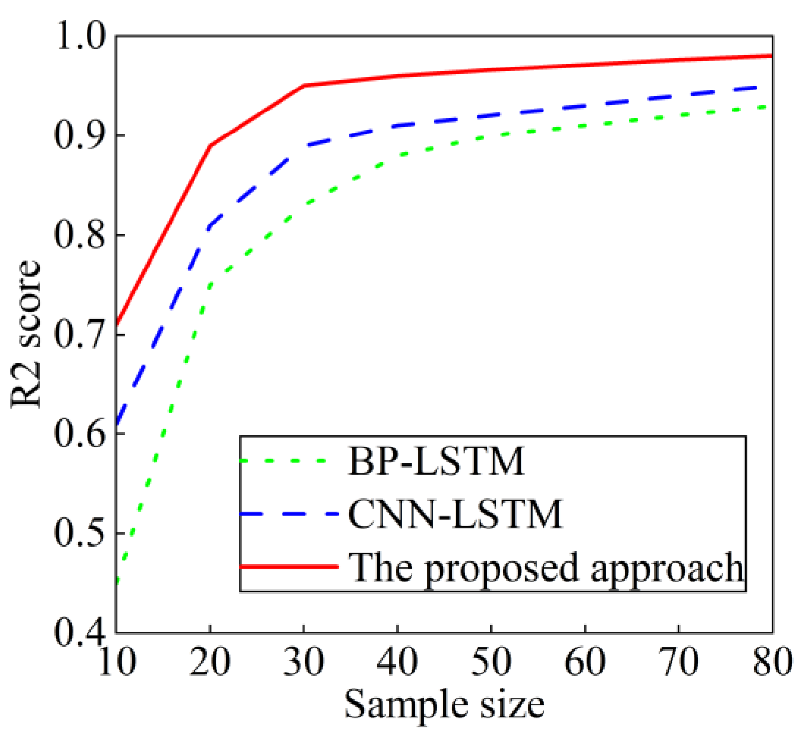
The line graphs associated with the above two tables are shown in
Figure 10 and
Figure 11.
From the above tables and figures, it can be seen that as the number of samples increases, the classification and performance evaluation of all the intelligent algorithms are getting better. The method proposed in this paper has a much higher accuracy and R2 value than the other two single methods when the sample size is small. Furthermore, as the number of samples increases, it can quickly reach a high accuracy and R2 value. Compared with stacking ensemble methods, DS methods have higher accuracy when the sample size is small. However, as the sample size increases, the accuracy of stacking will be higher than that of the DS method. This has been analyzed as a result of the poor performance of the base model with a small sample size and the small number of base models used in this paper.
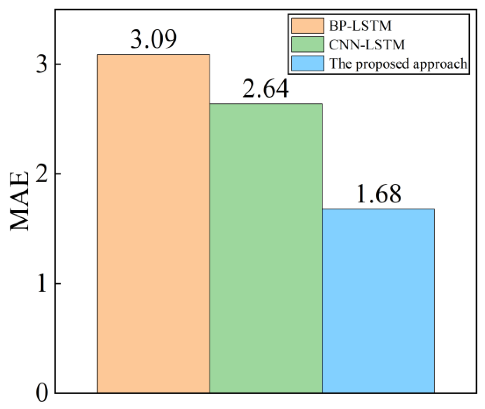
The proposed method achieved a classification accuracy of 95.67% under a sample size of 40 × 6, which is comparable to that of CNN-LSTM with a sample size of 80 × 6, which achieved 95.87% accuracy. Similarly, the
R2 value of the proposed method under the sample size of 40 × 6 is 0.947, which is also comparable to that of CNN-LSTM under the sample size of 80 × 6, which achieved a value of 0.951. The average MAE values for performance evaluation at the 40 × 6 sample size are shown in
Figure 12.
As seen above, the method proposed in this paper has produced excellent results in component classification and performance evaluation when the number of samples is more than 40 × 6. The performance of BP-LSTM and CNN-LSTM improves significantly as the number of samples rises, and while the proposed method still performs better than the other two methods, the performance gap between them is gradually closing. This paper employs a sample set of 40 × 6 for additional testing, taking into account the practical use and computing cost.
In order to test the stability of the proposed model, a one-time 5-fold cross-validation of the three methods mentioned above is performed. The accuracy and R2 values obtained for each of the low-performance component classifications and performance evaluations are shown in
Table 5 and
Table 6, and the corresponding line graphs are shown in
Figure 13 and
Figure 14.
The two figures above show that the performance of the two approaches without information fusion fluctuates, and the suggested method beats the other two ways in terms of stability in addition to having a better accuracy and R2 value.
The confusion matrix demonstrates that a single intelligent algorithm has significant accuracy swings when categorizing a particular class of components, although it has a respectable average accuracy. The following tags provide examples: Tag 2 (Valve v420), Tag 5 (Valve v428), and Tag 6 (Normal Performance). The method proposed in this study effectively resolves the issue of conflicting information sources through the information fusion of algorithm results, not only in the classification of tags 2 and 6 with 100% accuracy but also in tag 5 with increased accuracy. In addition, it can be seen that the single algorithm is not considered ideal for the classification of tag 5, and the stack algorithm does not get a good performance boost for the classification of tag 5 because it is affected by the performance of the base model. As a result, the method not only has high accuracy but also good stability in categorizing a specific class of components.
As regards the degree of fitting for the performance metrics of specific samples, take the acceleration performance metrics as an example. Regarding the degree of fit for a particular sample of performance metrics, the result of comparing the performance evaluation metrics with the actual performance metrics, using acceleration performance metrics as an example, is shown in
Figure 19.
The graph shows that the method suggested in this study on some samples, where the single intelligent algorithm cannot achieve good evaluation results, through the neural network to the outcomes of the information fusion and therefore get comparatively good evaluation results.


