Abstract
New biofuels are in demand and necessary to address the climate problems caused by the gases generated by fossil fuels. Biohydrogen, which is a clean biofuel with great potential in terms of energy capacity, is currently impacting our world. However, to produce biohydrogen, it is necessary to implement novel processes, such as Pressure Swing Adsorption (PSA), which raise the purity of biohydrogen to 99.99% and obtain a recovery above 50% using lower energy efficiency. This paper presents a PSA plant to produce biohydrogen and obtain a biofuel meeting international criteria. It focuses on implementing controllers on the PSA plant to maintain the desired purity stable and attenuate disturbances that affect the productivity, recovery, and energy efficiency generated by the biohydrogen-producing PSA plant. Several rigorous tests were carried out to observe the purity behavior in the face of changes in trajectories and combined perturbations by considering a discrete observer-based LQR controller compared with a discrete PID control system. The PSA process controller is designed from a simplified model, evaluating its performance on the real nonlinear plant considering perturbations using specialized software. The results are compared with a conventional PID controller, giving rise to a significant contribution related to a biohydrogen purity stable (above 0.99 in molar fraction) in the presence of disturbances and achieving a recovery of 55% to 60% using an energy efficiency of 0.99% to 7.25%.
1. Introduction
Currently, oil sources, which are the largest energy generators, are running out; their excessive misuse has created an environmental impact on our ecosystem. Consequently, there is global warming due to the increase in polluting gases from using these fossil fuels. As a result, to reduce this impact, some biofuels can be utilized that do not have a more significant effect on the environment than fossil fuels, such as biohydrogen. Various companies are investing in obtaining these biofuels or managing to produce energy by accelerating energy transition. However, to achieve 99% purity, various technological processes must be implemented to separate this compound from others. One of these processes to obtain a high degree of purity is the Pressure Swing Adsorption (PSA) process [,,,,,,]. This PSA process is a method of separating gas mixtures using adsorbents (natural or synthetic zeolites). Different types of research related to the PSA process has been conducted, and some developments have adapted different start-up conditions with multiple operating conditions. Some of these conditions are to have higher recovery with a high degree of purity [,,,,,]. However, these processes operate in cyclical conditions to produce a constant product (purity) that generates complexity in the PSA process, since various variables such as pressure, temperature, flow, flow rate, and composition are involved, as well as the characterization of the value proportional valves for opening and closing at each stage of the process. The highly nonlinear model of this process is represented by Partial Differential Equations (PDEs) [,,]. Contemplating the aforementioned, it is very likely that the purity will decline and 99% of the biohydrogen obtained will be lost, since there may be disturbances (unwanted inputs) that can have an effect on the product obtained. Therefore, it is necessary to implement controllers in this type of complex process that can benefit and keep the purity of biohydrogen stable at 99%, managing to attenuate these disturbances. In this work, the purities of H2 obtained were 99.995%, 99.9141%, and 99.998%, using an energy efficiency of 1.9%, 1.5%, and 2.4%. The recoveries achieved were 73%, 79%, and 70%; however, these data may decline because they are uncontrolled processes.
Little research and development has impacted the control of the PSA process for the production of biohydrogen; however, the extant work is of great importance to justify and present the innovation of this scientific work with a significant contribution. One of these works is the one presented by [], in which they design a Robust stabilizing Infinite-Horizon Model Predictive Controller (RIHMPC) applied to the PSA process to separate the H2/CO2 mixture. To achieve the design of this controller, they chose to identify various linear models at each point of operation of the PSA process; as a result, they were able to keep a PSA plant stable at different points of operation. With this controller, a CO2 recovery of 97% was obtained with a purity of 0.87% during 200 operating cycles.
In [], a Deep-Learning-oriented Economic Model Predictive Control (EMPC) strategy was used to separate and test the H2/CO2 mixture. For the controller design, reduced models based on a structure based on a Deep Learning Neural Network (DNN) were used. The EMPC achieved a reduction in computational expense for its hydrogen purity predictions and also generated a high CO2 recovery and productivity under scenarios with the presence of disturbances. The CO2 recovery achieved has a variation generated by the disturbance between values from 99% to 85% to be obtained with a CO2 purity of 86.5 to 84 in molar fraction. Based on these unwanted inputs, the hydrogen productivity obtained ranged between 3.3 and 3.2 in molar fraction with no validation with a rigorous PSA model, despite the promising results. Subsequently, different works were developed that use controllers applied to the same PSA process to purify and separate different mixtures: medical-grade oxygen, bioethanol, and biomethane. These works consider controllers such as Active Fault-Tolerant Control, State Feedback Control, and Model Predictive Control. The design procedure of these controllers uses reduced models from the input and output data of the PSA process. The results are outstanding since they keep the process stable and attenuate disturbances at the process’s input, reducing the effect of faults in the feed valve [,,,].
We have found different works in the literature related to PSA control, in particular, we have observed that most of the designed controllers are compared with PID, and this is because PID control is widely used in industry (experimental processes) [,,,,,,]. Let us point out that, due to the complexity of this PSA process, it is necessary to make comparisons with different control strategies aiming at observing how robust they can be in different scenarios. With this in mind, based on the fact that LQR controllers (within the optimal control theory) can find an optimal control gain such that the control objectives are accomplished, it is worth exploring them for the PSA process addressed in this paper. Notice that, finally, the importance of LQR controllers in the experimental context refers to the fact that the closed-loop system behavior will be optimal due to a cost function minimizing procedure regarding optimal control theory.
The contribution of this work is focused on producing biohydrogen at 99.99% for use as biofuel by applying optimal control theory, aiming at performing a comparison with the control strategies previously considered. Implementing these controllers will allow attenuating disturbances at the input of the PSA process and keep the biohydrogen feat stable. The PSA plant has a highly nonlinear process behavior that involves several variables with a pseudosteady state, which is a complicated challenge. However, the development of the stages of this work gives a pertinent solution of how it is possible to approach the subject. It generates a unique biohydrogen production solution and achieves a robust PSA plant against unwanted inputs.
This article is sectioned as follows: Section 2 shows the rigorous PSA model and the appropriate characteristics with nominal values to produce 95% biohydrogen. Section 3 presents the identified model developed from the inputs and outputs generated by the rigorous PSA model and a detailed description of the discrete LQR controller design developed from the identified model. In Section 4, the discrete LQR controller is implemented on the identified model, and results are obtained before trajectory changes in biohydrogen purity. Section 5 presents the validation of the discrete LQR controller on the PSA plant that produces biohydrogen. Section 6 shows the conclusions that make a significant contribution to the production of biohydrogen.
2. Separation and Production of Hydrogen by PSA
The PSA plant is a process with two columns packed with type 5A zeolite connected in parallel; to get the gas to pass from one column to another, 10 proportional valves are implemented. The start-up parameters (nominal values) are presented in Figure 1.
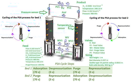
Figure 1.
Schematic diagram of the PSA plant (production of biohydrogen).
The PSA processes comprise a feed of synthesized gas (H2: 0.69, CH4: 0.03, CO: 0.02, CO2: 0.26). This gas passes through bed 1 to carry out the adsorption step for 70 s to begin to produce hydrogen; at the same time, the purge step is carried out in bed 2 using a pressure of 100 kPa to release all the active sites of the type 5A zeolite that are inside the columns. Subsequently, the depressurization and repressurization steps are presented for 3 s. The depressurization is carried out in bed 1, and with this step, part of the compounds adsorbed on the type 5A zeolite are released. The repressurization is carried out in bed 2 to elevate a pressure of 100 kPa to 980 kPa; with this elevated pressure, bed 2 is ready for the adsorption and hydrogen production step. The next steps are the purge for bed 1 and the adsorption for bed 2. Bed 2 reaches a high pressure and begins to absorb and retain the compound to purify hydrogen for a time of 70 s. On the other hand, bed 2 begins the purge step to completely release the active sites of the type 5A zeolite and become free to adsorb compounds again. This purge step must bring the pressure from 150 kPa to 100 kPa. Finally, the repressurization and depressurization steps are performed for beds 1 and 2 for 3 s. Repressurization is carried out in bed 1 and elevates the pressure from 100 kPa to 980 kPa to leave bed 1 in appropriate conditions to adsorb compounds and produce hydrogen. For bed 2, meanwhile, the depressurization step decreases the pressure from 980 kPa to 150 kPa.
This series of steps is repeated until an operation cycle is completed. As a result, high hydrogen production is purified at each cycle until the CSS is reached and a purity of 0.9485 in molar fraction is obtained.
It is necessary to implement proportional valves to let the gas pass at established times to ensure that the sequence of steps works appropriately, as shown in Figure 1.
Type 5A zeolite can withstand high temperatures and pressure changes with less deterioration than other adsorbents. The adsorption capacity for each gram of adsorbent is CH4: 0.030, CO2: 0.202, CO: 0.049, and N2: 0.238, achieving hydrogen with a high purity.
The PSA model used was obtained from the work in [,,]. This PSA plant presents PDEs of the mass balance (gas phase), energy balance (gas phase), pressure drop, and kinetic models for solid and Langmuir equations, with the following considerations:
- The gas in the beds conforms to the ideal gas equation.
- The radial axis of pressure, concentration, and temperature is not assumed.
- The axial pressure drop is negligible.
- The LDF model is used to generate the mass transfer rate.
- Extended Langmuir is used to determine the adsorption and desorption of the gas.
Table 1 shows the set of PDE equations. In order to solve these equations, it is necessary to consider initial and boundary conditions (see Table 2).

Table 1.
Equations used for the PSA plant.
Table 2.
Use of initial and boundary conditions.
The PSA performance was measured by calculating the productivity and recovery of the biohydrogen by the following Equations (1) and (2):
Biohydrogen Production from Startup to CSS Using the PSA Process
The start-up of the PSA plant is from a composition of synthesized gases (H2: 0.69, CH4: 0.03, CO: 0.02, CO2: 0.26). The profiles of the compounds can be observed in Figure 2, as well as how they increase or decline in purity. In the hydrogen profile, it is observed that after four operating cycles, the hydrogen purity increases with each cycle that passes, and the Cyclical Stable State (CSS) is achieved with seventeen cycles, achieving a purity of 0.95 in molar fraction. On the other hand, compounds of methane, CO, and CO2 decrease to values of less than 0.2 in molar fraction. To achieve these results, a 980 kPa production pressure was considered, using a constant temperature of 298.15 K; likewise, the purge pressure to release the active sites of the type 5a zeolite was 100 kPa (see Figure 1 and Figure 2).
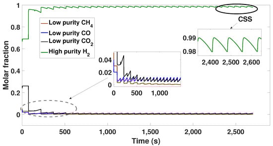
Figure 2.
Composition of the compounds from start-up to CSS (obtaining 95% hydrogen).
From the results shown in Figure 2, the identification of a reduced model capable of capturing the important dynamics of the PSA plant to produce biohydrogen was made. In order to identify a system, data were taken from the CSS. Input and output variables were considered through a sensitivity analysis, for which temperature was taken as a manipulated variable and hydrogen purity as a controlled variable. To understand this identification process in detail, it is necessary to review the work reported by [,].
3. Nonlinear Model Identified
As mentioned above, the input and output data were used to obtain a model identified from the rigorous PSA model to produce biohydrogen. The data used are shown in the papers in [,]. The result obtained from this identification is a Hammerstein–Wiener (H-W) model, depicted in Figure 3 and Figure 4a.
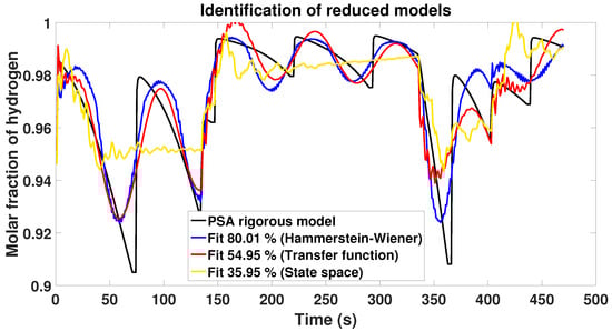
Figure 3.
Comparison of the different reduced models with approximation to the response generated by the PSA virtual plant.
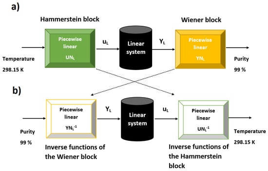
Figure 4.
(a) Identified H-W model; (b) H-W model with inverse functions.
Figure 3 shows the different reduced models used to approximate the response of the virtual PSA plant. A model was identified by a transfer function with 16 poles and 8 zeros, as well as a model represented in state space with 8 states; the fits obtained were 54.95% and 35.95%. From these results and aiming at improving the fit, the Hammerstein–Wiener representation was considered. This model can approximate the PSA dynamics better than the linear ones, since the Hammerstein–Wiener representation is nonlinear. The Hammerstein–Wiener identified model achieved a fit of 80.01%, as seen in Figure 3.
The H-W model is formed by two static nonlinear blocks at the input and output, as well as a linear dynamic model. The purpose of these nonlinear blocks is to capture the dynamics of the rigorous PSA model. Let us point out that the linear models cannot reproduce the PSA’s dynamics properly; for this reason, the H-W was selected. For the controller design, the linear dynamic model was used, along with the inverse functions of the Hammerstein and Wiener blocks, to couple the controller designed with the rigorous model (see Figure 4b). The static nonlinear function parameters and their inverses are observed in Table 3 and Table 4, and the linear dynamic model is presented in Equation (3).
with and .
Table 3.
Nonlinear input, piecewise linear.
Table 4.
Nonlinear output, piecewise linear.
From the parameters obtained in Table 3 and Table 4, the inverse functions of the Hammerstein and Wiener blocks are obtained. These are presented in Equations (4) and (5). Likewise, Equation (3) (Transfer Function) was converted to a space-state representation in discrete time, shown in Equation (6).
The discrete linear system is expressed as follows in discrete state-space representation:
where is a matrix associated to the vector states (), is a matrix associated to the input vector (), and is the matrix associated to the outputs () of the system. Within this representation, k is the sampling period considered (1 s).
After obtaining the inverse function equations of the Hammerstein and Wiener blocks, the design of the discrete LQR controller on the H-W model continues.
Discrete-Observer-Based LQR Controller Design
In order to design a control system able to ensure a desired biohydrogen purity for the system (6), a discrete-observer-based LQR controller characterized by the following diagram was considered:
The controller includes an integral action for the difference between the system output and an output desired value ; and a stabilizing term acting on the system state. From Figure 5, the control system is described by the following control law:
with and representing the stabilizing and integer control gains, respectively. In Equation (7) is the state estimation provided by a discrete Luenberger observer. Recall that the objective is to design an LQR observed-based controller with the aim of performing its comparison with what is commonly used in industries, a conventional PID controller. In addressing the control system design, let us point out that from control systems theory, it is possible to design the control and observer separately, from which the observer will be shown later, with the control law addressed as follows. Please keep in mind that for the control law, , was considered for design purposes. Firstly, notice the integer action characterized by
alternatively represented as
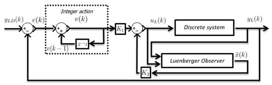
Figure 5.
Discrete-observer-based controller.
Now, by considering , Equation (7) is
with I as an identity matrix of compatible dimensions. For Equation (10), notice that Equation (6) and from Equation (7) were considered. Focusing on Equation (6) and Equation (10), with the consideration that is a linear combination of and , a new state-space representation can be obtained as
Following the control design, let us point out from Equation (11) that by considering , the vectors , and will be constant, ensuring , with no steady-state error as . As a consequence, by taking and , straightforward calculations result in
which can be represented as
with
and
As a result, the control gains will be computed by considering the following:
As such, notice the relevance of the system Equation (13), including an integral action aiming at ensuring a desired output value. Let us point out that with the objective of defining a suitable controller for a specific dynamical system, it is required to perform a comparison with different control strategies, from which the contribution of the present paper can be mentioned: the LQR controller performance in contrast with a conventional PID controller. Following the controller design from Equation (13), the Linear Quadratic Regulator (LQR) methodology is considered within this paper. The LQR method generally concerns optimal control theory, applied to dynamic systems involving an optimization problem. In this sense, an LQR controller aims at computing an optimal gain matrix K such that the state-feedback control minimizes the cost function:
subject to the state dynamics with Q, R, and N tuning parameters selected by the designer. This is, in turn, is considered for system (13) from the procedure shown throughout the present section, aiming at designing a control law for the study case shown in Equation (6). From LQR optimal control, it is expected to have a different dynamical closed-loop system evolution compared with the response obtained with a PID controller, hoping to conclude with a more suitable controller for the PSA process addressed throughout this paper. By using Matlab 2015b software with , , and , the following control gains were computed:
giving rise to from Equation (14) and concluding with the control design. As for the discrete Luenberger observer, in turn, notice that it will be in charge of providing the state estimation, giving rise to the need for its design. Recall that the Luenberger observer forms part of the control system due to (see Equation (7)), with the following general representation:
where L is the observer gain as a compatible dimensions vector with G, H, and C from Equation (6). Aiming at designing the observer, let us define the estimation error as with dynamics:
notice that L should be chosen in such a way that Equation (17) has eigenvalues within the unit simplex circle. As a result, L will ensure that as , which is the reason for the consideration in the controller design. For computing the observer gain, this paper’s results consider the pole placement allocation method within Matlab software, resulting in the following:
with absolute eigenvalues for Equation (17) as five elements equal to and the rest with a value of . These absolute values lie within the unit simplex circle, ensuring as . Finally, with control and observer gains computed, the control system is defined and ready for its application within the system (6).
4. Implementation of the Discrete LQR and Discrete PID Controllers on the H-W Model
After the design and tuning of the discrete LQR controller, the implementation in the H-W model continued; these tests were compared with the discrete PID controller.
Figure 6 represents the discrete LQR control scheme applied to the H-W model. It is observed that the output Wiener block and the inverse functions of the Wiener block are used.
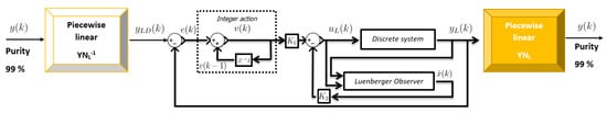
Figure 6.
Schematic of the discrete LQR controller on the H-W model.
Table 5 shows the cases presented before the implementation of the H-W model; these two cases present trajectory changes to verify the performance of each controller.
Table 5.
Reference changes on hydrogen purity (cases 1 and 2).
It can be seen in Figure 7a that for case 1, three reference changes are generated (see Table 5) with greater increases and decreases in biohydrogen purity. The purity varies depending on the established references. The discrete LQR controller presents a better approximation to the reference changes. However, in the reference change with a desired purity value of 0.702 in molar fraction, the purity has an undershot reaching a value near 0.6 in molar fraction for an instant of time of 20 s, and later, it is recovered to continue following the trajectory. In the case of the discrete PID controller, it is observed that the PID controller can follow the trajectory changes under the value of the international norms, but when the desired purity has a value of 0.999, the PID controller cannot follow the trajectory; in comparison, the LQR that has better performance. The discrete PID achieves approaching the set purity after a longer time compared with the shorter times generated by the discrete LQR controller (see Figure 7b).
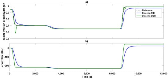
Figure 7.
(a) Hydrogen purity with three reference changes using the H-W model; (b) efforts of the discrete PID and discrete LQR controllers applied to the H-W model.
For case 2, six trajectory changes are generated (see Table 5) with small increases and decreases compared with case 1. In these tests, it can be observed how both controllers follow the established trajectory; however, the discrete PID controller continues presenting slower times responses and fails to quickly converge to the reference and cannot reach the purity desired value of 99%. On the other hand, the discrete LQR controller has no problem following purity changes and achieving 99% biohydrogen purity using adequate response times (see Figure 8a).
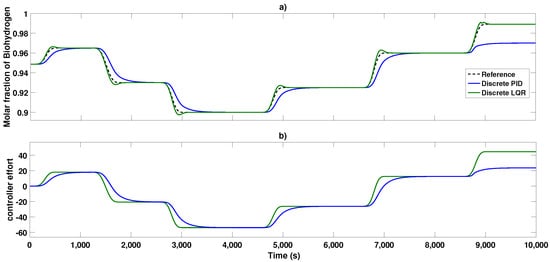
Figure 8.
(a) Hydrogen purity with six reference changes using the H-W model; (b) Efforts of the discrete PID and discrete LQR controllers applied to the H-W model.
Both controllers generate similar signals; however, the discrete LQR controller signal presents more effort with better response times compared with the discrete PID (see Figure 8b). From these results, we continue to validate the controllers in the PSA plant for the production of biohydrogen. In the following section, the implementation and validation are carried out on the rigorous PSA model defined by the equations shown in Table 1 and Table 2.
5. Validation of the Discrete LQR and Discrete PID Controllers Applied to the PSA Plant
This section is of great importance, since biohydrogen production, recovery, and purity are visualized in the presence of combined disturbances.
To achieve the implementation and validation of the LQR controller on the PSA biohydrogen plant, it is necessary to consider the nonlinear blocks of the Hammerstein and Wiener parts and the inverse of these functions. The control scheme implemented on the PSA plant is shown in Figure 9.
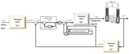
Figure 9.
Schematic of the discrete LQR controller on the PSA plant.
Two cases were presented for these tests, which are observed in Table 6. For case 3, the tests that were carried out determined how robust the controllers can be in the face of trajectory changes with the objective of increasing the biohydrogen purity from 95% to 99%. For case 4, the tests were more rigorous, since changes were implemented to obtain greater purity (above 99%) and maintain the purity stable in the face of three different disturbances that can affect the desired purity.
Table 6.
Reference changes in hydrogen purity (cases 3 and 4).
Figure 10 shows the results obtained from case 3. It can be seen that both controllers have different responses to trajectory changes in biohydrogen purity. However, the discrete PID does not follow the desired trajectory in the first change and is observed to have a slower response, which is reflected in not achieving the stated biohydrogen purity of 0.85 molar fraction. On the other hand, the discrete LQR controller presents control signals (temperature) with more significant effort to achieve its objective of following the established purity in short periods of time. The discrete LQR controller has better performance and robustness against these tests and can rapidly comply with the established trajectories and obtain a purity of 99%. Although the discrete PID in the first trajectory changes does not perform well, in the end, it is possible to obtain a purity of 99% biohydrogen.
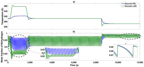
Figure 10.
(a) Temperatures generated by the discrete PID and discrete LQR controllers applied to the PSA plant; (b) hydrogen purity with three reference changes using the PSA plant.
Subsequently, to know the robustness of each controller, two trajectory changes with the presence of three disturbances are established in case 4. These perturbations were defined from the work carried out by [], where a sensitivity analysis is carried out and unwanted inputs can be defined that can affect the biohydrogen purity obtained. This scenario can be worrying for biofuel-producing industries, since not implementing controllers to keep the desired purity stable can negatively impact operating costs, since purity can drop and not meet the criteria or standards for use as biofuels.
The results for case 4 can be seen in Figure 11 and Table 7. The control signals generated by both controllers act based on the changes in trajectories and disturbances presented at the input of the biohydrogen-producing PSA process. For the discrete PID control, it is observed that the control signals require greater effort and present temperature values ranging from 295.15 K to 340 K (see Figure 11a); these are presented with the objective of rejecting or attenuating disturbances and achieving the desired purity of 99% biohydrogen. Therefore, when the discrete PID is implemented and the first disturbance (composition) can be observed that causes the purity of hydrogen to drop until it reaches values of 0.89 in molar fraction, the second disturbance that occurs is the supply pressure. This presents greater effect and causes the purity of biohydrogen to drop to 0.80 in molar fraction and, finally, the disturbance of the feed flow occurs, which causes the purity to drop from 0.999 to 0.901 in molar fraction. The three disturbances have a great effect on purity and manage to cause the desired purity to be lost for a few moments and does not meet international criteria or standards for use as biofuel. On the other hand, the discrete LQR controller has great performance and robustness in the face of these rigorous tests that decrease the purity when discrete PID control is implemented without a controller, as shown in Figure 11b. It can be seen that the control signals generated with the discrete LQR are smoother and have small temperature values (295.15 K to 299.15 K) that are used to mitigate or attenuate disturbances from the PSA process.
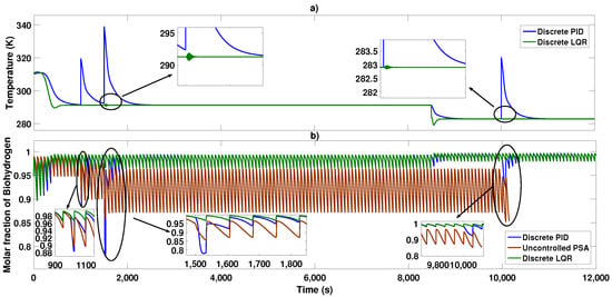
Figure 11.
(a) Temperatures generated by the discrete PID and discrete LQR controllers applied to the PSA plant; (b) hydrogen purity with two reference changes and perturbations combined using the PSA plant.
Table 7.
Case 4 with multiple disturbances.
We can also observe that without controllers, the purity of biohydrogen decreases, which indicates that it is urgently necessary to implement controllers in this highly nonlinear process (see Figure 11b). If there is no quick response from the operators or the process, this will generate an increase in energy, material, and economic costs to once again reach the desired purity of 99%.
Table 6 presents the facings obtained from the tests carried out with case 4. It is clearly observed that without a controller, it reaches a new pseudosteady state with a purity of 0.850 and 0.800 in molar fraction and does not meet the criteria for use as biofuel.
From the tests carried out (see Figure 11), it is possible to calculate and present the optimization of the biohydrogen production generated by the controllers, which implies obtaining a greater or lesser recovery or biohydrogen productivity using a minimum energy efficiency compared with the PSA process without automatic control. These indicators are necessary, since they contribute to knowing the performance that the PSA process can generate with the implementation of controllers when reaching the new CSS.
The cyclical reports provide valuable information to know the quantity and quality of the compound (biohydrogen). This can be known at each step and stage of the process, as well as the purity value in each of the valves that make up the PSA process; the results are from the beginning of the operation to the last cycle.
Results are calculated using the Recovery and Productivity Equations. These are shown in Equations (1) and (2).
Table 8 and Table 9 observe the optimal results of productivity and recovery. These tests were performed at 11 cycles (1500 s), where the disturbance (pressure) that generated the greatest effect on the biohydrogen purity was found (see Figure 11b).
Table 8.
Stream report (Biohydrogen productivity reached at 1500 s—Cycle 11).
Table 9.
Cycle recovery reports with control (Cycle 11).
From Table 8, it is observed that the composition material varies depending on the control actions that are generated at the feeding temperature. From these results, the total material is increased when the discrete LQR controller is used, generating higher purity (0.985 in molar fraction) as the final product at 11 cycles. However, it generates a higher enthalpy (17.25 MJ kmol−1) compared with the discrete PID and without a controller, which generates a purity of 0.830 and 0.800 in molar fraction using an enthalpy of 3.63 MJ kmol−1. In the case of the test without a controller, the results obtained are the opposite of the data obtained with the controllers. It can be seen that the purity achieved was 0.800 in molar fraction with an enthalpy of 44.5725 MJ kmol−1, which is greater than in all the cases presented. These are disturbing for a biohydrogen-producing PSA plant, which is why it is crucial and of significant contribution to implement controllers for this highly nonlinear process.
Likewise, the purity compositions of each compound when it passes through the main feed, waste, purge, and product valves can be seen in Table 8.
Subsequently, Table 9 shows the recovery obtained by the controllers and without the controller. The results were obtained from cycle 11, when the pressure disturbance occurred. In the results shown in Table 9, it can be observed that a greater recovery (60.116%) of biohydrogen is obtained when using the discrete PID controller compared with the discrete LQR controller, which obtains 53.8312%. However, the energy efficiency used for the discrete PID is higher (7.25%) compared with that used with the discrete LQR, which is 1.22%. Without a controller, biohydrogen recovery is higher (61.1303%); however, this product has a purity of 0.8000 in molar fraction, which is not suitable for use as biofuel. In addition, energy efficiency rises too high (20.8527%) compared with that obtained with controllers.
Table 10 and Table 11 show the optimal results of productivity and recovery. These tests were made at 69 cycles (10,000 s), where the disturbance (flow) is found, which is present when a purity of 99% biohydrogen is obtained (see Figure 11b).
Table 10.
Stream report (Biohydrogen productivity reached at 10,000 s—Cycle 69).
Table 11.
Cycle recovery reports with control (Cycle 69).
In Table 10, we can observe the total material of each compound and the composition that passes through the operating valves. From this rigorous test, in which a disturbance occurs at a purity point of 99.9% biohydrogen, it is possible to obtain optimal parameters of each controller. We observe that the purity obtained with the discrete PID controller is lower (0.901 in molar fraction), with 0.0025750 kmol of the final product and an enthalpy of 6.62234 MJ kmol−1. On the other hand, the discrete LQR controller generated a better purity of 0.999 in molar fraction with a lower enthalpy of 2.90687 MJ kmol−1. Without control, we can observe that the purity drops to 0.850 in molar fraction and that greater enthalpy (29.744 MJ kmol−1) is generated. Due to this, it is necessary to implement controllers to improve energy efficiency and maintain a stable purity of 99.99% biohydrogen.
Subsequently, Table 11 presents the recovery results using the discrete PID and discrete LQR controllers, as well as the results without a controller. We can see that the discrete PID controller has higher recovery compared with the discrete LQR controller; however, the energy efficiency used is higher (2.054%) compared with that generated by the LQR controller, which is 0.9968%. On the other hand, the results obtained without a controller show that a higher recovery (52.5512%) can be obtained, but with a purity lower than 0.850 in molar fraction using an energy efficiency of 9.29%. These uncontrolled results can cause great economic and material loss for the biohydrogen-producing industry.
6. Conclusions
For the first case, after three trajectory changes, the discrete LQR controller performs better than the discrete PID, since it follows the trajectory with better response times and achieves a biohydrogen purity of 99% in the last reference fit, in which case the discrete PID controller failed.
For the second case, using the H-W model, the controllers follow the purity defined as a reference. However, the discrete PID controller still has problems reaching the purity in the established time, and in the last trajectory change, it fails to reach the desired 99% pure biohydrogen. On the other hand, the LQR performs better and meets the objective of following the desired purity in the six reference sizes.
For the third case, the controllers were implemented in the PSA plant, where a highly nonlinear PDE model defines the process. The results are relevant and make a significant contribution, since it can be seen how the discrete LQR controller has good performance and can withstand the oscillatory complexity that the PSA plant generates to produce biohydrogen. The discrete LQR controller follows the established trajectories in response times that exceed the discrete PID controller. Likewise, the discrete LQR controller obtains the desired value of 99% pure biohydrogen with a difference of 4.5%, performing better than the discrete PID controller.
For case 4, the discrete LQR controller has better performance and robustness in the face of trajectory changes and disturbances. The discrete LQR reduces the effect of disturbances compared with the discrete PID with a difference in purity of 18%, which is a relevant contribution compared with the previous controller schemes reported.
The production and biohydrogen recovery results show that the discrete PID controller generates a higher recovery (60.116%) than the discrete LQR controller (53.8312%). However, the production and energy efficiency generated by the discrete LQR controller was 0.002275 kmol, with a purity of 0.999 in molar fraction using an energy efficiency lower than 1.2226%. These results are better than the results of the discrete PID control, which generated a productivity of 0.002274 kmol, with a purity of 0.901 in molar fraction, using an energy efficiency of 7.25844%.
Finally, we can conclude that the discrete LQR controller has significant advantages over the discrete PID controller, since it generates an optimization of the energy efficiency used to produce higher productivity with a purity of 99.99%. However, the recovery may be lower compared with the results obtained with the discrete PID controller. The recovery obtained with the discrete LQR controller has a difference of 7% to 2% and can be considered within the acceptable parameters for significant biohydrogen production.
Author Contributions
Conceptualization, J.A.B.-M. and J.C.M.-S.; methodology, G.O.-T. and J.C.R.-C.; software, J.A.B.-M., J.Y.R.-M. and O.Z.; validation, J.A.B.-M. and J.Y.R.-M.; formal analysis, J.A.B.-M. and F.D.J.S.-V.; investigation, J.A.B.-M., G.O.-T. and M.A.J.; resources, C.A.T.-C. and M.R.-M.; writing—original draft preparation, J.A.B.-M. and J.Y.R.-M.; writing—review and editing, J.A.B.-M. and F.D.J.S.-V.; visualization, E.S.-B. and H.M.B.-A.; supervision, J.A.B.-M.; project administration, J.A.B.-M., J.Y.R.-M. and F.D.J.S.-V. All authors have read and agreed to the published version of the manuscript.
Funding
This research received no external funding.
Institutional Review Board Statement
Not applicable.
Informed Consent Statement
Not applicable.
Data Availability Statement
Not applicable.
Acknowledgments
The authors wish to thank the Centro Universitario de los Valles of the University of Guadalajara for the access and use of the Remote Automation and Computing Laboratory, in which the simulation results were obtained.
Conflicts of Interest
The authors declare no conflict of interest.
Abbreviations
The following abbreviations are used in this manuscript:
| PSA | Pressure Swing Adsorption |
| H-W | Hammerstein–Wiener |
| PDE’s | Partial Differential Equations |
| RIHMPC | Infinite-Horizon Model Predictive Controller |
| EMPC | Economic Model Predictive Control |
| DNN | Deep Learning Neural Network |
| LQR | Linear Quadratic Regulator |
| PID | Proportional-Integral-Derivative |
| Nomenclature | |
| Particle surface, (m2 m−3) | |
| Molar concentration, (kmol m−3) | |
| Heat capacity of adsorbent, (MJ kmol−1 K−1) | |
| Molecular diffusivity, (m2 s−1) | |
| Phase diffusivity adsorbed, (m2 s−1) | |
| Interparticle | |
| Intraparticle | |
| F | Flowrate, (kmol h−1) |
| Axial dispersion, (m2 s−1) | |
| Heat capacity, (MJ kg−1 K−1) | |
| Heat transfer coefficient, (J s−1 m−2 K−1) | |
| i | Component index, water (w) o ethanol (e) |
| Mass transfer rate, (kmol m−3 (bed) s−1) | |
| K | Langmuir constant, (Pa−1) |
| M | Molar weight, (kg mol−1) |
| Isothermal parameters | |
| MTCs | Mass transfer coefficient, (s−1) |
| Axial thermal conductivity, (W m−1 K−1) | |
| OCFE2 | Orthogonal Collocation on Finite Elements |
| P | Pressure, (Pa) |
| Q | Isosteric heat, (J mol−1) |
| Adsorbed amount, (kmol kg−1) | |
| Adsorbed equilibrium amount, (kmol kg−1) | |
| R | Universal gas constant, (J mol−1 K−1) |
| rp | Adsorbent particle radius, (m) |
| t | Time, (s) |
| Gas temperature, (K) | |
| Solid temperature, (K) | |
| T | Temperature, (K) |
| Surface gas velocity, (m s−1) | |
| Molar fraction | |
| z | Coordinate of axial distance, (m) |
| Ω | Parameter in Glueckauf expression |
| Ψ | Particle shape factor |
| ρ | Gas phase molar density |
| Flowrate (Product of the two beds) | |
| Molar fraction (Obtained as final product) | |
| Cycle time (adsorption and regeneration of the beds), | |
| and | Duration of adsorption and regeneration steps |
| Feed flowrate of ethanol. | |
| Molar fraction of feed ethanol. |
References
- Shabbani, H.J.K.; Abd, A.A.; Hasan, M.M.; Helwani, Z.; Kim, J.; Othman, M.R. Effect of thermal dynamics and column geometry of pressure swing adsorption on hydrogen production from natural gas reforming. Gas Sci. Eng. 2023, 116, 205047. [Google Scholar] [CrossRef]
- Mohd Yussof, D.S.N.F.P.H.; Ibrahim, M.H.A.H.; Ramli, M.Z.; Sahari, M.I.F.H.; Karri, R.R.; Azri, M.H. Design of Pressure Swing Adsorber and Absorption Column for Production of Hydrogen by Steam Methane Reforming Using Biogas. AIP Conf. Proc. 2023, 2643, 060001. [Google Scholar] [CrossRef]
- Xie, X.; Awad, O.I.; Xie, L.; Ge, Z. Purification of hydrogen as green energy with pressure-vacuum swing adsorption (PVSA) with a two-layers adsorption bed using activated carbon and zeolite as adsorbent. Chemosphere 2023, 338, 139347. [Google Scholar] [CrossRef] [PubMed]
- Singh, A.; Shivapuji, A.M.; Dasappa, S. Hydrogen production through agro-residue gasification and adsorptive separation. Appl. Therm. Eng. 2023, 234, 121247. [Google Scholar] [CrossRef]
- Lee, J.; Cho, H.; Kim, J. Techno-economic analysis of on-site blue hydrogen production based on vacuum pressure adsorption: Practical application to real-world hydrogen refueling stations. J. Environ. Chem. Eng. 2023, 11, 109549. [Google Scholar] [CrossRef]
- Halder, A.; Klein, R.A.; Shulda, S.; McCarver, G.A.; Parilla, P.A.; Furukawa, H.; Brown, C.M.; McGuirk, C.M. Multivariate Flexible Framework with High Usable Hydrogen Capacity in a Reduced Pressure Swing Process. J. Am. Chem. Soc. 2023, 145, 8033–8042. [Google Scholar] [CrossRef]
- Delgado, J.A.; Águeda, V.I.; Uguina, M.A.; Brea, P.; Grande, C.A. Comparison and evaluation of agglomerated MOFs in biohydrogen purification by means of pressure swing adsorption (PSA). Chem. Eng. J. 2017, 326, 117–129. [Google Scholar] [CrossRef]
- López Núñez, A.R.; Rumbo Morales, J.Y.; Salas Villalobos, A.U.; De La Cruz-Soto, J.; Ortiz Torres, G.; Rodríguez Cerda, J.C.; Calixto-Rodriguez, M.; Brizuela Mendoza, J.A.; Aguilar Molina, Y.; Zatarain Durán, O.A.; et al. Optimization and Recovery of a Pressure Swing Adsorption Process for the Purification and Production of Bioethanol. Fermentation 2022, 8, 293. [Google Scholar] [CrossRef]
- Sircar, S.; Golden, T.C. Purification of Hydrogen by Pressure Swing Adsorption. Sep. Sci. Technol. 2006, 35, 667–687. [Google Scholar] [CrossRef]
- Abd, A.A.; Othman, M.R.; Helwani, Z.; Kim, J. Waste to wheels: Performance comparison between pressure swing adsorption and amine-absorption technologies for upgrading biogas containing hydrogen sulfide to fuel grade standards. Energy 2023, 272, 127060. [Google Scholar] [CrossRef]
- Abd, A.A.; Othman, M.R.; Majdi, H.S.; Helwani, Z. Green route for biomethane and hydrogen production via integration of biogas upgrading using pressure swing adsorption and steam-methane reforming process. Renew. Energ. 2023, 210, 64–78. [Google Scholar] [CrossRef]
- Wang, J.; Chen, X.; Du, T.; Liu, L.; Webley, P.A.; Kevin Li, G. Hydrogen production from low pressure coke oven gas by vacuum pressure swing adsorption. Chem. Eng. J. 2023, 472, 144920. [Google Scholar] [CrossRef]
- Golubyatnikov, O.; Akulinin, E.; Dvoretsky, S. Optimal design of pressure swing adsorption units for hydrogen recovery under uncertainty. Chem. Prod. Process Model 2023. [Google Scholar] [CrossRef]
- Zhang, X.; Bao, C.; Zhou, F.; Lai, N.C. Modeling study on a two-stage hydrogen purification process of pressure swing adsorption and carbon monoxide selective methanation for proton exchange membrane fuel cells. Int. J. Hydrogen Energy 2023, 48, 25171–25184. [Google Scholar] [CrossRef]
- Kakiuchi, T.; Yajima, T.; Shigaki, N.; Kawajiri, Y. Modeling and optimal design of multicomponent vacuum pressure swing adsorber for simultaneous separation of carbon dioxide and hydrogen from industrial waste gas. Adsorption 2023, 29, 9–27. [Google Scholar] [CrossRef]
- Freund, D.; Güngör, A.; Atakan, B. Hydrogen production and separation in fuel-rich operated HCCI engine polygeneration systems: Exergoeconomic analysis and comparison between pressure swing adsorption and palladium membrane separation. Appl. Energy Combust. Sci. 2023, 13, 100108. [Google Scholar] [CrossRef]
- Oliveira, P.H.; Martins, M.A.; Rodrigues, A.E.; Loureiro, J.M.; Ribeiro, A.M.; Nogueira, I.B. A Robust Model Predictive Controller applied to a Pressure Swing Adsorption Process: An Analysis Based on a Linear Model Mismatch. IFAC-PapersOnLine 2021, 54, 219–224. [Google Scholar] [CrossRef]
- Martins, M.A.; Rodrigues, A.E.; Loureiro, J.M.; Ribeiro, A.M.; Nogueira, I.B. Artificial Intelligence-oriented economic non-linear model predictive control applied to a pressure swing adsorption unit: Syngas purification as a case study. Sep. Purif. Technol. 2021, 276, 119333. [Google Scholar] [CrossRef]
- Rumbo Morales, J.Y.; Ortiz-Torres, G.; García, R.O.D.; Cantero, C.A.T.; Rodriguez, M.C.; Sarmiento-Bustos, E.; Oceguera-Contreras, E.; Hernández, A.A.F.; Cerda, J.C.R.; Molina, Y.A.; et al. Review of the Pressure Swing Adsorption Process for the Production of Biofuels and Medical Oxygen: Separation and Purification Technology. Adsorpt. Sci. Technol. 2022, 2022, 3030519. [Google Scholar] [CrossRef]
- Urich, M.D.; Vemula, R.R.; Kothare, M.V. Implementation of an embedded model predictive controller for a novel medical oxygen concentrator. Comput. Chem. Eng. 2022, 160, 107706. [Google Scholar] [CrossRef]
- Rumbo-Morales, J.Y.; Lopez-Lopez, G.; Alvarado, V.M.; Valdez-Martinez, J.S.; Sorcia-Vázquez, F.D.; Brizuela-Mendoza, J.A. Simulación y control de un proceso de adsorción por oscilación de presión para deshidratar etanol. Rev. Mex. Ing. Chim. 2018, 17, 1051–1081. [Google Scholar] [CrossRef]
- Fakhroleslam, M.; Boozarjomehry, R.B.; Fatemi, S.; Santis, E.D.; Benedetto, M.D.D.; Pola, G. Design of a Hybrid Controller for Pressure Swing Adsorption Processes. IEEE Trans. Control Syst. Technol. 2019, 27, 1878–1892. [Google Scholar] [CrossRef]
- Khajuria, H.; Pistikopoulos, E.N. Optimization and Control of Pressure Swing Adsorption Processes Under Uncertainty. AIChE J. 2013, 59, 120–131. [Google Scholar] [CrossRef]
- Du, W.; Alkebsi, K.A.M. Model predictive control and optimization of vacuum pressure swing adsorption for carbon dioxide capture. In Proceedings of the 2017 6th International Symposium on Advanced Control of Industrial Processes, AdCONIP 2017, Taipei, Taiwan, 28–31 May 2017; pp. 412–417. [Google Scholar] [CrossRef]
- Fu, Q.; Yan, H.; Shen, Y.; Qin, Y.; Zhang, D.; Zhou, Y. Optimal design and control of pressure swing adsorption process for N2/CH4 separation. J. Clean. Prod. 2018, 170, 704–714. [Google Scholar] [CrossRef]
- Khajuria, H.; Pistikopoulos, E.N. Dynamic modeling and explicit/multi-parametric MPC control of pressure swing adsorption systems. J. Process Control 2011, 21, 151–163. [Google Scholar] [CrossRef]
- Urich, M.D.; Vemula, R.R.; Kothare, M.V. Multivariable model predictive control of a novel rapid pressure swing adsorption system. AIChE J. 2018, 64, 1234–1245. [Google Scholar] [CrossRef]
- Peng, H.; Couenne, F.; Le Gorrec, Y. Robust Control of a Pressure Swing Adsorption Process. IFAC Proc. Vol. 2011, 44, 7310–7315. [Google Scholar] [CrossRef]
- Bitzer, M. Model-based nonlinear tracking control of pressure swing adsorption plants. In Lecture Notes in Control and Information Science; Springer: Berlin/Heidelberg, Germany, 2005; Volume 322, pp. 403–418. [Google Scholar] [CrossRef]
- Xiao, J.; Peng, Y.; Bénard, P.; Chahine, R. Thermal effects on breakthrough curves of pressure swing adsorption for hydrogen purification. Int. J. Hydrogen Energy 2016, 41, 8236–8245. [Google Scholar] [CrossRef]
- Xiao, J.; Fang, L.; Bénard, P.; Chahine, R. Parametric study of pressure swing adsorption cycle for hydrogen purification using Cu-BTC. Int. J. Hydrogen Energy 2018, 43, 13962–13974. [Google Scholar] [CrossRef]
- Lee, J.J.; Kim, M.K.; Lee, D.G.; Ahn, H.; Kim, M.J.; Lee, C.H. Heat-exchange pressure swing adsorption process for hydrogen separation. AIChE J. 2008, 54, 2054–2064. [Google Scholar] [CrossRef]
- Ortiz Torres, G.; Morales, J.Y.R.; Martinez, M.R.; Valdez-Martínez, J.S.; Calixto-Rodriguez, M.; Sarmiento-Bustos, E.; Torres-Cantero, C.A.; Buenabad-Arias, H.M. Active Fault-Tolerant Control Applied to a Pressure Swing Adsorption Process for the Production of Bio-Hydrogen. Mathematics 2023, 11, 1129. [Google Scholar] [CrossRef]
- Martínez García, M.; Rumbo Morales, J.Y.; Torres, G.O.; Rodríguez Paredes, S.A.; Vázquez Reyes, S.; Sorcia Vázquez, F.d.J.; Pérez Vidal, A.F.; Valdez Martínez, J.S.; Pérez Zúñiga, R.; Renteria Vargas, E.M. Simulation and State Feedback Control of a Pressure Swing Adsorption Process to Produce Hydrogen. Mathematics 2022, 10, 1762. [Google Scholar] [CrossRef]
Disclaimer/Publisher’s Note: The statements, opinions and data contained in all publications are solely those of the individual author(s) and contributor(s) and not of MDPI and/or the editor(s). MDPI and/or the editor(s) disclaim responsibility for any injury to people or property resulting from any ideas, methods, instructions or products referred to in the content. |
© 2023 by the authors. Licensee MDPI, Basel, Switzerland. This article is an open access article distributed under the terms and conditions of the Creative Commons Attribution (CC BY) license (https://creativecommons.org/licenses/by/4.0/).