Abstract
This study explores the potential application of NIR spectroscopy coupled with different linear and nonlinear models for rapid evaluation of n-alkanes in crude oil. Samples for calibration were 30 model mixtures of n-eicosane in crude oil samples with a concentration of 1–15%. The prediction models were established based on 21 methods: linear regression, regression trees, support vector machines, Gaussian process regression, ensembles of trees, and neural networks. The spectral range 4500–9000 cm−1 was determined to be the most informative for prediction. The prediction capability of lineal regression methods turned out to be unsatisfactory. Nonlinear models were preferred over linear models; better results were obtained using the regression trees method, including «fine tree» (RMSE = 2.8635) and neural networks (RMSE = 2.0157). The LS-SVM model exhibited satisfactory prediction performance (R2 = 0.96, RMSE = 0.91), as did the Gaussian Process Regression Matern 5.2 GPR (R2 = 0.96, RMSE = 1.03) and Gaussian Process Regression (Rational Quadratic) (R2 = 0.95, RMSE = 1.04). Among the 21 chemometric algorithms, the best and weakest models were the LS-SVM and PLSR models, respectively. The LS-SVM model was the optimal model for the prediction of n-alkanes content in crude oil.
1. Introduction
The increase in the production of paraffinic oils in the total balance of produced raw materials makes it necessary to predict problems associated with paraffin deposition on the surface of technological equipment [1,2,3]. An important indicator of the tendency of such deposition is wax appearance temperature (WAT)—the temperature at which paraffin crystallization begins [4,5,6,7,8]. WAT can be determined experimentally (directly or indirectly) using various physicochemical methods, such as refractometric, photometric, ultrasonic, thermographic, thermal, filtration, volumetric, rheological, and others [9,10]. Each of the methods listed above has its own characteristics of determining and interpreting the results obtained, and its own disadvantages associated with the accuracy of determination; subjective observation and processing of the obtained values; and the complexity of the analysis and its duration. Also, empirical correlation dependencies have been proposed to establish WAT values via calculations based on equations that take into account some physicochemical properties of oil and its hydrocarbon composition [11,12,13,14]. Usually, all these equations include the indicator “paraffin content”, the correct determination of which increases the accuracy of the information obtained. To determine this indicator in oil a standard method can be used, which involves freezing paraffins from deasphalted oil [15], as well as indirect methods such as gas chromatography (GC) and differential scanning calorimetry (DSC) [16]. These methods are quite labor-intensive, especially the standard method, and are not always accurate. In this regard, methods based on NIR spectrometry are attractive. Their advantages include rapidity, accuracy, and the ability to carry out measurements in a flow mode [17], which is of interest in the study of oils and petroleum products [18,19]. Based on the database obtained using NIR spectrometry, it is possible to create express methods that include predictive models to control the content of n-paraffins in raw materials, which could in many cases allow the avoidance of emergency situations associated with paraffin deposits in process equipment. Thus, the use of various mathematical methods for processing multidimensional data to create prediction models for determining individual components of an oil mixture with a high degree of accuracy is an urgent task. Currently, a wide range of different methods for this purpose are known and used—for example, linear regression methods (PLS) [20]; classification and regression trees (CART) [21]; support vector machines (SVM) [22]; Gaussian process regression [23]; genetic algorithm [24]; neural networks [25]; etc.
NIR spectroscopy is widely used in the petroleum industry to ensure process safety. Its versatility and lack of need for destructive testing make it a valuable tool for investigating and managing various aspects of the petroleum industry [26]. The method has some advantages over other methods of analysis, which opens up broad possibilities for its application in the oil industry [27]. This method makes it possible to carry out analyses in real time and is used for online monitoring of the quality of petroleum products at the site of production or processing in the stream. This allows operators to quickly respond to changes in the process and instantly adjust parameters for optimization [28]. The use of machine learning technologies to analyze an array of data collected using NIR spectroscopy allows for more accurate prediction and optimization of processes [29]. Analysis using NIR spectroscopy does not require sampling or sample preparation. This reduces the risk of sample contamination and simplifies testing procedures, as well as reducing environmental impact. The method allows the analysis of a large number of components simultaneously, which makes it extremely useful for determining complex mixtures, typical for the oil industry. This type of analysis is highly accurate and reproducible and can detect even small changes in the composition and concentration of components, which is especially important for monitoring the quality and safety of products and processes [27].
The use of NIR spectroscopy together with chemometric methods for petroleum systems is mainly focused on the classification and determination of normalized physicochemical parameters. Models have been created to distinguish between different petroleum products, (such as diesel fuel, gasoline and kerosene), which is required during transportation using a long-range pipeline, as well as unintended contamination by other petroleum products during local distribution stages such as tank lorry delivery [30]. A successful model for the classification of oils according to their geochemical origin was created using soft independent modeling of class analogy [31]. Calibration models have been created to determine density [32], viscosity [33], fractional composition [34], and water content [35] for different hydrocarbon systems using such methods as interval partial least squares, support vector regression, genetic algorithm, and others. In some cases, the goal is to predict an indicator that is not directly standardized, but is fundamentally important for explaining the patterns of processes such as crystallization of wax or the formation of asphalt, resin, and paraffin deposits—the temperature at which paraffin crystallization begins [5]. Tasks related to the determination of one or another type of compound in oil using multivariate data analysis are most often associated with SARA analysis—determining the content of saturated compounds, aromatics, resins and asphaltenes, which is significant especially when analyzing the behavior of high-viscosity resinous oils. Models for express SARA analysis were created using linear regression and vector analysis methods [19,24].
Despite the fact that the content of normal alkanes is one of the important indicators that influence the physical and chemical properties of oil systems, (and serves to explain many patterns associated with crystallization, the behavior of oil at low temperatures, and the operation of depressant additives), this indicator is not standardized and there is virtually no data in the literature on successful calibration models that predict it. A successful model for determining the content of normal alkanes was created by least squares regression [36].
The purpose of this work is to create a calibration model based on NIR spectroscopy data for determining solid paraffins in crude oil.
2. Materials and Methods
2.1. Sample Preparation
Oil with a C16+ solid paraffin content of 3.2% according to gas chromatography data was chosen as the base oil. Thirty model mixtures were prepared by adding n-alkane C20H42 from 0% to 15% in 0.5% increments, the paraffin content in the samples is presented in Table 1. Eicosane was added to a sample with a known mass on analytical balances with an accuracy of four digits. Afterwards, each of the samples were heated to 50 °C and actively stirred for 10 min.

Table 1.
Paraffin content in the calibration set.
2.2. Gas–Liquid Chromatography
To determine the content of n-alkanes in the original oil, as well as to check the mass of paraffin dissolved in oil, gas–liquid chromatography was used to create a calibration model. The analysis was carried out using a chromatograph Crystal 4000 with a quartz capillary column 25 m in length and 0.24 mm in diameter, and stationary phase of SE-30. Programming temperatures were in the range of 100 to 310 °C, the detector was flame ionization (FID) and the carrier gas helium. Identification of n-alkanes was carried out via retention time.
The relative content of n-paraffins was calculated using the internal normalization method. This method is based on the fact that the sum of the areas of all peaks in the chromatogram is taken as 1 or 100%, respectively; the concentration of each component is calculated using the following formula:
where Ci is the concentration of the i-th component, wt.%, and Ri is the detector response (area) of the i-th component.
To determine the absolute concentration of n-paraffins, oil samples were prepared in the presence of 1% (wt.) individual n-eicosane (C20H42), chromatographically pure, and chromatograms were also taken for them.
Then, due to the fact that individual n-eicosane is additionally introduced into the system, the incremental area of the C20H42 peak and the ratio of the sum of the areas of the remaining peaks to the incremental area of the C20H42 peak, which is 1% by weight of the original oil, were determined.
2.3. NIR Spectroscopy
An FT-NIR spectrometer (Bruker, Ettlingen, Germany) was used for recording NIR spectra in the absorbance mode. The instrument characteristics for recording spectra are as follows: number of scans: 120; spectral resolution: 8 cm−1; and spectral range: 4000 cm−1 to 12,000 cm−1.
The sample was introduced into the prepared cuvette and kept for 5 min in a heating chamber at 35 °C. After exposure, the spectrum of the sample was recorded.
2.4. Chemometrics
The prediction models were set up using the total of the acquired FTIR spectra measured on the oil samples (X matrix) and C20 content in samples (Y matrix). The data were processed using Matlab version 2021.b (The MathWorks, Natick, MA, USA).
To find the most predictive model, the following methods of regression analysis of multivariate data were used:
- Linear regression models: linear, interactions linear, robust linear, stepwise linear [37];
- Regression trees: fine tree, medium tree, coarse tree [38];
- Support vector machines: linear SVM, quadratic SVM, cubic SVM, fine Gaussian SVM, medium Gaussian SVM, coarse Gaussian SVM [39];
- Gaussian process regression models: rational quadratic, squared exponential, matern 5.2, expectational [40];
- Ensembles of trees: boosted trees, bagged trees [41];
- Neural network: narrow neural network, medium neural network, wide neural network, bilayered neural network, trilayered neural network [42].
2.5. Statistical Criteria for Assessing the Quality of the Models
To assess the performance of the predictive model, statistical criteria including the prediction error or the root mean squared errors (RMSE) and the correlation coefficient R2 were used [43,44]:
Mean absolute error, which is used when misses represent corrupted pieces of data [45], was also evaluated:
R2, coefficients of determination; Yi, the predicted content of n-alkanes; Xi, the actual content of n-alkanes; the actual content of n-alkanes, m, the number of samples.
Two types of model validation were performed: leave-one-out cross-validation [46] for all models, and validation using a test set of samples for the best models.
3. Results and Discussion
The NIR spectra of oils contain combination bands of C-C and C-H vibrations in the CH2 and CH3 groups in the range of 4500–4700 cm−1; the first overtones of the C-H vibration bands of aromatic rings in the range of 5500–6000 cm−1; CH2 and CH3 groups; second overtones of CH vibrations in CH2 groups of alkyl chains and naphthenic rings at 8200 cm−1 and 6800 cm−1; and CH in CH3 groups at 7300 cm−1 [46].
The region 12,000–9000 cm−1 contains the largest number of unclassified peaks. In this case, we take this region as “noise”, but even in general terms, one can observe differences in the degree of absorption in the spectra of the original oil and model mixtures containing additionally introduced eicosane in different concentrations.
The spectrum region 9000–12,000 cm−1 turned out to be uninformative for building a model and was excluded from the variables. To create the model, a part of the spectrum in the wavenumber range from 9000 to 4500 cm−1 (506 variables) was used. To find the most predictive model, various methods of regression analysis of multivariate data (21 in total) were tested, and RMSE, R-Squared, and MAE were estimated for each method [47]. The results are summarized in Table 2.
Table 2.
Characteristics of the created models.
3.1. Linear Regression
The PLS method is used more often than other methods to solve problems related to the creation of calibration models for determining physicochemical parameters, and in many cases its use gives successful results. This method has a number of advantages: it is easy to understand and calculate, and calculations are very fast. However, for the analysis of complex mixtures containing a large number of components in which the absorption bands of different groups overlap, it needs to be further complicated by coupling modifier methods for this objective. In our case, Linear regression methods were coupled with principal component analysis (PCA) [39,45,46,48], but they turned out to be inapplicable for this data set; R2 takes negative values, and the model gives even worse values than simple averaging. The root mean square error in the linear method was 8.05; therefore, our multiple linear regression algorithm does not fit the given data and is not able to accurately predict new values.
3.2. Decision Trees
Decision trees are another type of regression model that are used to process large amounts of data. The advantages of this type of model are fast construction, compared to other methods, and easy interpretation of the resulting “tree” [47,49]. This paper presents three types of trees with different branch sizes: fine tree, medium tree and coarse tree. A distinctive feature of the fine tree is the limited number of “branches” for a rough distinction between classes (the maximum number of partitions is 4), while the medium tree assumes the use of an average number of “branches” for a finer distinction between classes (the maximum number of partitions is 20). “coarse tree uses many “branches” to divide many fine images between classes (the maximum number of splits is 100) [49,50]. Leaf sizes were different for each model: for fine tree—4, medium tree—12, and coarse tree—16. The fine tree model (Figure 1) showed the best results among this type of regression model, where the RMSE was 2.86. This type of model is more flexible to the initial values, but gives large errors in the middle region.
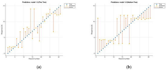
Figure 1.
Results of cross-validation of the model and: (a) «tree (fine tree)» RMSE: 2.8635; R2: 0.62; MAE: 2.2158; (b) «tree (medium tree)» RMSEv: 3.5307; R2: 0.42; MAE: 2.7574.
Medium tree and coarse tree models showed the worst results (R2 was lower than 0.42), and the samples located in the middle of the set showed the highest deviations. Increasing the number of branches in the medium tree and coarse tree methods negatively affected the convergence results; therefore, these models cannot be applied to this type of data.
3.3. The Support Vector Machine
The support vector machine has been actively used with large data sets [21], and previously was successfully applied to build calibration models to predict the physicochemical properties of petroleum systems. The main purpose of this algorithm is to find the most correct position of the line—the flatness that divides the data into classes [51]. When the data are not linearly separable, the SVM transforms original data into a higher dimension using nonlinear mapping to obtain the separating hyperplane. In this work we used the methods of linear SVM, quadratic SVM, cubic SVM, and medium Gaussian SVM.
The linear SVM model (Figure 2) showed the best results; R2 was 0.96, while RMSE was 0.91.
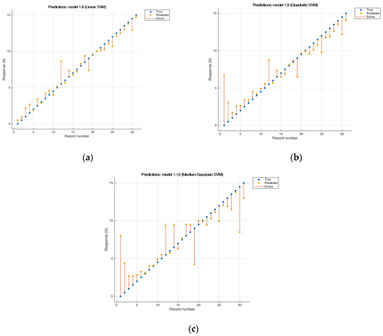
Figure 2.
Results of cross-validation of the model «SVM» (a) linear SVM RMSE: 0.91318; R2: 0.96; MAE: 0.67352, (b) quadratic SVM RMSE: 1.7163; R2: 0.86; MAE: 1.1407; (c) medium Gaussian SVM RMSE: 2.466; R2: 0.72; MAE: 1.6105.
When using the quadratic SVM model (Figure 2b), a negative influence of noise on error during construction appeared, with the largest error observed at the lowest concentrations, perhaps due to the sensitivity of the device at low concentrations and with a small step, which gives the RMSE = 12.214 with a negative R2. In the cubic SVM model, the minimum error was obtained for 28 predictors, but the remaining three predictors made an extremely negative contribution to the overall result. The medium Gaussian SVM model provided the least flexible response function. Interpretation of results for this type of model is difficult. The kernel scale is set to √P. For this model, noise gives a large root mean square error [52].
3.4. Gaussian Regression
In the Gaussian regression method, the response is modeled using a probability distribution over the function space. This regression can be conceptualized as Bayesian linear regression with a kernel, where the kernel parameterization is determined by the choice of covariate/kernel function as well as the data used for prediction. Details of the mathematical algorithm of the methods used are described in [53].
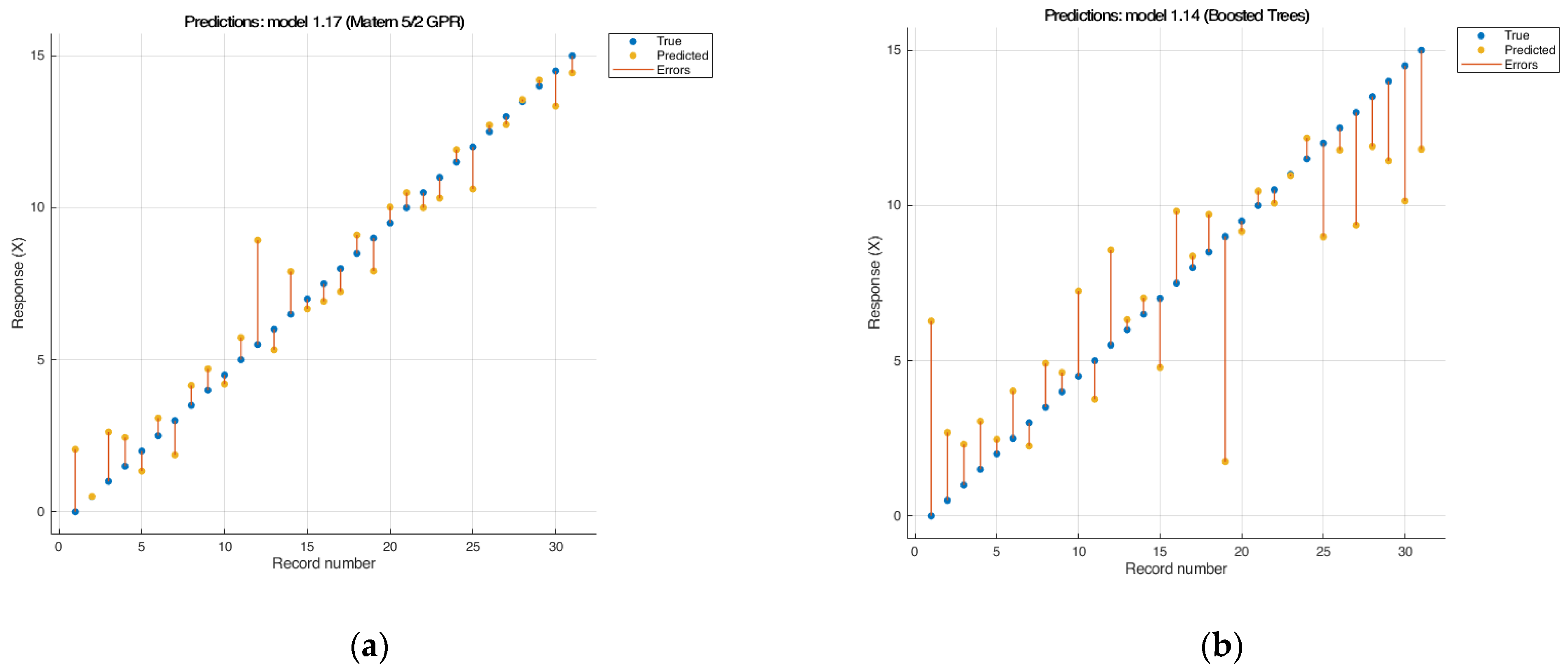
The squared exponential GPR method does not fit the original data array and requires processing. At the same time, the Matern GPR model ensured perfect interpolation (Figure 3a). This model showed very good results: R2 was 0.95 and RMSE 1.034; for this type of model, the noise of the data array is leveled out [54,55].
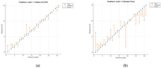
Figure 3.
Results of cross-validation of the model Matern 5.2 GPR и boosted trees: (a) Matern 5.2 GPR RMSE: 1.0348; R2: 0.95; MAE: 0.79655; (b) boosted trees: RMSE: 2.6526; R2: 0.67; MAE: 2.1414.
3.5. Ensembles of Trees
Ensemble tree models are a powerful class of algorithms, which typically exhibit high predictive power because they can model complex dependencies in data. On the one hand, ensembles of trees typically demonstrate high predictive ability because they can model complex dependencies in data, and by combining multiple trees, ensemble trees reduce the risk of overfitting that can occur when using single decision trees. On the other hand, Tree ensembles are usually less interpretable because they are a combination of many trees. However, it is possible to evaluate the importance of features and track which trees contributed to the final prediction [56]. In this work, for creating ensembles of trees models, the following parameters were used: minimum leaf size—8; number of trees—3; number of learners—30; and learning rate—0.1. The boosted trees (Figure 3b) and bagged trees models of ensembles of trees showed unsatisfactory results (R2 < 0.62) and have strong outliers in certain areas, which reduces their value. This unexpected result was an outliner sample from the middle of the calibration set.
3.6. Neural Networks
Neural networks are extremely flexible in training, which allows one to achieve the most approximate result using the maximum possible amount of input data [51,53,54]. In this work, we used fully connected neural networks, which are the most basic type of neural network. They consist of layers of neurons, where each neuron is connected to each neuron of the previous and next layer. Neurons in networks are activated using activation functions such as ReLU, sigmoid, or hyperbolic tangent. Neural networks consist of various layers, including input, hidden and output layers. Two-layer and three-layer neural networks feature additional hidden layers, making them more capable of modeling complex functions and tasks [57]. In this study, the following types of networks were used:
- Neural network: a single-layer neural network with 10 neurons and a final neuron for regression. The ReLU function was used for activation;
- Medium neural network: a single-layer neural network with 25 neurons and a final neuron for regression. The ReLU function was used for activation;
- Wide neural network: a single-layer neural network with 100 neurons and a final neuron for regression. The ReLU function was used for activation;
- Bilayered neural network: a two-layer neural network with 10 neurons on each layer and a final neuron for regression. The ReLU function was used for activation;
- Trilayered neural network: a three-layer neural network with 10 neurons on each layer and a final neuron for regression. The ReLU function was used for activation.
To create the model, 506 points of each of 31 concentrations were used.
However, the neural network methods tested in this work did not show satisfactory results; R2 ranged from 0.64 to 0.76, and RMSE was between 2.2819 and 2.3915. The best results were archived using a trilayered network.
3.7. Summary Results for All Models
Table 2 contains the results of cross-validation for all models.
Among the 21 methods used to build the models, the best results were shown by the SVM (linear SVM) model, where the root mean square error was 0.91; the Gaussian process regression (Matern 5.2 GPR), where the root mean square error was ~1.02; and the Gaussian process regression (rational quadratic) with an RMSE of 1.04.
The models which showed the best results were tested on a test set of samples not included in the training set. The results are presented in Table 3. Testing the method on validation samples showed that the linear SVM model not only has the lowest root mean square error when building a model, but also produces results with an error of no more than 5%.
Table 3.
Results of testing models that showed the best results based on a test sample set.
4. Conclusions
Twenty-one methods of regression analysis of multidimensional data were tested to create a predictive model that allows us to determine the content of n-paraffins in oil using NIR spectroscopy. The best results were obtained using the linear model of the support vector machine (linear SVM), with an RMSE of 0.91; the Gaussian process regression (Matern 5.2 GPR) regression model, the RMSE of which was ~1.02; and the Gaussian process regression (rational quadratic) with an RMSE of 1.04. A chemometric model has been created for determination of n-paraffins content in crude oil, which makes it possible to predict the result with an absolute error of no more than 0.62%. Application of this model in conjunction with an NIR analyzer will enable the determination of the paraffin content in a crude oil stream, which will make it possible to predict and prevent problems associated with paraffin deposits.
Author Contributions
Conceptualization, L.V.I. and V.N.K.; methodology, O.V.P.; software, S.A.S.; validation, S.A.S. and L.V.I.; formal analysis, V.N.K.; investigation, S.A.S.; resources, O.V.P.; writing—review and editing, O.V.P. and V.N.K.; visualization, L.V.I.; supervision, V.N.K. All authors have read and agreed to the published version of the manuscript.
Funding
This research received no external funding.
Data Availability Statement
Data are available from the authors.
Conflicts of Interest
The authors declare no conflict of interest.
References
- Li, W.; Huang, Q.; Wang, W.; Gao, X. Advances and Future Challenges of Wax Removal in Pipeline Pigging Operations on Crude Oil Transportation Systems. Energy Technol. 2020, 8, 1901412. [Google Scholar] [CrossRef]
- Kiyingi, W.; Guo, J.-X.; Xiong, R.-Y.; Su, L.; Yang, X.-H.; Zhang, S.-L. Crude oil wax: A review on formation, experimentation, prediction, and remediation techniques. Pet. Sci. 2022, 19, 2343–2357. [Google Scholar] [CrossRef]
- Lifanov, D.; Orlova, G. Analysis of mechanisms and factors of formation of ASF in cavities of field pipelines and equipment. Trends Dev. Sci. Educ. 2022, 84, 95–97. [Google Scholar]
- Safieva, R. Control of the initial stages of phase formation in oil dispersed systems. Chem. Technol. Fuels Oils 2020, 2, 52–56. [Google Scholar]
- Alnaimat, F.; Ziauddin, M. Wax deposition and prediction in petroleum pipelines. J. Pet. Sci. Eng. 2019, 184, 106385. [Google Scholar] [CrossRef]
- Ruwoldt, J.; Kurniawan, M.; Oschmann, H.-J. Non-linear dependency of wax appearance temperature on cooling rate. J. Pet. Sci. Eng. 2018, 165, 114–126. [Google Scholar] [CrossRef]
- Benamara, C.; Gharbi, K.; Amar, M.N.; Hamada, B. Prediction of Wax Appearance Temperature Using Artificial Intelligent Techniques. Arab. J. Pet. Sci. Eng. 2020, 45, 1319–1330. [Google Scholar] [CrossRef]
- Taheri-Shakib, J.; Shekarifard, A.; Naderi, H. Characterization of the wax precipitation in Iranian crude oil based on Wax Appearance Temperature (WAT): Part 1. The influence of electromagnetic waves. J. Pet. Sci. Eng. 2018, 161, 530–540. [Google Scholar] [CrossRef]
- Kruka, V.R.; Cadena, E.R.; Long, T.E. Cloud-point determination for crude oils. J. Pet. Technol. 1995, 47, 681–687. [Google Scholar] [CrossRef]
- Kok, M.V.; Létoffé, J.-M.; Claudy, P.; Martin, D.; Garcin, M.; Volle, J.-L. Comparison of wax appearance temperatures of crude oils by differential scanning calorimetry, thermomicroscopy and viscometry. Fuel 1996, 75, 787–790. [Google Scholar] [CrossRef]
- Kamari, A.; Rahimzadeh, A.; Mohammadi, A.H.; Ramjugernath, D. Evaluation of wax disappearance temperatures in hydrocarbon fluids using soft computing approaches. Pet. Sci. Technol. 2019, 37, 829–836. [Google Scholar] [CrossRef]
- Hosseinipour, A.; Japper-Jaafar, A.; Yusup, S. Calculations of wax appearance temperature directly from hydrocarbon compositions of crude oil. Int. J. Adv. Appl. Sci. 2019, 6, 90–94. [Google Scholar]
- Eyitayo, S.I.; Lawal, K.A.; Guobadia, K.O.; Ovuru, M.I.; Okoh, O.M.; Yadua, A.U.; Matemilola, S. A comparative evaluation of selected correlations for estimating wax-appearance temperature of crude oils. In Proceedings of the SPE Nigeria Annual International Conference and Exhibition, Virtual, 11–13 August 2020. [Google Scholar]
- Ashmyan, K.D.; Ponomarev, A.K.; Kovaleva, O.V. Consideration of factors affecting the phase state of “paraffins” in reservoir oils. Proc. Sci. Res. Inst. Syst. Res. Rus. Acad. Sci. 2018, 8, 70–73. [Google Scholar]
- GOST 11851-2018; Oil. Methods for the Determination of Paraffins. Federal Agency for Technical Regulation and Metrology: Moscow, Russia, 2018.
- Robustillo, M.D.; Coto, B.; Martos, C.; Espada, J.J. Assessment of Different Methods to Determine the Total Wax Content of Crude Oils. Energy Fuels 2012, 26, 6352–6357. [Google Scholar] [CrossRef]
- Loiko, V.I.; Feshina, E.V. Aspects of the application of BIC spectroscopy. Bull. Mod. Res. 2018, 12, 272–275. [Google Scholar]
- Savelieva, G.V.; Okuneva, E.A. Application of the BIC-spectrometry method in the study of oils and modeling of the TBP curve. Drill. Oil 2018, 11, 30. [Google Scholar]
- Santos, F.D.; Vianna, S.G.T.; Cunha, P.H.P.; Folli, G.S.; de Paulo, E.H.; Moro, M.K.; Romão, W.; de Oliveira, E.C.; Filgueiras, P.R. Characterization of crude oils with a portable NIR spectrometer. Microchem. J. 2022, 181, 107696. [Google Scholar] [CrossRef]
- Wang, S.; Liu, S.; Yuan, Y.; Zhang, J.; Wang, J.; Kong, D. Simultaneous detection of different properties of diesel fuel by near infrared spectroscopy and chemometrics. Infrared Phys. Technol. 2020, 104, 103111. [Google Scholar] [CrossRef]
- Mohammadi, M.; Khorrami, M.K.; Vatani, A.; Ghasemzadeh, H.; Vatanparast, H.; Bahramian, A.; Fallah, A. Rapid determination and classification of crude oils by ATR-FTIR spectroscopy and chemometric methods. Spectrochim. Acta Part A Mol. Biomol. Spectrosc. 2020, 232, 118157. [Google Scholar] [CrossRef]
- Folli, G.S.; Nascimento, M.H.; de Paulo, E.H.; da Cunha, P.H.; Romão, W.; Filgueiras, P.R. Variable selection in support vector regression using angular search algorithm and variance inflation factor. J. Chemom. 2020, 34, e3282. [Google Scholar] [CrossRef]
- Pustokhina, I.; Seraj, A.; Hafsan, H.; Mostafavi, S.M.; Alizadeh, S.M. Developing a robust model based on the gaussian process regression approach to predict biodiesel properties. Int. J. Chem. Eng. 2021, 2021, 5650499. [Google Scholar] [CrossRef]
- Mohammadi, M.; Khorrami, M.K.; Vatani, A.; Ghasemzadeh, H.; Vatanparast, H.; Bahramian, A.; Fallah, A. Genetic algorithm based support vector machine regression for prediction of SARA analysis in crude oil samples using ATR-FTIR spectroscopy. Spectrochim. Acta Part A Mol. Biomol. Spectrosc. 2021, 245, 118945. [Google Scholar] [CrossRef]
- Mat-Desa, W.N.S.; Ismail, D.; NicDaeid, N. Classification and source determination of medium petroleum distillates by chemometric and artificial neural networks: A self-organizing feature approach. Anal. Chem. 2011, 83, 7745–7754. [Google Scholar] [CrossRef]
- Ou, F.; van Klinken, A.; Ševo, P.; Petruzzella, M.; Li, C.; van Elst, D.M.J.; Hakkel, K.D.; Pagliano, F.; van Veldhoven, R.P.J.; Fiore, A. Handheld NIR Spectral Sensor Module Based on a Fully-Integrated Detector Array. Sensors 2022, 22, 7027. [Google Scholar] [CrossRef] [PubMed]
- Ozaki, Y.; Genkawa, T.; Futami, Y. Near-Infrared Spectroscopy; Gakkai Shuppan Center: Tokyo, Japan, 1996; p. 68. [Google Scholar]
- Jacobi, H.F.; Moschner, C.R.; Hartung, E. Use of near infrared spectroscopy in online-monitoring of feeding substrate quality in anaerobic digestion. Bioresour. Technol. 2011, 102, 4688–4696. [Google Scholar] [CrossRef]
- Zhang, W.; Kasun, L.C.; Wang, Q.J.; Zheng, Y.; Lin, Z. A Review of Machine Learning for Near-Infrared Spectroscopy. Sensors 2022, 22, 9764. [Google Scholar] [CrossRef] [PubMed]
- Kim, M.; Lee, Y.H.; Han, C. Real-time classification of petroleum products using near-infrared spectra. Comput. Chem. Eng. 2000, 24, 513–517. [Google Scholar] [CrossRef]
- Garmarudi, A.B.; Khanmohammadi, M.; Fard, H.G.; de la Guardia, M. Origin based classification of crude oils by infrared spectrometry and chemometrics. Fuel 2019, 236, 1093–1099. [Google Scholar] [CrossRef]
- Baird, Z.S.; Oja, V. Predicting fuel properties using chemometrics: A review and an extension to temperature dependent physical properties by using infrared spectroscopy to predict density. Chemom. Intell. Lab. Syst. 2016, 158, 41–47. [Google Scholar] [CrossRef]
- de Paula Pedroza, R.H.; Nicácio, J.T.N.; dos Santos, B.S.; de Lima, K.M.G. Determining the kinematic viscosity of lubricant oils for gear motors by using the near infrared spectroscopy (NIRS) and the wavelength selection. Anal. Lett. 2013, 46, 1145–1154. [Google Scholar] [CrossRef]
- Zhu, L.; Lu, S.H.; Zhang, Y.H.; Zhai, H.L.; Yin, B.; Mi, J.Y. An effective and rapid approach to predict molecular composition of naphtha based on raw NIR spectra. Vib. Spectrosc. 2020, 109, 103071. [Google Scholar] [CrossRef]
- Araujo, A.M.; Santos, L.M.; Fortuny, M.; Melo, R.L.F.V.; Coutinho, R.C.C.; Santos, A.F. Evaluation of water content and average droplet size in water-in-crude oil emulsions by means of near-infrared spectroscopy. Energy Fuels 2008, 22, 3450–3458. [Google Scholar] [CrossRef]
- Ferreira, L.; Machado, N.; Gouvinhas, I.; Santos, S.; Celaya, R.; Rodrigues, M.; Barros, A. Application of Fourier transform infrared spectroscopy (FTIR) techniques in the mid-IR (MIR) and near-IR (NIR) spectroscopy to determine n-alkane and long-chain alcohol contents in plant species and faecal samples. Spectrochim. Acta Part A Mol. Biomol. Spectrosc. 2022, 280, 121544. [Google Scholar] [CrossRef] [PubMed]
- Breiman, L.; Friedman, J.H.; Olshen, R.A.; Stone, C.J. Classification and Regression Trees; Taylor and Francis: New York, NY, USA, 1984; 368p. [Google Scholar]
- Osuna, E.; Freund, R.; Girosit, F. Training support vector machines: An application to face detection. In Proceedings of the Proceedings of IEEE Computer Society Conference on Computer Vision and Pattern Recognition, San Juan, PR, USA, 17–19 June 1997; pp. 130–136. [Google Scholar]
- Rasmussen, C.E.; Williams, C.K.I. Gaussian Processes for Machine Learning; MIT Press: Cambridge, MA, USA, 2006; 248p. [Google Scholar]
- Gladkov, L.A.; Kureychik, V.V.; Kureychik, V.M. Genetic Algorithms; Fizmatlit: Moscow, Russia, 2010; p. 317. [Google Scholar]
- Goodfellow, Y.; Bengio, I.; Kurvill, A. Deep Learning, 2nd ed.; DMK Press: Moscow, Russia, 2018; p. 652. [Google Scholar]
- Römer, M. Investigating Physical Properties of Solid Dosage Forms During Pharmaceutical Processing: Process Analytical Applications of Vibrational Spectroscopy. Ph.D. Thesis, University of Helsinki, Helsinki, Finland, 2008. [Google Scholar]
- Hammami, A.; Ratulowski, J.; Coutinho, J.A.P. Cloud Points: Can We Measure or Model Them? Pet. Sci. Technol. 2003, 21, 345–358. [Google Scholar] [CrossRef]
- Chicco, D.; Warrens, M.J.; Jurman, G. The Coefficient of Determination R-Squared Is More Informative Than SMAPE, MAE, MAPE, MSE, and RMSE in Regression Analysis Evaluation. PeerJ Comput. Sci. 2021, 7, e623. [Google Scholar] [CrossRef]
- Deisenroth, M.P.; Faisal, A.; Cheng, S.O. Mathematics for Machine Learning; Cambridge University Press: Cambridge, UK, 2015; p. 405. [Google Scholar]
- Demidenko, E.Z. Linear and Nonlinear Regression; Finance and Statistics: Moscow, Russia, 1981; p. 302. [Google Scholar]
- Bauer, D.J.; Curran, P.J. Probing Interactions in Fixed and Multilevel Regression: Inferential and Graphical Techniques. Multivar. Behav. Res. 2005, 40, 373–400. [Google Scholar] [CrossRef] [PubMed]
- Cadet, F. Quantitative Analysis, Infrared. Encyclopedia of Analytical Chemistry. 2012. [Google Scholar]
- Rokach, L.; Maimon, O. Data Mining with Decision Trees: Theory and Applications, 2nd ed.; World Scientific Pub Co Inc: Singapore, 2014. [Google Scholar]
- Hastie, T.; Tibshirani, R.; Friedman, J.H. Additive Models, Trees, and Related Methods. In The Elements of Statistical Learning: Data Mining, Inference, and Prediction; Springer: New York, NY, USA, 2009; p. 758. [Google Scholar]
- Smola, A.J.; Schölkopf, B. A tutorial on support vector regression. Stat. Comput. 2004, 14, 199–222. [Google Scholar] [CrossRef]
- Hastie, T.; Tibshirani, R.; Friedman, J.H. Overview of Supervised Learning. In The Elements of Statistical Learning: Data Mining, Inference, and Prediction; Springer: New York, NY, USA, 2008; p. 134. [Google Scholar]
- Rasmussen, C.E.; Williams, C.K.I. Average-Case Learning Curves. In Gaussian Processes for Machine Learning; MIT Press: Cambridge, MA, USA, 2006; p. 159. [Google Scholar]
- Nielsen, M.A. Neural Networks and Deep Learning; Determination Press: San Francisco, CA, USA, 2015; p. 216. [Google Scholar]
- MacKay, D.J.C. Information Theory, Inference, and Learning Algorithms; Cambridge University Press: Cambridge, UK, 2003; p. 628. [Google Scholar]
- Freund, Y.; Schapire, R.E. A decision-theoretic generalization of on-line learning and an application to boosting. J. Comput. Syst. Sci. 1997, 55, 119–139. [Google Scholar] [CrossRef]
- Wu, Y.C.; Feng, J.W. Development and application of artificial neural network. Wirel. Pers. Commun. 2018, 102, 1645–1656. [Google Scholar] [CrossRef]

Disclaimer/Publisher’s Note: The statements, opinions and data contained in all publications are solely those of the individual author(s) and contributor(s) and not of MDPI and/or the editor(s). MDPI and/or the editor(s) disclaim responsibility for any injury to people or property resulting from any ideas, methods, instructions or products referred to in the content. |
© 2023 by the authors. Licensee MDPI, Basel, Switzerland. This article is an open access article distributed under the terms and conditions of the Creative Commons Attribution (CC BY) license (https://creativecommons.org/licenses/by/4.0/).