Fuzzy Gain Scheduling of the Fractional-Order PID Controller for a Continuous Stirred-Tank Reactor Process

Abstract

In most chemical industries, continuous stirred-tank reactors (CSTRs) are essential for the production of chemicals. The CSTR process is highly nonlinear and has both stable and unstable equilibrium points. Control system engineers face a difficult issue when designing a single controller for temperature control in both stable and unstable areas. Due to these problems, implementing the conventional proportional-integral-derivative (PID) controller may lead to instability in controlled variables. Therefore, in this paper, the entire operating region is divided into three regions. The fractional-order PID controller as a local controller is designed in each operating region to control the temperature, and its parameters are tuned with a genetic algorithm by minimizing the integral of absolute error and control input change with a weighting factor. Then, a fuzzy gain scheduling scheme based on the Tagaki-Sugno fuzzy model is used to properly interpolate the outputs of the local controllers. A set of simulations are carried out to demonstrate the effectiveness of the proposed controller, and its performance is compared with that of an adaptive nonlinear controller and fuzzy gain scheduling of the PID controller.

1. Introduction

A continuous stirred-tank reactor (CSTR) is the commonly adopted and key reactor in the chemical industry due to its potential safety problems. In the case of an exothermic reaction, the reactor releases the heat, and its temperature increases very fast. This affects the formation of the product as well as the safety and lifetime of the reactor. CSTRs exhibit different dynamic characteristics depending on the operating conditions and have stable and unstable equilibrium states with rapidly changing behaviors in the vicinity of an unstable equilibrium state [1,2,3,4,5].

Over the past decades, a number of methods relevant to the temperature control of non-isothermal CSTR processes and their applications have been proposed in the literature, such as proportional-integral-derivative (PID) control [6,7,8], linear quadratic regulator (LQR) [9,10], nonlinear control [11,12,13,14], fuzzy control [15,16], fractional-order PID (FOPID) control [17,18,19,20,21], and other methods incorporating evolutionary algorithms and gain scheduling [22]. In the literature [6], non-isothermal CSTR and PID control were used for process simulation, and the stability of the reactor at different tuning points and disturbances was checked. Baruah et al. [7] and Boobalan et al. [8] designed a PID controller for the temperature stabilization of CSTRs based on an evolutionary algorithm, and the results were compared for set-point tracking and disturbance rejection. Although the conventional PID controller has been successfully employed for CSTR process control and the fixed-parameter PID controller can achieve desired performance under the planned operating point, there have been some difficulties when the operating point changes. In the literature [9,10], a linear quadratic regulator (LQR) was designed based on a linearized model to control the temperature of the CSTR process, and the responses were compared with those of a conventional PID controller. The weighting matrices Q and R were chosen with the trial-and-error method in [9] and by using a bacterial foraging algorithm in [10].

In recent decades, many research efforts have been devoted to combining existing control platforms with nonlinear techniques [11,12,13,14] and/or fuzzy theory [15,16]. The designed sliding mode control (SMC) for a CSTR was performed where the process was controlled by combining a sliding mode controller with a disturbance observer [11]. Sinha et al. [12] used SMC using triggered techniques to control the temperature of the CSTR process. As another approach, feedback linearization was employed for applying optimal control to the CSTR process in [13] and for product concentration control in [14]. In these works, the nonlinear process was converted to a linearized model through the use of nonlinear coordinate transformations, and a LQR controller was designed for the linearized model to achieve the nonlinear feedback control law. In Lakshmi et al. [15], the response from the fuzzy logic controller was compared with those of conventional PI and PID controllers. In Prabhu et al. [16], a fuzzy logic controller was used for the temperature control of the non-isothermal CSTR process. The response was compared with the PID controller.

One of the existing and powerful approaches for controlling nonlinear processes is gain scheduling, which has been widely applied in fields such as aerospace and process control. Gain scheduling interpolates between a set of local controllers derived for corresponding linearized models at several operating points [22]. Despite the widespread application of gain scheduling approaches, if scheduling variables are contaminated with considerable noise, the classical approach cannot provide a satisfactory response. A number of studies have been formulated on the combination of gain scheduling and fuzzy theory for the CSTR process control [23,24,25,26]. In Ranjan’s work [23], a gain-scheduled composite nonlinear feedback controller was implemented for CSTR. This strategy implements linear and nonlinear feedback components and then combines the linear and nonlinear feedback components. Kim et al. [24] proposed a combination of the two-degree-of-freedom PID controller with the anti-windup technique and a fuzzy gain scheduler for its application to CSTR. A set of controller parameters were expressed as functions of the gain scheduling variable using a set of ‘if-then’ fuzzy rules, which were of Sugeno’s form. In Bingi et al. [25], a gain-scheduled set-point weighted PID controller for an unstable CSTR system was used. In that work, the fuzzy gain scheduling was used as an adaptation mechanism for tuning the set-point weighted PID controller parameters. Fábregas et al. [26] implemented a control strategy using gain scheduling that allows the calculation of the PID controller by using the fuzzy inference system in real-time.

In the last two decades, as fractional calculus proposed by Podlubny et al. [17] in 1997 regained interest from scientists and engineers, it has been applied in many fields. The fractional-order PID (FOPID) controller introduces the non-integer order of I-term and D-term in its structure at the expense of complexity. Unlike the conventional PID controller, the FOPID controller has two more parameters, that is, integral and derivative orders. These give the benefits of additional tuning flexibility, and the FOPID controller is effective in minimizing the effect of disturbances and set-point change problems [17,18,19,20,21].

In this paper, we deal with the design of a fuzzy gain-scheduled FOPID controller for a CSTR process by combining FOPID control and fuzzy gain scheduling. The dynamic characteristics of the CSTR process are analyzed throughout the entire range of operating conditions. The operation is categorized into three regions (low, middle, and high) according to the equilibrium points of the CSTR process. Then, the FOPID controller as the local controller is designed, and its parameters are optimally tuned using a genetic algorithm (GA) by minimizing the integral of absolute error and control input change with a weighting factor. Finally, a global controller is implemented through fuzzy gain scheduling of the three local FOPID controllers. The effectiveness of the proposed method is assessed through simulation according to a set of scenarios. The performance of the proposed controller is compared with those of the fuzzy gain-scheduled PID controller tuned with a GA and an adaptive controller.

The primary contributions of this paper are as follows:

-

The dynamic characteristics of the highly nonlinear CSTR process were analyzed, and based on these characteristics, the entire operating range was divided into three regions.

-

Three local FOPID controllers were designed, one for each of the three operating regions.

-

For controller design, both the integral of absolute error (IAE) and control input change with weighting factor were simultaneously used as evaluation criteria.

-

A fuzzy gain scheduling technique was employed to integrate the three local controllers.

The paper’s structure is as follows: In Section 2, the modeling of the highly nonlinear CSTR process is explained, and its dynamic characteristics are analyzed. Section 3 describes the fuzzy gain scheduling of the proposed FOPID controller. To do this, it begins with a brief explanation of fractional calculus, followed by an introduction to the transfer function of the local FOPID controller and an explanation of the tuning method for these local FOPID controllers. It then elaborates on the fuzzy gain scheduling to combine the individual local controllers. In Section 4, simulations are carried out on the nonlinear CSTR process, and the performance of the proposed controller is compared with that of traditional fuzzy gain scheduling integer-order PID controller and adaptive controller. Finally, Section 5 concludes the paper.

2. Modeling of a CSTR Process

CSTR is a key reactor used for pyrolytic reaction and catalyst-using polymer synthesis in chemical industries [1,2,3,4,5]. It is highly nonlinear and time-varying, and it is difficult to analyze and control. In order to maintain an optimal condition in which a perfect reaction occurs within the reactor, the internal temperature needs to be kept constant along with strong agitation. Figure 1 shows the schematic diagram of a CSTR process.

In Figure 1, C_f, T_f, F_f and C, T, F are reactant concentration [mol/m³], reactor temperature [K] and flow rate [m³/sec] at the inlet and outlet of reactant, respectively; T_cf, F_cf and T_c, F_c are the temperature and flow rate at the inlet and outlet of cooling water, respectively.

2.1. Dimensionless State Space Model

Consider the case of a single irreversible exothermic reaction with A → B. Assuming a well-stirred solution with constant volume and constant physical parameters, the dimensionless dynamic material and energy balances are given by [1,2].

$${\dot{x}}_1(t)=-x_1(t)+D_a[1-x_1(t)]\exp [\frac{x_2(t)}{1+x_2(t)/\gamma }]+d_1(t)$$

(1a)

$${\dot{x}}_2(t)=-(1+\beta )x_2(t)+H{D}_a[1-x_1(t)]\exp [\frac{x_2(t)}{1+x_2(t)/\gamma }]+\beta u(t)+d_2(t)$$

(1b)

$$y(t)=x_2(t)$$

(1c)

where D_a is the Damökhler number, H is the heat of reaction, β is the heat transfer coefficient, V is the volume of CSTR [m³], $\gamma =E/R{T}_f$, E is the activation energy [cal/mol] and R is the gas constant [cal/mol-K]. d₁ and d₂ are the disturbances in the reactant concentration and feed temperature, respectively. It is assumed that disturbances are stepwise. x₁, x₂, u, and t are the dimensionless reactant concentration, reactant temperature, jacket coolant temperature, and time, respectively, defined as

$$x_1=\frac{C_f-C}{C_f}, x_2=\frac{T-T_f}{T_f}\gamma , u=\frac{T_{cf}-T_f}{T_f}\gamma , and t=t^{\prime }\frac{F_f}{V}$$

(2)

where t′ denotes the actual time in seconds.

Equation (3) shows the relationship between the actual reactor temperature T at the outlet and the dimensionless variable x₂.

$$T=(1+\frac{x_2}{\gamma })T_f$$

(3)

2.2. Steady-State Characteristics

Applying typical parameter values of D_a = 0.072, H = 8, β = 0.3, and γ = 20 to Equation (1) gives the steady-state behavior of the CSTR process. Figure 2 depicts the curves of x₁(t) and x₂(t) vs. u(t) in the steady-state as well as three equilibrium states: x_a = [0.1440, 0.8860]^T, x_b = [0.4472, 2.7517]^T, and x_c = [0.7646, 4.7050]^T. The top x_c and the bottom x_a denote stable equilibrium states, while the middle x_b denotes an unstable equilibrium state. Assuming that the CSTR will be operated between y = 0 and 6, the curve can be categorized into three regions (low, middle, and high) by the equilibrium points as the boundaries. It can be obvious that the CSTR clearly exhibits highly nonlinear characteristics in the vicinity of the middle region, having multiple outputs for the same control input.

This characteristic indicates that a fixed-parameter controller can have difficulty in controlling, i.e., possibly degrading the quality of the product. More advanced methods, such as adaptive control or a gain scheduling scheme are required instead.

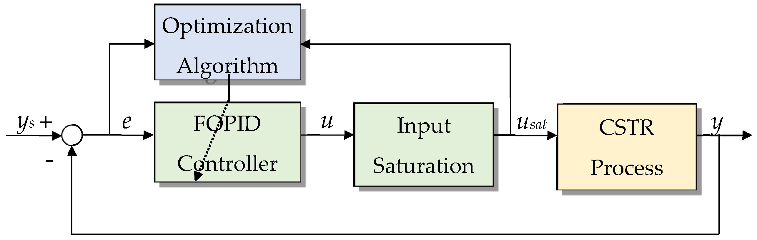
3. Fuzzy Gain Scheduling of the FOPID Controller

As seen in the preceding section, the characteristics of the CSTR depend highly on the operation region. Therefore, in this section, fractional-order PID (FOPID) controllers as local controllers are designed, and then the global controller is achieved by using fuzzy gain scheduling to cope with the full operation changes.

3.1. Fractional Calculus

Fractional calculus is a generalization of the integration and differentiation to the non-integer order operator. The integral-differential operator D^α is defined as

$$D^{\alpha }=\left\{\begin{array}{cc}\frac{d^{\alpha }}{dt},& \alpha >0\\ 1,& \alpha =0\\ {\displaystyle {\int }_0^t{(d\tau )}^{-\alpha }},& \alpha <0\end{array}\right.$$

(4)

where α ∈ R is the fractional order.

Several definitions for the fractional operator D^α, such as the Grünwald-Letnikov definition, the Caputo definition, and the Riemann-Liouville (R-L) definition can be found in the literature [17,18]. The R-L fractional integration and differentiation are defined as

$$D^{-\alpha }f(t)=\frac{1}{\Gamma (\alpha )}{\displaystyle {\int }_0^t{(t-\tau )}^{\alpha -1}f(\tau )d\tau }$$

(5)

$$D^{\alpha }f(t)=\frac{1}{\Gamma (1-\alpha )}\frac{d}{dt}{\displaystyle {\int }_0^t{(t-\tau )}^{-\alpha }f(\tau )d\tau }$$

(6)

where Γ denotes Euler’s gamma function. The Laplace transform of the R-L fractional integration and differentiation are given by

$$L\left\{D^{-\alpha }f(t)\right\}=s^{-\alpha }F(s)$$

(7)

$$L\left\{D^{\alpha }f(t)\right\}=s^{\alpha }F(s)-{\left.D^{\alpha -1}f(t)\right|}_{t=0}$$

(8)

3.2. FOPID Controllers as Local Controller

Based on fractional calculus, the mathematical equation of a FOPID controller is given by

$$u(t)=K_{p}e(t)+K_i{D}^{-\lambda }e(t)+K_d{D}^{\mu }e(t)$$

(9)

where e(t) is the error as the difference between the set-point and the output, and u is the control input; K_p, K_i and K_d are the proportional, integral, and derivative gains, respectively; λ and µ are the real number orders satisfying 0 < λ, µ < 2. Note that if λ = µ = 1, as we can see, the standard PID form is obtained. This expansion provides a more flexible controller design.

The transfer function of Equation (9) is given by

$$\frac{U(s)}{E(s)}=K_p+\frac{K_i}{s^{\lambda }}+K_d{s}^{\mu }$$

(10)

As mentioned previously, the operation is divided into three regions and three FOPID controllers are employed for the local controllers at each region. On the other hand, when a large set-point is abruptly applied, an excessive controller output exceeds the input range of the actuator, so an input saturator is assumed to limit this within the range [–5, 5].

3.3. Tuning of the FOPID Controller

As seen in Equation (10), each FOPID controller has five user-defined parameters (K_p, K_i, K_d, λ and µ). These parameters should be tuned by carefully considering the operating range of the CSTR process, so that the closed-loop control system with the input saturation maintains the desired performance. A set of tuning procedures are used to obtain the optimal parameters of the three local controllers based on the nonlinear model in Equation (1). D_a, γ, H, and β are set to the nominal values, and during tuning, the disturbances are assumed to be zero. Figure 3 depicts the offline tuning process of the FOPID controller at each operating point using an optimization algorithm.

At this time, the following evaluation called the integral of absolute error and control input change with weighting factor (IAEU) is used as a quantitative measure of the system performance to obtain the FOPID parameters:

$$\mathrm{IAEU}={\displaystyle {\int }_0^{\infty }(\left|e(t)\right|+w\left|\mathsf{\Delta }u(t)\right|)dt}$$

(11)

where e(t) is the error with e(t) = y_s(t) − y(t), Δu(t) is the deviation of control input from the steady-state value u₀ with Δu(t) = u_sat(t) − u₀, and w is the weighting factor. This performance index is particularly useful for suppressing unnecessarily excessive control effort at the expense of a slower response by changing w. A GA adjusts the parameters of the FOPID controller so that IAEU is minimized. The searching procedure of the GA algorithm is described as Algorithm 1.

Algorithm 1. Genetic Algorithm

Initialize a population randomly;   Evaluate individuals in the population using Equation (11); While < termination condition not met > {    Select individuals based on their fitness;    Crossover individuals;    Mutate individuals;    Evaluate individuals in the new population using Equation (11); } Output the best solution;

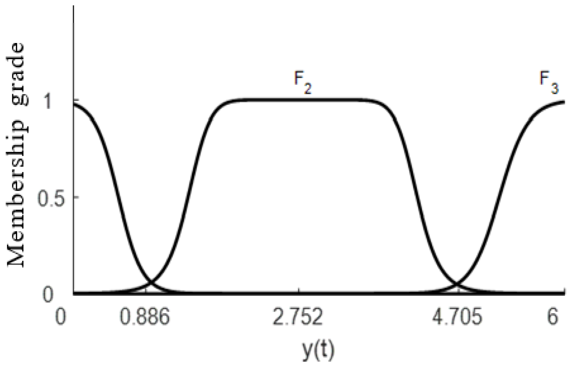
3.4. Fuzzy Gain Scheduling

Gain scheduling is one of the commonly used and powerful approaches for controlling nonlinear processes whose dynamics change from one operating point to another. If the local controller is designed in the vicinity of each operating point of the process and its parameters are properly tuned, the next step is to interpolate between a set of the local controllers using a scheduling variable, such as a measurable output to achieve the global (gain-scheduled) controller. Then, the global controller has the potential of responding flexibly during transitions between operating points. Despite the widespread application of gain scheduling approaches, if the scheduling variable is contaminated with considerable noise, the classical approach cannot provide a satisfactory response.

For these reasons, fuzzy gain scheduling is considered in this study. The fuzzy sets, linguistic rules, and approximate reasoning provide a flexible and clear method of gain scheduling. To identify the current operating region on the CSTR process, the output y (=x₂) is used as scheduling variable. Then the fuzzy gain scheduler selects the controller according to the scheduling variable. Three fuzzy sets are defined over the output variable. Their membership function shapes are shown in Figure 4.

The left and right membership functions are the sigmoid functions, and the middle membership function is the generalized bell function. Based on the Takagi-Sugeno (T-S) method of fuzzy inference, the fuzzy gain scheduler is given by a set of fuzzy rules of the form

$$\mathrm{Rule} 1: \mathrm{if} y\left(t\right) \mathrm{is} F_1, \mathrm{then} u_1(t)=K_p{}_{1}e(t)+K_i{}_1{D}^{-{\lambda }_1}e(t)+K_d{}_1{D}^{{\mu }_1}e(t)$$

(12a)

$$\mathrm{Rule} 2: \mathrm{if} y\left(t\right) \mathrm{is} F_2, \mathrm{then} u_2(t)=K_{p2}e(t)+K_i{}_2{D}^{-{\lambda }_2}e(t)+K_d{}_2{D}^{{\mu }_2}e(t)$$

(12b)

$$\mathrm{Rule} 3: \mathrm{if} y\left(t\right) \mathrm{is} F_3, \mathrm{then} u_3(t)=K_{p3}e(t)+K_{i3}{D}^{-{\lambda }_3}e(t)+K_{d3}{D}^{{\mu }_3}e(t)$$

(12c)

where y(t) and u_i(t) (i = 1, 2, 3) denote the input and output variables of the fuzzy inference system, respectively; F_i (i = 1, 2, 3) are fuzzy sets; K_pj, K_ij, K_dj, λ_j, and μ_j (j = 1, 2, 3) are the parameters of the local FOPID controllers. Then, the inferred result is expressed by

$$u(t)={\displaystyle \sum _{i=1}^3{\alpha }_i{u}_i(t)}/{\displaystyle \sum _{i=1}^3{\alpha }_i}$$

(13)

where α_i is the truth value of the ith rule with α_i = F_i(y) ≥ 0. As can be seen from Figure 4, by allowing appropriate overlap between adjacent membership functions, ${\displaystyle \sum _{i=1}^3{\alpha }_i}>0$ is always maintained for any value of y.

Figure 5 shows the schematic diagram of the fuzzy gain-scheduled FOPID control system.

4. Simulation Results

In this section, a simulative study is performed on the CSTR model in Equation (1) with the parameter values of D_a = 0.072, H = 8, β = 0.3, and γ = 20 to illustrate the effectiveness of the proposed method. The FOPID controller is implemented using the FOMCON package [27]. The responses of the fuzzy gain-scheduled FOPID controller are compared with those of the fuzzy gain-scheduled PID controller and the adaptive controller [28]. For convenience, the method in which the FOPID controllers are fuzzy gain scheduled is abbreviated as ‘FG-FOPID’, and the method in which the PID controllers are fuzzy gain scheduled is abbreviated as ‘FG-PID’.

In the case of the FG-PID controller, the same tuning method and fuzzy gain scheduling as applied in the FG-FOPID controller are accepted, and the parameters of the local PID controller are tuned by another GA such that the evaluation function of Equation (11) is minimized. The simulation of the FG-PID controller is also conducted under the schematic diagram similar to Figure 5. However, the difference is that the three local controllers use the signals provided by integer-order integrator and differentiator. On the other hand, for obtaining the response of the Chen’s adaptive controller, η = 0.2, m = 5, and sign(∂y/∂x) = 1 are set as in [28].

Although the FOPID and PID controllers are tuned to favor set-point tracking, simulations on set-point tracking as well as disturbance rejection are performed on the closed-loop system as shown in Figure 5.

The five parameters of the FOPID controller were searched between the lower bound [0 0 0 0 0] and the upper bound [50 30 30 2 2]. The three parameters of the PID controller were searched between [0 0 0] and [50 30 30]. The weight factor w was set to 0.1. Optimally tuned parameters are summarized in

Table 1. Tuned parameters of the FOPID and PID controllers.

Local Controllers	Parameters
	Kp	Ki	Kd	λ	μ
FOPID 1	36.547	3.317	14.189	0.905	0.539
FOPID 2	30.497	4.456	13.611	0.347	0.582
FOPID 3	17.339	4.067	11.862	0.901	0.629
PID 1	6.516	2.015	3.179	-	-
PID 2	3.962	0.280	2.629	-	-
PID 3	5.841	2.693	2.561	-	-

.

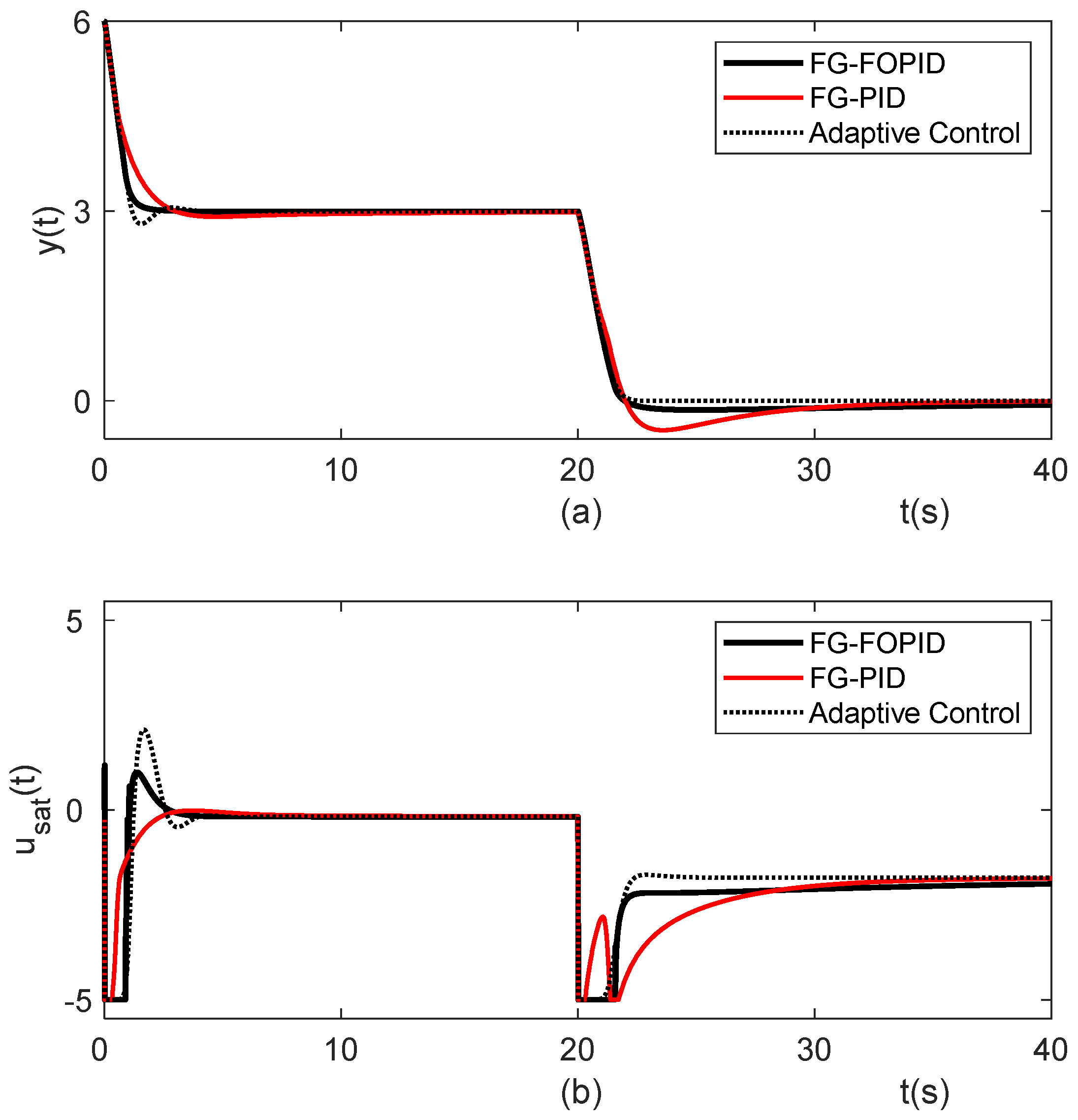
4.1. Set-Point Tracking Test

In order to compare the set-point tracking performance of the three methods, the following four scenarios are considered.

• Case 1: The initial output y is set to 0 with all initial settings. The set-point y_s is changed stepwise from 0 to 3 at 0 s and again changed from 3 to 6 at 20 s.
• Case 2: The initial output y is set to 6 with all initial settings. y_s is changed from 6 to 3 at 0 s and again changed from 3 to 0 at 20 s.
• Case 3: The initial output y is set to 0 with all initial settings. y_s is changed from 0 to 2.7517 (unstable equilibrium) at 0 s and again changed to 0 at 20 s.
• Case 4: The initial output y is set to 6 with all initial settings. y_s is changed from 6 to 2.7517 (unstable equilibrium) at 0 s and again changed to 6 at 20 s.

The set-point tracking performance is measured in terms of the rise time (t_r), percentage overshoot (M_p), settling time (t_s), and IAE [29] defined as

$$IAE={\displaystyle {\int }_0^{\infty }\left|e(t)\right|dt}$$

(14)

Figure 6 shows the response comparison of the output and saturated control input executed according to the scenario of Case 1. It can be seen from Figure 6 that the FG-FOPID controller shows a better performance with a smaller overshoot for the first setpoint change interval of time, but for the second setpoint change, the adaptive controller shows a faster response at the expense of a larger overshoot than the others. The performance results of the three methods for Case 1 are summarized in

Table 2. Set-point tracking performance for Case 1.

Methods	ys = 0 → 3
	tr	Mp	ts	IAE
FG-FOPID	1.707	0.841	1.791	3.068
FG-PID	2.602	10.168	10.420	5.962
Adaptive control	1.528	13.772	2.706	3.020
	ys = 3 → 6
FG-FOPID	0.877	9.052	8.765	4.020
FG-PID	1.075	8.274	4.182	2.820
Adaptive control	0.715	9.580	2.016	1.963

. As can be seen in the table, when y_s is increased from 0 to 3, the FG-FOPID controller has a smaller overshoot with t_s of 1.79 s and IAE of 3.07, whereas the FG-PID and adaptive controllers have an overshoot of 10.2% and 13.8% with a longer t_s, respectively. When y_s is increased from 3 to 6, the FG-FOPID controller has a longer t_s of 8.77 s and a larger IAE of 4.02 than the others.

The set-point tracking responses of the CSTR closed-loop system for Case 2 are shown in Figure 7. The quantitative performances are compared in

Table 3. Set-point tracking performance for Case 2.

Methods	ys = 6 → 3
	tr	Mp	ts	IAE
FG-FOPID	1.230	0.303	1.299	1.905
FG-PID	2.240	2.958	2.302	3.181
Adaptive control	1.011	6.738	1.839	1.866
	ys = 3 → 0
FG-FOPID	1.548	4.767	1.650	4.332
FG-PID	1.749	15.470	8.904	5.389
Adaptive control	1.644	0	1.751	2.522

. For the first part of the responses, the FG-FOPID controller provides an overshoot M_p of 0.30% and a settling time t_s of 1.30 s, which are better than the others. For the second part of the responses, the adaptive control shows better performance in the case of overshoot and IAE as compared to those of the others. From all points of view, the FG-FOPID controller provides better performance.

Figure 8 and Figure 9 show the set-point tracking responses for Cases 3 and 4, and their comparative performances are summarized in

Table 4. Set-point tracking performance for Case 3.

Methods	ys = 0 → 2.7517
	tr	Mp	ts	IAE
FG-FOPID	1.647	0.643	1.724	2.501
FG-PID	2.762	7.598	8.517	4.896
Adaptive control	1.460	10.377	2.512	2.507
	ys = 2.7517 → 0
FG-FOPID	1.865	0	1.642	2.487
FG-PID	1.959	8.611	6.761	3.992
Adaptive control	1.591	0	1.688	2.200

and

Table 5. Set-point tracking performance for Case 4.

Methods	ys = 6 → 2.7517
	tr	Mp	ts	IAE
FG-FOPID	1.302	0.489	1.376	2.296
FG-PID	2.227	4.962	2.294	4.240
Adaptive control	1.093	6.352	1.938	2.162
	ys = 2.7517 → 6
FG-FOPID	1.874	0	1.968	2.506
FG-PID	1.125	8.119	4.030	3.259
Adaptive control	0.760	11.649	2.014	2.274

. It can be seen from the figures and the tables that the overall performance of the proposed method is better than that of the others. The proposed method has M_p = 0.64% and t_s = 1.72 s for the first part of Case 3 and M_p = 0% and t_s = 1.64 s for the second part of Case 3, as well as M_p = 0.49% and t_s = 1.38 s for the first part of Case 4 and M_p = 0% and t_s = 1.97 s for the second part of Case 4.

4.2. Disturbance Rejection Test

Disturbances are, in general, unpredictable and unmeasurable and influence the system performance significantly in real applications. Therefore, it is of great importance to check the disturbance rejection performance of the closed-loop system in the presence of disturbances. In this simulation, two disturbances, inlet concentration d₁ and inlet temperature d₂, are assumed. To assess the disturbance rejection performance of the three methods, simulations are conducted based on two scenarios.

• Case 5: The initial output is kept at the set-point of 0.866 (stable equilibrium). Stepwise, disturbance d₁ is changed from 0 to 0.1, while d₂ is changed from 0 to −0.1 at 0 s.
• Case 6: The initial output is kept at the set-point of 0.866 (stable equilibrium). Stepwise, disturbance d₁ is changed from 0 to −0.1, while d₂ is changed from 0 to 0.1 at 0 s.

Similar to the case of the set-point tracking performance test, the disturbance rejection performance is measured in terms of peak time (t_peak), perturbance peak (M_peak), recovery time (t_rcy), and IAE [29].

Figure 10 shows the disturbance rejection responses for Cases 5 and 6. It can be seen in the figures that the responses of the three methods initially deviate from the set-point due to disturbance changes, and after a while, they recover to the set-point. The FG-FOPID controller has the smallest deviation from the output, but it shows slower recovery instead. This is because the controller is tuned to favor set-point tracking.

Table 6. Disturbance rejection performance for Cases 5 and 6.

Scenario	Methods	Performance Indices
		tpeak	Mpeak	trcy	IAE
Case 5	FG-FOPID	3.153	0.015	136.49	0.812
	FG-PID	2.410	0.069	20.245	0.553
	Adaptive control	0.740	0.027	4.673	0.059
Case 6	FG-FOPID	3.232	0.015	135.60	0.790
	FG-PID	3.090	0.091	10.605	0.571
	Adaptive control	0.750	0.028	4.527	0.059

shows the quantitative performance of the three methods. The FG-FOPID controller has t_rcy of 137 s and M_peak of 0.015 (equivalent to a temperature deviation of 0.24 °C, assuming T_f = 50 °C). The FG-PID controller shows the largest M_peak = 0.091 (equivalent to a temperature deviation of 1.47 °C, assuming T_f = 50 °C). The overall performance of the adaptive controller for the two cases seems to outperform the other controllers at the expense of a larger M_peak than the FG-FOPID controller. For the CSTR process, the FG-FOPID controller can be the better choice since large temperature deviations seriously affect chemical reactions.

5. Conclusions

This study presented the design of the FOPID controller and the switching mechanism of a set of local FOPID controllers based on their operating ranges and applied them to the temperature control of the CSTR process. The parameters of the FOPID controllers were tuned by using a genetic algorithm by minimizing the IAEU performance criterion. A Takagi-Sugeno fuzzy gain scheduler was designed to interpolate between the three local controllers (FOPID1, FOPID2, and FOPID3) using the scheduling variable. The performance analysis of the FG-FOPID controller as well as the adaptive controller and the FG-PID controller were carried out according to the scheduled scenarios. The responses and performance indices tested in the entire operating region revealed that the proposed controller guaranteed a precise operation with a smaller overshoot and exhibited robustness by rejecting disturbances with a smaller perturbance peak. Given that it is very important to avoid large temperature deviations in a real CSTR control environment, the proposed method will be one of the promising control methods. By introducing an additional degree of freedom, the FOPID controller can allow for more flexibility in controller design, which can be used to tailor the controller to the specific requirements of the application, but it has some drawbacks, including increased complexity and implementation in real processes, due to the fractional-order terms. More theoretical research studies are needed to apply FOPID controllers to a wider range of real-world systems.

References

1. Ray, W.H. Advanced Process Control; McGraw-Hill: New York, NY, USA, 1981. [Google Scholar]
2. Mann, U. Chemical Reactor and Analyaia and Design, 2nd ed.; John Wiley & Sons, Inc.: Hoboken, NJ, USA, 2009. [Google Scholar]
3. Moran, S.; Henkel, K.D. Reactor types and their industrial applications. In Ullmann’s Encyclopedia of Industrial Chemistry; Wiley-VCH: Weinheim, Germany, 2016; pp. 1–49. [Google Scholar]
4. Haan, A.B. Chemical reactors and their industrial applications. In Process Technology; De Gruyter: Berlin, Germany; Munich, Germany; Boston, MA, USA, 2015; pp. 51–78. [Google Scholar]
5. Suo, L.; Ren, J.; Zhao, Z.; Zhai, C. Study on the nonlinear dynamics of the continuous stirred tank reactors. Processes 2020, 8, 1436. [Google Scholar] [CrossRef]
6. Kenechukwu, O.T.; Igbokwe, P.K. Proportional-integral-derivative control (PID) of a continuous stirred tank reactor (CSTR). Int. J. Eng. Sci. (IJES) 2015, 4, 66–73. [Google Scholar]
7. Baruah, S.; Dewan, L. A comparative study of PID based temperature control of CSTR using genetic algorithm and particle swarm optimization. In Proceedings of the 2017 International Conference on Emerging Trends in Computing and Communication Technologies, Dehradun, India, 17–18 November 2018; pp. 1–6. [Google Scholar]
8. Boobalan, S.; Prabhu, K. Temperature controller for continuous stirred tank reactor using adaptive PSO based PID controller. Int. J. Eng. Comput. Sci. 2016, 5, 19103–19107. [Google Scholar] [CrossRef]
9. Meghna, P.R.; Saranya, V.; Pandian, B.J. Design of linear-quadratic-regulator for a CSTR process. IOP Conf. Ser. Mater. Sci. Eng. 2017, 263, 052013. [Google Scholar] [CrossRef]
10. Sundari, S.; Nachiappan, A. Design of optimal linear quadratic regulator for the stabilization of continuous stirred tank reactor (CSTR) process. Int. J. Pure Appl. Math. 2018, 118, 1–19. [Google Scholar]
11. Ye, Z.; Dongya, Z.; Sarah, K.S. Disturbance observer based adaptive sliding mode control for continuous stirred tank reactor. In Proceedings of the 2019 Chinese Control Conference (CCC), Guangzhou, China, 27–30 July 2019; pp. 411–416. [Google Scholar]
12. Sinha, A.; Mishra, R.K. Temperature regulation in a continuous stirred tank reactor using event triggered sliding mode control. IFAC-PapersOnLine 2018, 51, 401–406. [Google Scholar] [CrossRef]
13. Gao, D.X.; Liu, H. Optimal dynamic control for CSTR nonlinear system based on feedback linearization. In Proceedings of the 27th Chinese Control and Decision Conference (CCDC), Qingdao, China, 23–25 May 2015; pp. 1298–1302. [Google Scholar]
14. Hajaya, M. Control of a benchmark CSTR using feedback linearization. Jordanian J. Eng. Chem. Ind. 2019, 2, 67–75. [Google Scholar]
15. Lakshmi, V.; Maheshan, C.M. Fuzzy logic control of continuous stirred tank fermenter. J. Emerg. Technol. Innov. Res. 2021, 8, 461–474. [Google Scholar]
16. Prabhu, K.; Dharani, P.; Vijayachitra, D.S.; Kavya, C. Design of fuzzy–PID controller for continuous stirred tank reactor plant. Nat. Volatiles Essent. Oils J. 2021, 8, 199–205. [Google Scholar]
17. Podlubny, I.; Dorčák, L.; Kostial, I. On fractional derivatives, fractional-order dynamic systems and PIλDµ controllers. In Proceedings of the 36th IEEE Conference on Decision and Control, San Diego, CA, USA, 12 December 1997; Volume 5, pp. 4985–4990. [Google Scholar]
18. Padula, F.; Visioli, A. Advances in Robust Fractional Control; Springer: New York, NY, USA, 2015. [Google Scholar]
19. El-Shafei, M.A.K.; El-Hawwary, M.I.; Emara, H.M. Implementation of fractional-order PID controller in an industrial distributed control system. In Proceedings of the 2017 14th International Multi-Conference on Systems, Signals & Devices (SSD), Marrakech, Morocco, 28–31 March 2017; pp. 713–718. [Google Scholar]
20. Aseem, K.; Subeekrishna, M.P. Comparitive study of PID and fractional order PID controllers for industrial applications. Int. J. Eng. Res. Technol. 2019, 7, 1–3. [Google Scholar]
21. Nie, Z.; Zheng, Y.; Wang, Q.; Liu, R.; Xiang, L. Fractional-order PID controller design for time-delay systems based on modified Bode’s ideal transfer function. IEEE Access 2020, 8, 103500–103510. [Google Scholar]
22. Leith, D.J.; Leithead, W.E. Survey of gain-scheduling analysis and design. Int. J. Control 2000, 73, 1001–1025. [Google Scholar] [CrossRef]
23. Ranjan, A. Gain-scheduled feedback controller design for a nonlinear continuous stirred tank reactor. In Proceedings of the 2020 International Conference on Emerging Frontiers in Electrical and Electronic Technologies (ICEFEET), Patna, India, 10–11 July 2020. [Google Scholar]
24. Kim, J.; Ko, K.; Jin, G. Temperature control of a CSTR using fuzzy gain scheduling. J. Inst. Control Robot. Syst. 2013, 19, 839–845. [Google Scholar] [CrossRef]
25. Bingi, K.; Ibrahim, R.; Karsiti, M.N.; Hassan, S.M. Fuzzy gain scheduled set-point weighted PID controller for unstable CSTR systems. In Proceedings of the 2017 IEEE International Conference on Signal and Image Processing Applications (ICSIPA), Kuching, Malaysia, 12–14 September 2017; pp. 289–293. [Google Scholar]
26. Fábregas, J.; Palencia, A. Fuzzy gain scheduling: Comparison of the control strategy. J. Eng. Sci. Technol. 2022, 17, 1356–1368. [Google Scholar]
27. Tepljakov, A. FOMCON Toolbox for MATLAB. Available online: https://fomcon.net/ (accessed on 15 August 2023).
28. Chen, C.T.; Peng, S.T. Learning control of process systems with hard input constraints. J. Process Control 1999, 9, 151–160. [Google Scholar] [CrossRef]
29. So, G.; Jin, G. Fuzzy-based nonlinear PID controller and its application to CSTR. Korean J. Chem. Eng. 2018, 35, 819–825. [Google Scholar] [CrossRef]
Figure 1. Schematic diagram of a CSTR process.
Processes 11 03275 g001
Figure 2. Curves of x1(t) and x2(t) vs. u(t) of the CSTR process in the steady state.
Processes 11 03275 g002
Figure 3. Offline tuning of the FOPID controller parameters.
Processes 11 03275 g003
Figure 4. Fuzzy membership functions defined over y(t).
Processes 11 03275 g004
Figure 5. Schematic diagram of the fuzzy gain-scheduled FOPID control system.
Processes 11 03275 g005
Figure 6. Set-point tracking responses of the closed-loop system for Case 1: (a) outputs, (b) saturated control inputs.
Processes 11 03275 g006
Figure 7. Set-point tracking responses of the closed-loop system for Case 2: (a) outputs, (b) saturated control inputs.
Processes 11 03275 g007
Figure 8. Set-point tracking responses of the closed-loop system for Case 3: (a) outputs, (b) saturated control inputs.
Processes 11 03275 g008
Figure 9. Set-point tracking responses of the closed-loop system for Case 4: (a) outputs, (b) saturated control inputs.
Processes 11 03275 g009
Figure 10. Disturbance rejection responses of the closed-loop system: (a) for Case 5, (b) for Case 6.
Processes 11 03275 g010