Abstract
Efficiently diagnosing bearing faults is of paramount importance to enhance safety and reduce maintenance costs for rotating machinery. This paper introduces a novel bearing fault diagnosis method (LW-BPNN), which combines the rich properties of Legendre multiwavelet bases with the robust learning capabilities of a BP neural network (BPNN). The proposed method not only addresses the limitations of traditional deep networks, which rely on manual feature extraction and expert experience but also eliminates the complexity associated with designing and training deep network architectures. To be specific, only two statistical parameters, root mean square (RMS) and standard deviation (SD), are calculated on different Legendre multiwavelet decomposition levels to thoroughly represent more salient and comprehensive fault characteristics by using several scale and wavelet bases with various regularities. Then, the mapping relation between the extracted features and the health conditions of the bearing is automatically learned by the simpler BPNN classifier rather than the complex deep network structure. Finally, a few experiments on a popular bearing dataset are implemented to verify the effectiveness and robustness of the presented method. The experimental findings illustrate that the proposed method exhibits a high degree of precision in diagnosing various fault patterns. It outperforms other methods in terms of diagnostic accuracy, making it a viable and promising solution for real-world industrial applications in the field of rotating machinery.
1. Introduction
Rolling bearings serve as critical support components in various mechanical systems and are extensively utilized. Maintaining their normal and safe operation is paramount [1]. Therefore, developing effective fault diagnostic methods is crucial. Fault diagnosis for rotating machinery generally falls into three categories: knowledge-based, data-driven, and analytical model-based approaches [2,3]. Typically, creating effective mathematical models for intelligent fault diagnosis in rotating machinery systems is often challenging. The methods analyzed in this paper primarily encompass feature extraction, traditional machine learning, and deep learning techniques [4,5]. Traditional approaches heavily rely on feature extraction from data, followed by the application of statistical inference techniques and machine learning methods such as Naive Bayesian, random forest, K-nearest neighbor, support vector machine, fuzzy inference, and artificial neural networks, among other improved approaches, to identify fault categories [6,7].
Effectively extracting fault features from the raw data of bearings is a critical step in bearing fault diagnosis. To address this issue, numerous signal processing techniques have been employed, including Fourier transform [8], wavelet transform [9], variational mode decomposition [10], empirical mode decomposition [11], and their improved variants. These techniques are used to manually extract feature vectors as inputs for the aforementioned classifiers to perform fault diagnosis [12]. From the relevant literature listed in Table 1, it can be observed that researchers have extensively explored various methods in the field of bearing fault diagnosis. These methods encompass the utilization of signal processing techniques such as Fourier transform, wavelet transform, and variational mode decomposition, among others, to extract features from raw signals and employ them in classifiers for fault diagnosis. Researchers have employed enhanced techniques such as multiscale sample entropy, maximum correlation, and minimum redundancy multiscale distributed entropy, and validated their effectiveness in diverse fault diagnosis scenarios. Additionally, frequency domain features, time domain features, and others have also been widely used as inputs for classifiers. These studies have proposed various fault diagnosis methodologies, including those based on extreme learning machines, K-nearest neighbor methods, probabilistic neural network models, support vector machine (SVM) techniques, non-Naive Bayesian classifiers, among others, of particular note is the comprehensive review and summarization by researchers on the development and application of wavelet transform in the domain of rotating machinery fault diagnosis. Despite the significant advancements in fault diagnosis achieved by these methods, the issue of Gibbs phenomenon persists in multivariate wavelet transformations.

Table 1.
Summary of Related Literature and Methods.
Although the methods mentioned above have yielded favorable results, the challenge lies in the need for manual design in selecting effective features [19,20,21], making it quite difficult to meet the requirements for recognizing various types of faults in engineering practice. Recently, various deep learning models such as convolutional neural network (CNN) method, long short-term memory model, deep belief network, recurrent neural network (RNN) method [21,22], stack auto-encoder and so on, have been successfully implemented to diagnose the various fault categories owing to their powerful feature extraction and model representation capacities [23,24]. For instance, Shao et al. [25] effectively verified bearing faults using a deep wavelet auto-encoder network model and the extreme learning machine method. However, in practical industrial applications, designing and training complex deep neural networks remains highly challenging due to their intricate architecture and setup complexities [26,27]. Additionally, some researchers have proposed various novel methods integrating wavelet transform with deep neural networks for intelligent bearing diagnosis. For example, Meng et al. [28] combined morphological filter-translation-invariant wavelet methods with an improved ensemble empirical mode decomposition approach. Nonetheless, difficulties persist in optimizing feature extraction and learning a vast number of configuration parameters for deep neural networks [29,30,31].
Given the aforementioned issues, this paper introduces a novel intelligent fault diagnosis technique, merging the rich characteristics of Legendre multiwavelet base functions with the learning capabilities of BPNN, proposing the LW-BPNN method tailored for bearing fault diagnosis. This approach combines a simpler yet highly effective BPNN classifier, leveraging only two statistical parameters, RMS and SD, to achieve high diagnostic accuracy. Here, we introduce the first application of Legendre multiwavelet transform (LWT) in the domain of fault diagnosis. It’s noteworthy that Legendre multiwavelet bases possess rich properties such as compact support, vanishing moments, orthogonality, and various specific regularities. These advantages not only comprehensively identify the collective characteristics of various bearing faults but also substantially reduce the complexity in extracting optimal features. Specifically, a small set of Legendre scales and wavelet base functions with rich characteristics effectively capture and match the more prominent and distinctive features within the raw data due to their orthogonality, thereby avoiding redundancy and Gibbs phenomenon. The values of RMS and SD mentioned are computed using Legendre multiwavelet decomposition (LWD) coefficients at resolution level 4, serving as crucial feature vectors for the classifier. To evaluate the effectiveness of LWT in feature extraction, we opted for a simple BPNN classifier instead of a complex deep learning network. Our method was validated using the popular Center of Case Western Reserve University (CWRU) dataset, demonstrating high-precision fault diagnostic capabilities while maintaining ease of implementation and robust efficiency. In summary, the primary contributions and advantages of this research can be summarized as follows:
- (1)
- A small number of Legendre scales and wavelet base functions with rich vanishing moments and regularities can provide a powerful tool for feature extraction. It can effectively and precisely learn and distinguish the complex fault characteristics of bearings without redundancy or information leakage. The use of LWD significantly enhances diagnostic accuracy and drastically reduces the computational burden in selecting optimal features during different fault identification processes.
- (2)
- By combining with a relatively simple BPNN classifier, the difficulties of designing and training deep neural networks are avoided. This approach saves computational costs and is more feasible for implementing online fault diagnosis in rotating machinery.
- (3)
- The CWRU dataset is employed to validate the effectiveness and robustness of the proposed method. The corresponding diagnostic accuracy indicates superior classification performance can be achieved. Therefore, this intelligent fault diagnosis method offers a novel approach for practical industrial applications in rotating machinery.
- (4)
- Based on the decomposition and reconstruction experiment, LWT can not only effectively and efficiently extract internal features of various bearing faults from different decomposition levels without losing any information, but can also avoid the Gibbs phenomena usually shown by other multiwavelet transformation.
The structure of this paper is organized as follows: Section 2 introduces the rich properties of various Legendre scale and wavelet base functions and clearly illustrates LWD and reconstruction for a specific sample of the bearing data used in this paper. In Section 3, the extraction of features by the statistical parameters RMS and SD are clearly calculated for the different resolution levels and the corresponding extraction feature ability is analyzed in detail, respectively. Then, BPNN and SVM are adopted as the corresponding classifiers for bearing fault recognition, respectively. Finally, the flowchart of the intelligent fault recognition method based on LWD and BPNN is elaborately described. In Section 4, the effectiveness and robustness of the proposed method are verified by a popular bearing dataset and the corresponding experimental results are applied to compare with the state-of-the-art methods. Finally, Section 5 gives some of the conclusions of this research and prospects for future work.
2. Legendre Multiwavelet Transform
In this section, we first introduce the concept and properties of Legendre multiwavelet bases [32]. In the second step, because LWT is implemented for the first time to diagnose bearing faults, the decomposition and reconstruction of this multiwavelet transform are specifically described in this context. Furthermore, a sample of the bearing datasets is applied to explain the effectiveness and stability of Legendre multiwavelet transform.
2.1. Legendre Multiwavelet Bases
Legendre polynomials of degree k denoted by are described as
where is the number of Legendre polynomials. According to the literature [32], Legendre scale basis function can be defined as
Generally, a subspace of piecewise polynomial functions [32],
which constitutes a linear space, where is the resolution level, stands for the translation parameter, and denotes the corresponding interval. Clearly, the set constitutes an orthonormal base for the subspace . The subspace is also expanded using through dilation and translation,
forming an orthonormal basis in the subspace .
If the vibration signals with various faults for the bearing are only analyzed in the subspace , the low frequency components can essentially be obtained at the resolution level n. Whereas many characteristics of bearing faults are salient to the high frequency components, thus the orthogonal complement of the subspace in , i.e., the multiwavelet subspace must be defined as
It is widely known that Alpert et al. [32] constructed this multiwavelet subspace , which is applied to effectively compute integral and differential operators. This can be explained by two scale relations of the form
where represents the multiwavelet basis function. In this paper, the coefficient matrices , , , and are designed as filters in convolution operations applied to the raw bearing data to comprehensively extract the characteristics of the bearing under various faults.
Additionally, for a clear understanding of the Legendre scale basis and wavelet basis functions, we provide visual representations of resolution level and order in Figure 1 and Figure 2, respectively.

Figure 1.
Legendre scale bases with and .

Figure 2.
Legendre wavelet bases with and .
From Figure 1 and Figure 2, it is evident that Legendre wavelets exhibit rich properties such as compact support, orthogonality, and vanishing moments. These diverse regularities should be more suitable for adaptively distinguishing complex fault characteristics and provide an alternative feature extraction method that requires less expertise compared to traditional wavelet transform methods.
2.2. The Decomposition and Reconstruction
LWT can be implemented to convert a signal into a series of low-frequency and high-frequency coefficients by several Legendre scale and wavelet base functions, respectively. According to the multiresolution analysis theory and the basic knowledge of Legendre multiwavelet explained in the above subsection, the decomposition procedure level is based on
where and are the low-frequency and high-frequency components at the resolution level j, i.e., the approximation and detail coefficients, which can be denoted as and in matrix form, respectively. The integer m is the number of the data obtained from the resolution level and . Consequently, the signals are decomposed into a hierarchical structure of detail and approximations at the finest level n, as follows.
Then, the reconstruction process level is described as
Additionally, a specific sample of the bearing dataset is used to demonstrate the effectiveness and stability of LWD and reconstruction. Subsequently, Figure 3 describes the raw bearing fault data containing 4096 data points.

Figure 3.
Raw data of the bearing fault 1 with 4096 points.
In this section, the choice of data for the finest resolution level is adopted from the raw data and the number of Legendre wavelet bases is . Correspondingly, the low frequency and high frequency components are obtained by using the different scale and wavelet bases and demonstrated in Figure 4, respectively.

Figure 4.
Low frequency (a-1,b-1,c-1) and high frequency (a-2,b-2,c-2) coefficients for the fault 1 by LWT.
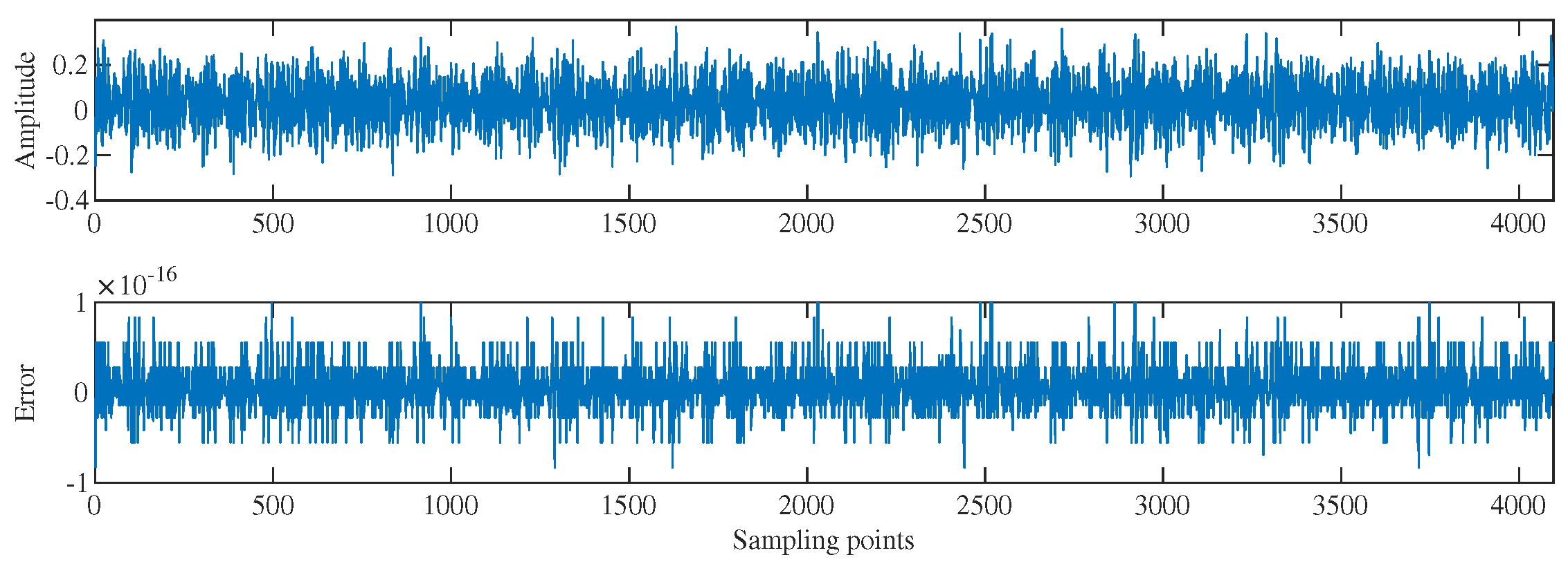
As illustrated in Figure 4, the one-level decomposition by LWT generates a total of six independent frequency components, and each component covers one sixth of the frequency information successively without redundancy and leakage because of the orthogonality, which is very effective and convenient for extracting the fault characteristic of the bearing from different frequency components. In this section, the reconstruction of the low-frequency and high-frequency components from Figure 4 using Equations (12) and (13) is illustrated in Figure 5. It can be observed that the reconstruction of this bearing fault data is highly accurate and free from Gibbs phenomena. The magnitude of the reconstruction error reaches , demonstrating the effectiveness and stability of the Legendre multiwavelet transform.

Figure 5.
Reconstruction and corresponding error of the bearing fault 1 by LWT.
3. The Proposed Method
This section primarily provides a detailed description of the usage steps for the proposed LW-BPNN method and elaborates on the description of the dataset mentioned earlier.
3.1. The Flowchart of the Proposed Method
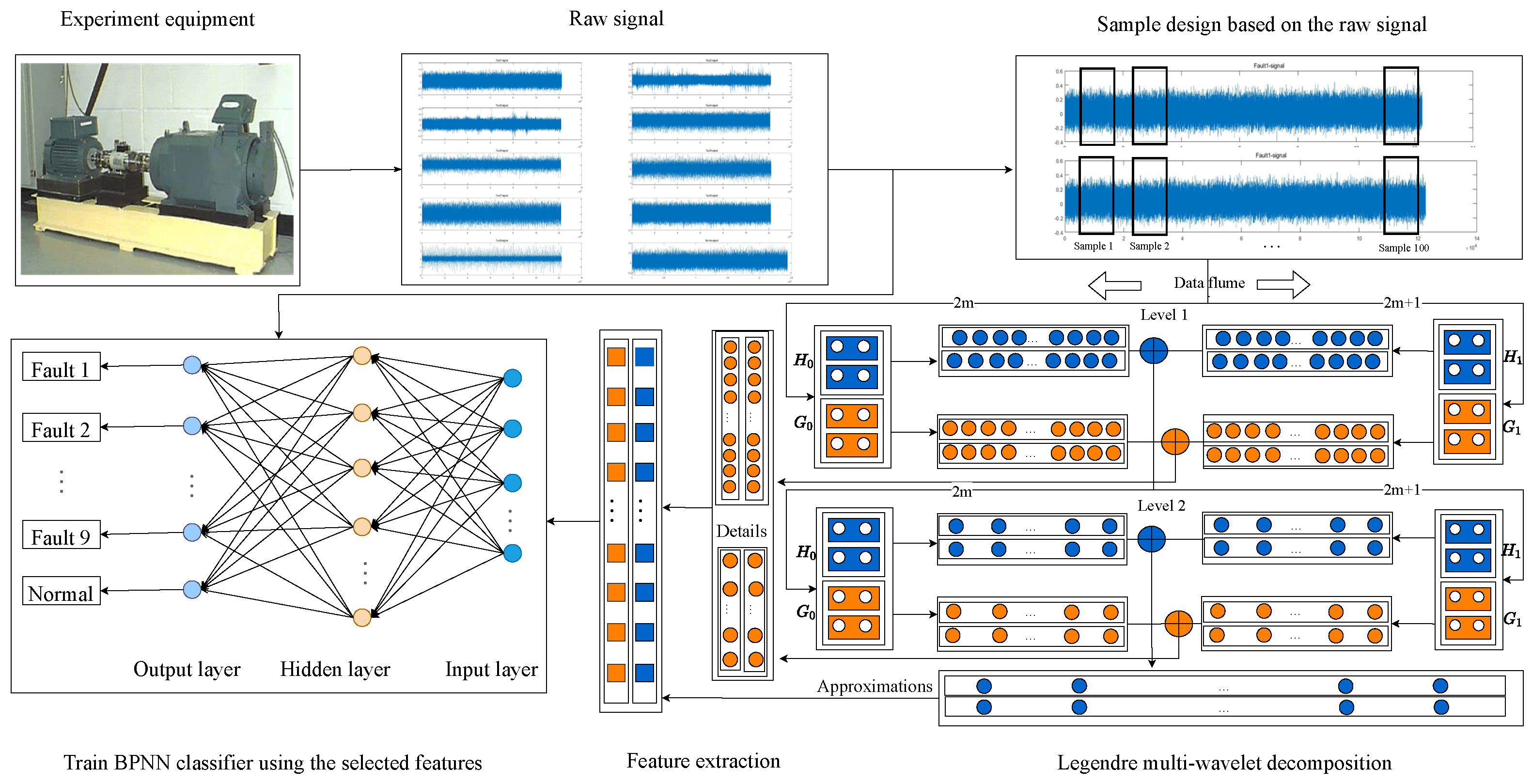
This subsection mainly describes the integration of LWD with the BPNN classifier for pattern classification in fault recognition and prognosis of the bearing. The following flowchart in Figure 6 elaborates on the fault diagnosis principle of the proposed method using Legendre multiwavelet bases with an order of

Figure 6.
Flowchart of the proposed approach for the bearing fault recognition.
Following the flowchart presented in Figure 6, the detailed steps of the proposed approach are outlined as follows:
Step 1: Collection of vibration signals from the bearing under different operational conditions encompassing ten fault types, utilizing the developed method for intelligent fault recognition.
Step 2: Firstly, select two Legendre scale base functions and their corresponding wavelet base functions. Secondly, preprocess the input vibration signal using a previously validated repeated oversampling approach for effective feature extraction. The processed signals are then sampled, resulting in 100 samples for each fault type and load. Eighty percent are designated as training samples while the remaining twenty percent serve as testing samples.
Step 3: Convolving the processed vibration signals using LWT at resolution level 2. This process generates approximation components and detail coefficients from the raw data, which are used to compute feature parameters such as RMS and SD. The resulting feature vector set is constructed using the computed RMS and SD values, serving as input for the classifier.
Step 4: Normalization of the fault feature vector set obtained from the two statistical parameters, RMS and SD, to a range between 0 and 1. The normalized training samples are used to train the BPNN classifier. Subsequently, the testing samples are input into the trained BPNN classifier to evaluate the bearing’s health condition.
Furthermore, to assess the effectiveness and stability of this method in extracting feature vectors from bearing fault data, an additional SVM classifier is implemented for recognizing various fault types. It’s worth noting that LWD functions as a multi-input and multi-output system, enhancing its capability to thoroughly extract complex signal characteristics more comprehensively and precisely compared to traditional wavelet methods.
3.2. Detailed Description of The Dataset
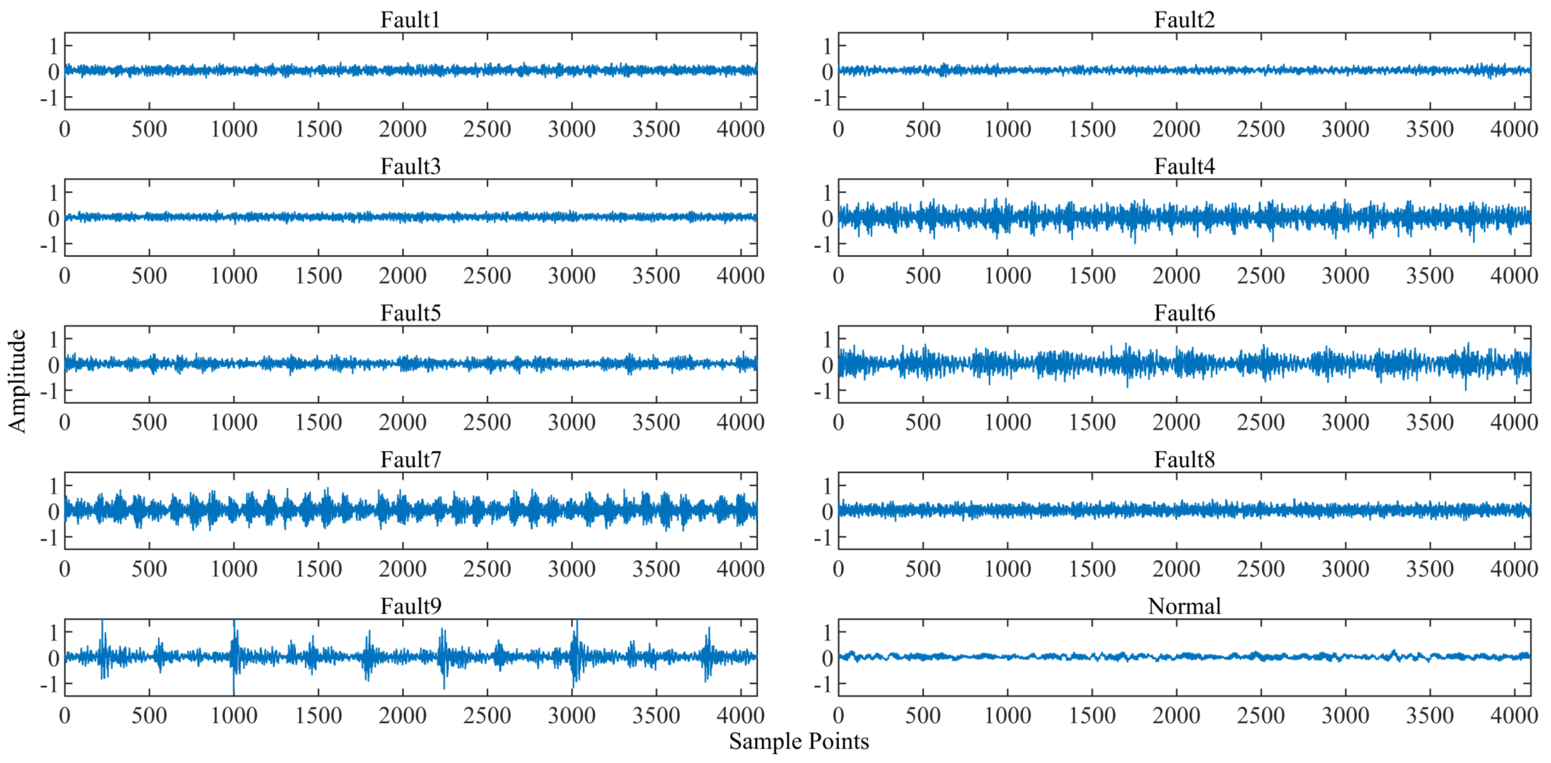
In this subsection, the dataset of the vibration signals of the bearing used in this paper is provided by the CWRU bearing dataset [33] and the corresponding ten fault categories are shown in Figure 7. Then, how to select the training samples and the testing samples of the fault condition recognition by using the vibration data of the bearing is specifically introduced.
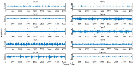
Figure 7.
The original vibration signal of 10 health conditions of the bearing.
The experimental setup utilized in the CWRU bearing dataset comprises a motor, a torque sensor, and a load motor. The test bearings at the drive end and fan end have model numbers 6205-2RS JEM and 6203-2RS JEM, respectively. These bearings exhibit four health conditions: ball fault, inner race fault, outer race fault, and normal condition, with damage sizes of 0.007, 0.014, and 0.021 inches, respectively. Each bearing undergoes testing at a constant speed (approximately 1730–1797 r/min) and operates under four different loads (0, 1, 2, and 3 hp). Table 2 provides a description of the operational conditions for the bearings.

Table 2.
Description of the operational conditions for the bearings.
From Table 2, it is evident that this dataset was collected at a constant speed range (1730–1797 rpm). Therefore, this paper selects the vibration data collected from the drive end bearing at a speed of 1797 rpm for analysis. Three different fault conditions along with the normal condition are chosen, labeled as: Outer Race Fault (OR), Inner Race Fault (IR), Ball Fault (B), and Normal, encompassing a total of 10 health states of the bearings, as detailed in Table 3, where category labels 1 through 9 correspond to fault 1 through 9.

Table 3.
Descriptions of the bearing health conditions.
In this paper, the raw data points under each health condition are evenly divided into 100 bearing samples. Each sample consists of 4096 data points obtained through a sliding window with partial overlap, resulting in a total of 1000 samples. Put differently, each original sample represents a vibration signal sequence of the bearing. The temporal waveforms of the raw data samples for 10 bearing health conditions are depicted in Figure 7.
4. Experimental Validation and Result Analysis
In this section, the proposed method is validated using the aforementioned dataset, and comparisons and analyses are conducted during the experiments. The dataset is employed to validate and assess the proposed method against comparative analyses. Additionally, all methods described in this paper were executed on a computer operating with Windows 11. The implementation of LWD and reconstruction was carried out using source code written in Matlab 2022a. The neural network implementation was based on Python 3.9, utilizing the PyTorch 1.10.0 deep learning framework. All models were trained on an Intel(R) Core(TM) i7-8565 U CPU and an NVIDIA RTX A4000 GPU.
4.1. Extraction Fault Characteristic
The extraction of valuable features from raw data is crucial for intelligent knowledge-based fault recognition methods. Poor feature extraction methods can result in bad diagnostic performance, even when employing potential classifiers. Therefore, the focus of this research lies in distinguishing and extracting the most valuable characteristic information with less reliance on expert experience and lower complexity compared to traditional methods.
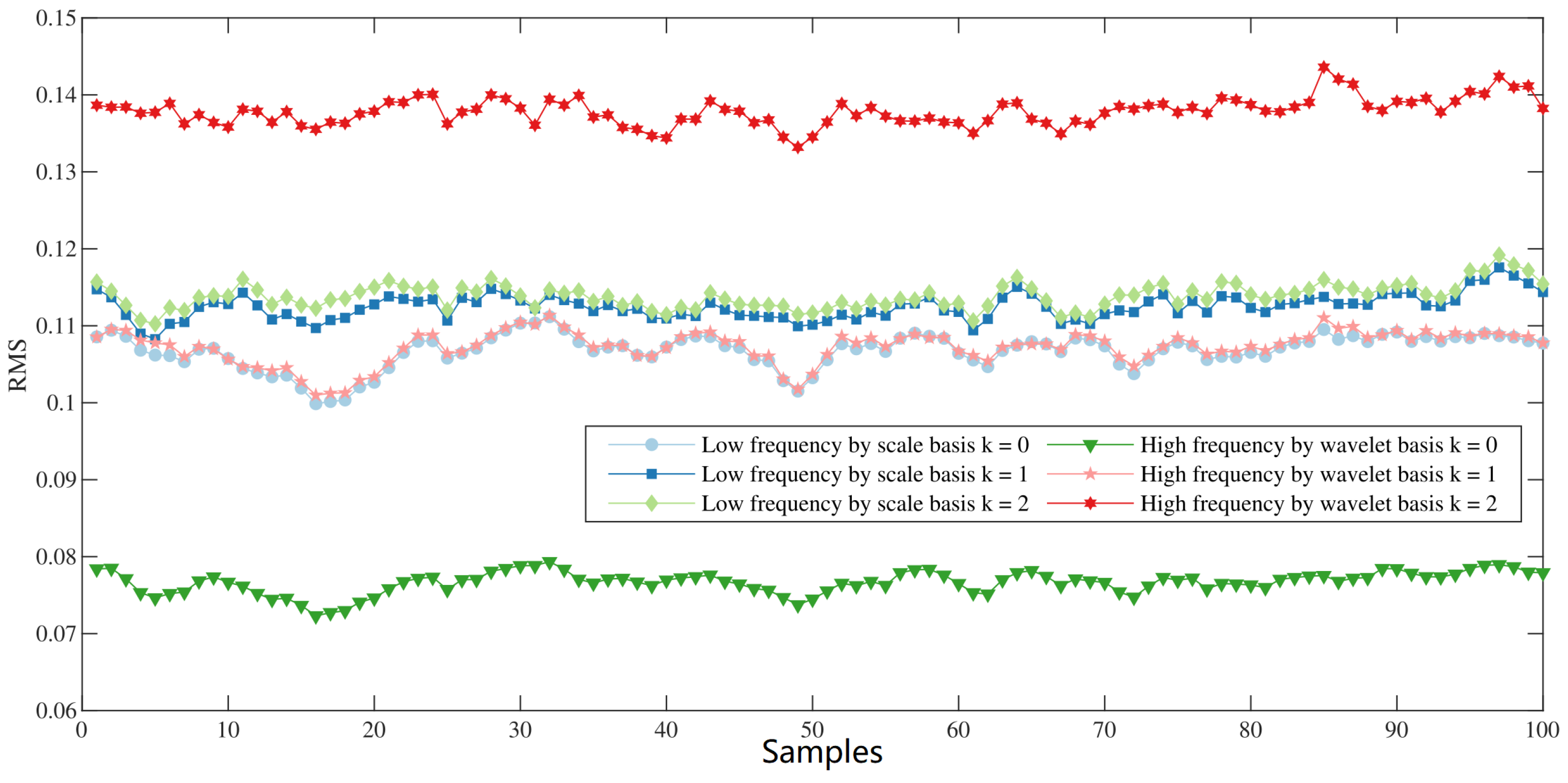
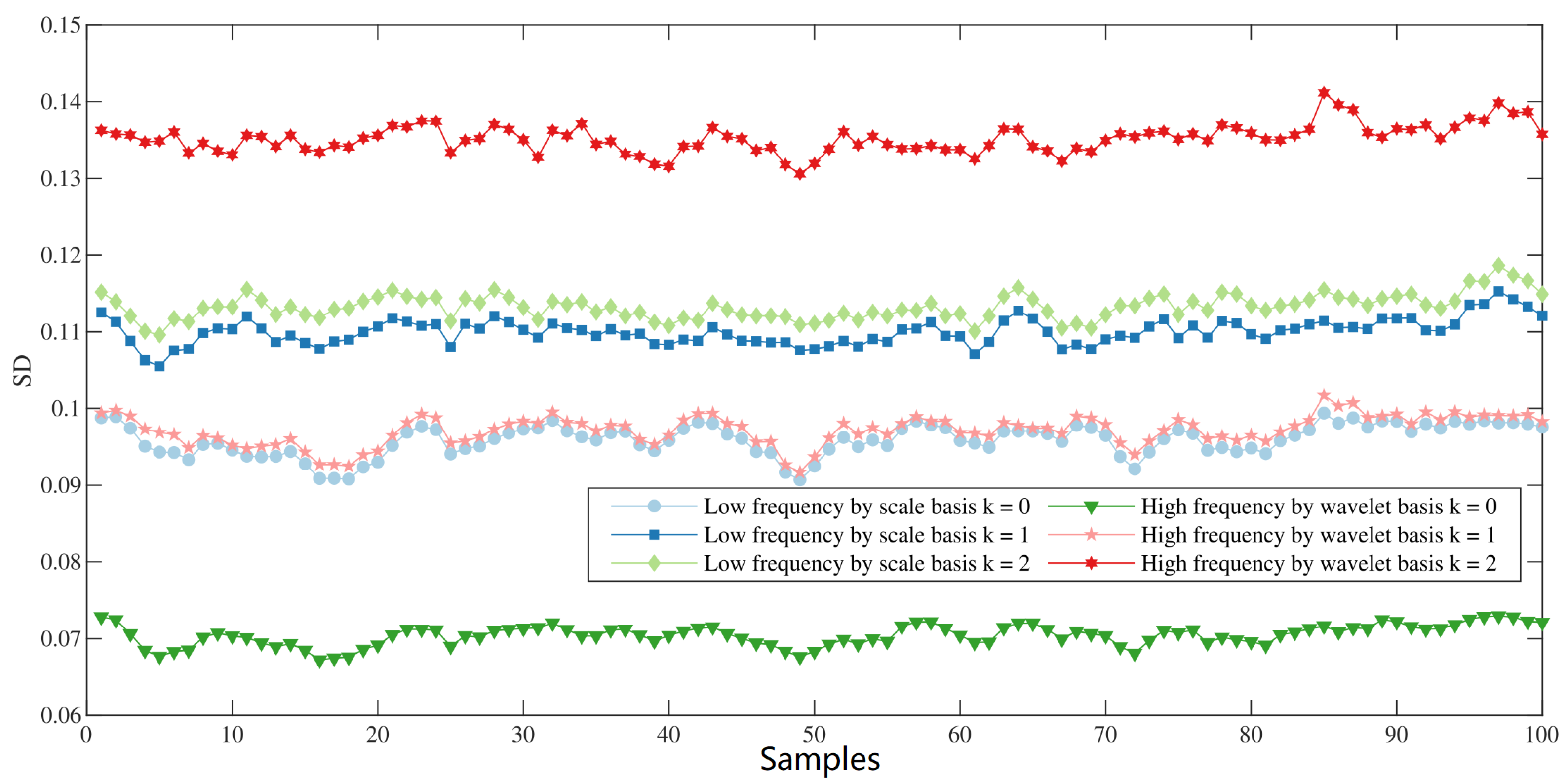
In this subsection, the distinguishing fault characteristics of LWD are thoroughly analyzed for scenarios involving individual fault types and all ten fault categories. The bearing fault data sample, consisting of 4096 points as mentioned in the previous subsection, is initially decomposed by LWD at resolution level with an order . The resultant low-frequency and high-frequency coefficient matrices are labeled as and , respectively. Utilizing Parseval’s theorem [32], RMS is employed as an extraction feature, retaining all pertinent information. Another selected feature is SD, effectively demonstrating the differences in frequency components and ideally suited for extracting features essential for fault detection and recognition. Then, the values of RMS and SD are computed using the aforementioned coefficient matrices as the feature vector set, comprising three low-frequency features and three high-frequency features, respectively. The variations corresponding to the number of samples obtained from a single fault type are detailed in Figure 8 and Figure 9 at different Legendre scales and Legendre wavelet bases, respectively.
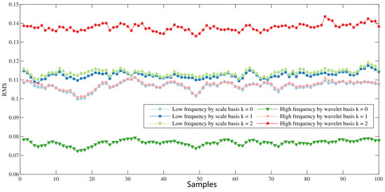
Figure 8.
The variation of RMS with the samples by different Legendre scale and wavelet bases.
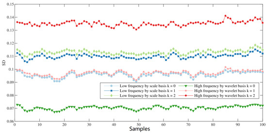
Figure 9.
The variation of SD with the samples by different Legendre scale and wavelet bases.
As illustrated in Figure 8 and Figure 9, six characteristic curves fluctuate rather than gather in one line, respectively, which demonstrate that the RMS and SD curves of different samples of a specific fault type have a number of differences in total. The results illustrate that LWD can powerfully represent and match the bearing comprehensive fault characteristic based on RMS and SD because of its orthogonality and various regularities. However, Figure 8 and Figure 9 show clear distinction between the low frequency and the high frequency , respectively. Legendre multiwavelet packet transform should be able to solve this issue in future work.
Furthermore, the distinguishing ability of LWD is also analyzed for different bearing fault types. Similarly, the variation of RMS and SD with the different health conditions of the bearing are shown at great length in Figure 10a,b.

Figure 10.
Variation of RMS (a) and SD (b) with different bearing fault types.
Correspondingly, it can be observed in Figure 10a,b that the differences of characteristic curves of ten bearing fault types are very obvious except for the low frequency and the high frequency , which illustrate that the extracted RMS and SD features can also automatically distinguish and learn the salient characteristic of different bearing fault types.
The primary advantage of extracting feature vectors using Legendre multiwavelets lies in their utilization of multiple scales and wavelet bases with orthogonality, allowing for the effective representation of the bearing’s prominent and comprehensive fault characteristics. Analyzing the distinguishing fault features’ capacity of LWD for recognizing bearing fault categories serves not only to verify the efficiency of RMS and SD feature vectors but also significantly reduces the complexity and reliance on expert knowledge compared to traditional feature extraction methods.
4.2. Comparison with Different Methods
In this section, the developed method in this work is first utilized to enhance the capacity of the bearing fault diagnosis, the corresponding effectiveness and stability are verified on different loads, and a better testing accuracy is achieved in comparison with the fault recognition methods based on Daubechies wavelet. Next, in contrast with the state-of-the-art intelligent fault diagnosis methods such as Fourier transform-CNN (FT-CNN) method, Fourier transform-RNN (FT-RNN) method and DW-BPNN method, the proposed LW-BPNN method achieves high average testing accuracy when adding different white noise, and the comparison results show that the proposed method is more robust and easier to implement. Finally, two-dimensional visualizations of different classification features using different fault diagnosis methods are elaborately described by the t-Distributed stochastic neighbor embedding (t-SNE) method, respectively.
4.2.1. Details of the Dataset Partition
The basic introduction to the bearing dataset for the intelligent fault recognition is described in Section 3.2. This subsection mainly illustrates how to divide the training samples and testing samples and process the dataset of the bearing with different fault patterns and different loads, respectively. For meeting the actual diagnostic requirements as much as possible, 800 samples of ten health conditions were randomly prepared for training and the remaining 200 samples were utilized to test the diagnostic performance of LW-BPNN approach, respectively. Additionally, the number of Legendre wavelet bases and resolution levels were chosen as three and four, respectively. The specific detailed description of the bearing data sample is shown below and listed in Table 4.

Table 4.
Four different load bearing data components.
Furthermore, in order to obtain the comparative results and rectify the effectiveness and the stability of the presented method, two classifiers, i.e., BPNN and SVM are adopted to diagnose the ten faults of the bearing (LW-BPNN method and LW-SVM method), respectively.
4.2.2. Experimental Results
In this subsection, the values of the statistical parameters RMS and SD are computed by using LWD coefficients at resolution level 4 and the corresponding results are utilized to devise the extraction of the significant feature vector for the classifiers, which are implemented to recognize the bearing fault categories under different loads, respectively. Of course, the average testing accuracy obtained is also utilized to compare with that of the DW method. The experimental results demonstrate that the proposed method achieves a better recognition accuracy and is very convenient to implement in real industrial applications and online diagnosis for rotating machinery.
In this experiment, the extracted feature, using only one feature parameter RMS, is a matrix with a size of , where 1000 is the number of the raw data samples for each load, is the dimension of the extraction feature vector, p is the number of Legendre wavelet bases, and n is the resolution level, respectively. According to the description in Table 4, the dimension of the feature vector is 15. Then, the training feature matrix with the size of for each load is inputted into the classifiers such as BPNN and SVM to classify the ten bearing fault types, and the testing data matrix is used to test the trained classifiers. Then, the process of another extracted feature SD is similar to this. In addition, in contrast with the method based on DWT, ’db2’ is selected in comparison with the proposed method since its order is same as that of Legendre wavelet base functions when . However, in real applications and in industry, machines and their bearings have to work under various types of load conditions. Therefore, the same training and testing samples must be conducted on the bearing dataset for the situation of all loads. Finally, all the average testing accuracies of the ten bearing faults are obtained by using only one feature parameter for extraction features are listed in Table 5 and Table 6 for comparison with each other, respectively.

Table 5.
Average testing accuracy by using RMS.

Table 6.
Average testing accuracy by using SD.
From Table 5, it can be observed that when using the RMS feature alone, the LW-SVM method performs consistently better than the DW-SVM method under single-load conditions. LW-SVM exhibits an improvement of 5.1%, 5.4%, 1.5%, and 0.1% over DW-SVM for 0 hp to 3 hp loads, resulting in an average diagnostic accuracy increase of 3.025%. This indicates the proposed approach significantly outperforms the DW-SVM method overall in this scenario. Similarly, Table 6 demonstrates that when utilizing the SD feature alone, the LW-SVM method consistently outperforms the DW-SVM method.
Similarly, the two feature parameters RMS and SD are also implemented to improve the recognition accuracy of the bearing, and the corresponding average testing accuracies achieved are demonstrated in detail in Table 7.

Table 7.
Average testing accuracy by using RMS and SD.
As shown in Table 7, in the testing samples, the lowest and highest fault diagnosis accuracies for individual loads are 86.8% and 98.8%, respectively, corresponding to the 2 hp load and 3 hp load. The diagnosis accuracies for all load conditions using both methods reach 100%. The experimental result of the developed method is also better than that of the DW method in total. Furthermore, by comparison with the recognition results in Table 5, Table 6 and Table 7, it can be clearly observed that the average testing accuracy slightly increases with the rise of the number of extracted features for each load. However, for the situation of all loads of the bearing, the highest accuracy rate of 100% is achieved for all four fault recognition methods described above with more training samples. Thus, it is possible to effectively improve the fault recognition accuracy by increasing the number of the training samples rather than adding more statistical parameters for the extraction features.
Additionally, the accuracy of each fault diagnosis was obtained by using the above two feature parameters is also described in Table 8 for each load of the bearing at the resolution level 4.

Table 8.
Diagnosis results of LW-BPNN methods using RMS and SD for each fault type.
As depicted in Table 8, distinct health conditions are clearly distinguished, except for BF14 and BF21 under the 0 hp load condition, as well as BF14 under the 1 hp and 2 hp load operations. This suggests the possibility that the type of ball fault might be more complex compared to inner and outer race faults. These experimental results demonstrate the proposed approach’s efficiency in diagnosing various fault categories of the bearing, showcasing high overall diagnostic accuracy.
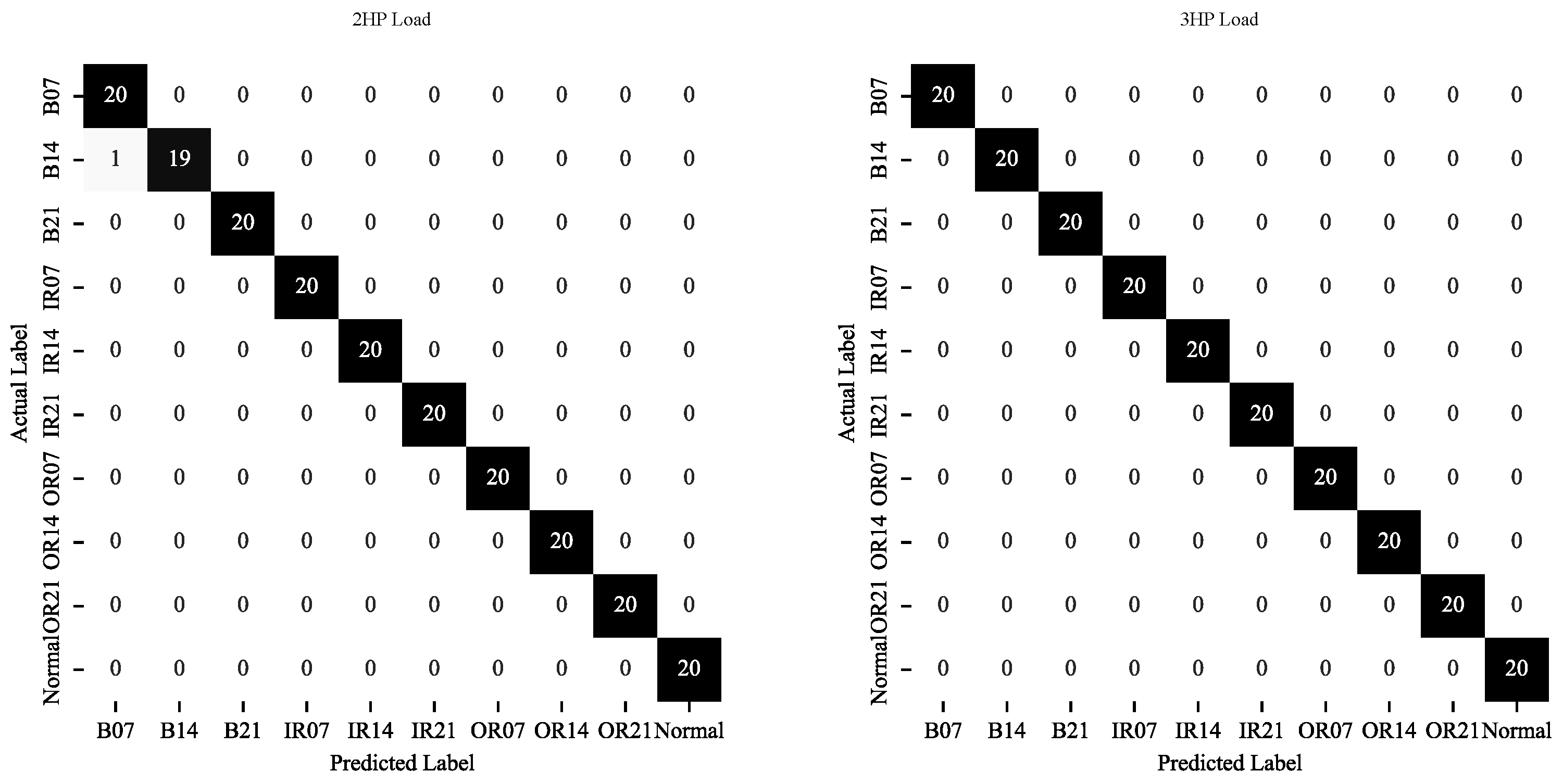
Furthermore, the multi-class confusion matrix provides a detailed reflection of the diagnosis results concerning different health conditions of the bearing, encompassing accuracy and error rates. Consequently, the detailed multi-class confusion matrices for the bearing data under 2 hp and 3 hp loads are illustrated in Figure 11, respectively.
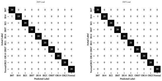
Figure 11.
Multi-class confusion matrices of the proposed approach for the 2 hp and 3 hp loads.
In Figure 11, the horizontal axis denotes the predicted label, and the ordinate axis represents actual label, respectively. As illustrated in Table 8 and Figure 11, the second health condition has the lowest accuracy rate of 95%, while the other nine health conditions can obtain the highest accuracy rate of 100% for the 2 hp load. The vast majority of the bearing fault patterns are rectified correctly for 2 hp and 3 hp loads in total. In fact, only 1 out of 200 testing samples were misclassified for the 2 hp load, which belongs to Class 2. Therefore, the proposed approach is able to rectify ten fault categories with high diagnosis precision under various working conditions.
Furthermore, for the purpose of avoiding particularity and contingency, the experiment was conducted over 10 trials. The comparison recognition results of the four methods mentioned above are shown at length in Figure 12 for the situation of the 3 hp load of the bearing data.

Figure 12.
Diagnosis accuracy of the four methods for 10 trials.
The detailed recognition results in each trial are shown in Figure 12, where the average testing accuracies obtained by the four methods are described in Table 7 as 98.90%, 99.80%, 98.80%, and 100% for the 10 trials, respectively, demonstrating more stability and better recognition accuracy of the proposed method in comparison with DW methods. It should be emphasized that the accuracy rate obtained by SVM classifier is lower than that of BPNN classifier. If the dimension of the extracted features is increased, the diagnosis accuracy and the stability by the SVM classifier can be slightly improved.
It is worth noting that BPNN and SVM classifiers are applied to fault classification in these approaches, respectively. For the BPNN classifier, the number of hidden nodes is 24, the largest training number is 2000, the learning rate used in this work is 0.25, and the training error is 0.001, respectively. In the standard SVM, the penalty factor and the order of polynomial kernel are 1 and 3, respectively. Additionally, the configuration parameters of the 10 trials are elaborately described in Table 9.

Table 9.
The parameters of the four methods for 10 trials.
As demonstrated in Figure 12 and Table 9, the developed method with lower dimension feature vector and simpler network structure can effectively accomplish the intelligent fault diagnosis of the bearing, and highest recognition accuracy and more stability by using only two feature parameters are obtained to a great extent, representing a benefit for real industrial applications.
4.3. Comparison of Different Methods under Noisy Background Conditions
In this subsection, in order to rectify the powerful ability to distinguish and extract the salient and comprehensive bearing fault characteristics of the proposed method, several other popular data-driven methods such as FT-CNN method, FT-RNN method, DW-SVM method, and DW-BPNN method were applied to compare with each other. Moreover, owing to the harsh working conditions of the bearing, vibration signals are often interfered with by noise, which further increases the difficulty of characteristics extraction and fault diagnosis. Therefore, the influence of noise on the effectiveness and robustness of these methods was analyzed by using the signal-to-noise ratios (SNRs) method by adding white noise.
In this experiment, the LW-BPNN method developed in this work with signal-to-noise ratios of 4 dB, 2 dB, 0 dB, −2 dB, −4 dB, −6 dB, −8 dB, −10 dB, −12dB was implemented to diagnose the health conditions of the bearing for the 3 hp load of the bearing data. The corresponding signal-to-noise ratios are obtained from the ratio between the original signal power and the noise power, respectively. Specifically, the same noise is added to the training set and the testing set to identify the resistance noise ability of the proposed method by using only two feature parameters RMS and SD. Table 10 elaborately describes the testing results of the different fault recognition methods.

Table 10.
Diagnostic accuracy of different methods under a series of noise backgrounds.
Table 10 clearly demonstrates the testing results across different SNRs, indicating that the LW-BPNN method achieves the highest testing accuracy and exhibits effective resistance to noise. It shows a slight decrease in accuracy when compared to scenarios without added noise, and it is overall less affected by low SNRs as low as −6 dB in comparison to other methods. Notably, this method maintains a high recognition rate of over 99% at high SNRs, specifically −4 dB. Even at the lowest SNR of −12 dB, the proposed method maintains the highest recognition accuracy at 94.80%. These testing results suggest that deep learning methods often struggle in low SNR situations due to their inadequate noise resistance. Conversely, the proposed approach demonstrates superior robustness against noise, making it more suitable for bearing fault recognition in low-noise environments, leveraging the powerful denoising ability of the wavelet method. Additionally, optimizing the SVM classifier with an appropriate method will be necessary to enhance its stability and robustness in future applications.
Furthermore, the corresponding experimental configuration parameters involved in these methods are listed in detail as follows.
Classifiers: The input classifiers consist of thirty dimensions derived from two feature parameters, RMS and SD. These parameters are calculated on the low- and high-frequency components at resolution level and order of Legendre wavelet base functions, respectively. For the BPNN classifier, a single hidden layer comprising 24 neurons utilizing the sigmoidal function and a softmax classifier are employed to validate bearing diagnosis for comparison. The learning rate is set at 0.001, with a maximum of 2000 iterations; iteration stops when the loss falls below 0.001. The output layer entails classification labels ranging from 1 to 10, consistent with other methods for comparison. For the SVM classifier, the selected parameters include a penalty factor of 1 and a polynomial kernel order of 3.
FT-CNN method: The raw data is transformed by Fourier transform. Then, the frequency components obtained are fed into 1D-CNN for extraction fault features. There are three convolutional layers and three corresponding pooling layers in 1D-CNN, and the convolutional layers contain 32, 64, and 64 kernels and the filter length is 3 for every kernel, respectively. Finally, a fully-connected layer and a softmax classifier are attached on the top.
FT-RNN method: Similar to FT-CNN method, the raw data is transformed by Fourier transform. Then, the frequency components obtained are fed into RNN for extraction fault features. There is a hidden layer of RNN and the size of the hidden layer is 128.
DW method: Db 2 is adopted to process the raw bearing data for comparison because the order is same as that of Legendre multiwavelet with three wavelet bases. The configuration parameters of the two classifiers are the same as that mentioned in Table 9.
LW method: Legendre multiwavelet with three scale bases and corresponding three wavelet base functions is adopted to decompose the raw bearing data at the resolution level 4. Additionally, the parameters of the two classifiers applied to verify the bearing faults are the same as DW methods except for the thirty-dimensional input for the classifiers.
Then, the bearing fault classification results of these methods with addition of −2 dB noise for the 10 trials conducted to avoid contingency are illustrated at great length in Figure 13.

Figure 13.
Diagnosis accuracy of the above methods with addition of −2 dB noise for 10 trials.
As depicted in Figure 13, the LW-BPNN method demonstrates superior performance when subjected to −2 dB noise, surpassing all methods except the DW-BPNN approach. Additionally, both LW and DW methods achieve higher testing accuracy rates compared to FT-CNN and FT-RNN methods across all noise environments. The experiments illustrate that the LW method effectively identifies various fault categories in bearings and exhibits better stability and robustness compared to other methods in diverse noise environments. To illustrate the impact of noise on diagnostic results, Figure 14 presents the multi-class confusion matrices of FT-CNN and LW-BPNN under the scenario of adding −2 dB noise.
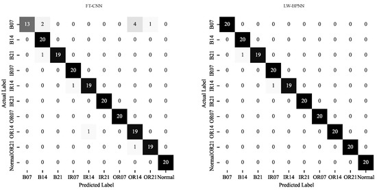
Figure 14.
Multi-class confusion matrices of FT-CNN and the proposed method with the addition of −2 dB noise.
The results in Figure 14 confirm the effectiveness and robustness of applying FT-CNN and LW-BPNN methods in bearing fault diagnosis under high-noise conditions. In fact, under the 3 hp load scenario, the FT-CNN and LW-BPNN methods misclassified 11 and 2 out of 200 testing samples, respectively. Additionally, for higher signal-to-noise ratios, the Daubechies wavelet denoising method was applied to classify the health status of denoised fault data using FT-CNN and LW-BPNN methods. Figure 15 demonstrates the detailed diagnostic accuracy achieved using the denoising method under −2 dB noise.

Figure 15.
Multi-class confusion matrices obtained by denoising method.
It can be clearly seen from Figure 15 that the FT-CNN method and the proposed method combining the Daubechies wavelet denoising method are very effective and robust for bearing fault diagnosis under a high signal-to-noise ratio. It is noted that the diagnostic accuracy is improved by the DW denoising method. The vast majority of the bearing fault types are distinguished correctly for 3 hp load in total. In fact, 4 and 1 out of 200 testing samples are misclassified by these two methods for the 3 hp load, respectively. Consequently, the proposed integrated DW denoising method is powerful and robust to identify ten fault categories with high diagnosis precision under a low signal-to-noise ratio environment.
4.4. Visualizing The Features
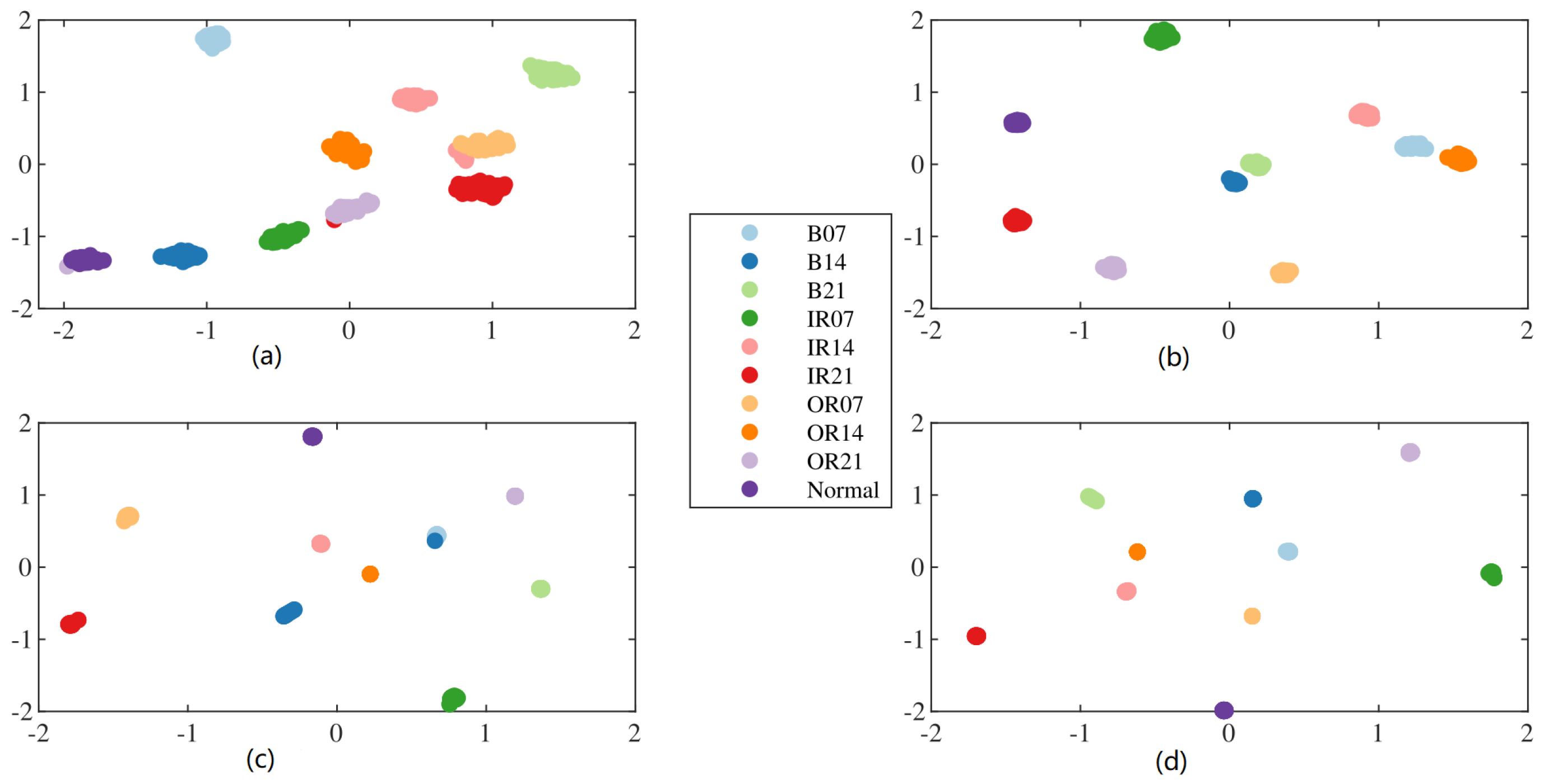
In this subsection, the t-SNE method is also applied to visualize the learned features in the two-dimensional space for different fault diagnosis methods mentioned in the above subsection without any noise. Figure 16a shows the clustering results obtained by FT-CNN method, and the other clustering maps based on the features learned by FT-RNN method, DW-BPNN method and the proposed LW-BPNN method are shown in detail in Figure 16b–d, respectively.
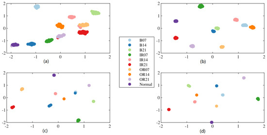
Figure 16.
Features visualization based on t-SNE: (a) FT-CNN method, (b) FT-RNN method, (c) DW-BPNN method, (d) the proposed method.
From the visualized results of Figure 16a–d, it is demonstrated that the proposed approach has been more effective and stable in distinguishing between the characteristics of each fault of the bearing when compared to other methods. As demonstrated in Figure 16a, the fault features extracted by FT-CNN from data samples of the ten health conditions achieve the least clustering effect on bearing faults. There are still several samples overlapped between the inner race fault and the outer race fault. As shown in Figure 16b,c, the features learned by the FT-RNN method have a good clustering result for the bearing’s inner race fault and the outer race fault, but in Figure 16c there is a slight overlap between the ball fault patterns. As shown in Figure 16d, the proposed method almost achieves effective separation of the ten fault types, and the distribution of the extracted features for each fault pattern is more concentrated. Therefore, the extracted features of the same health condition by using the proposed method are best clustered and the extracted features of different health conditions are separated accurately.
5. Conclusions
An effective and reliable intelligent fault recognition method for bearings is developed in this paper. The proposed method utilizes Legendre scale and wavelet bases with rich properties, in particular, orthogonality and various alternative regularities. Feature parameter extraction in the proposed method is achieved through multiple Legendre scales and wavelet bases, eliminating reliance on expert knowledge. By coupling this approach with the BPNN classifier, it achieves the highest diagnostic accuracy and computational efficiency. For comparisons, popular fault recognition methods such as FT-CNN method, FT-RNN method, DW-BPNN method and DW-SVM methods were also conducted on the same bearing dataset with the addition of different ratios of white noise. The experimental results illustrate that the proposed method achieves the highest diagnostic accuracy, with 100% and over 99% under the conditions of no additional noise and addition of −4 dB noise, respectively, and shows more robustness and feasibility than other methods applied to identify the health conditions of bearings. In future work, LWD should be combined with a deep neural network to identify rotating machinery faults with highly non-stationary, weak, and compound fault signals.
Author Contributions
Conceptualization, Z.F.; Methodology, X.Z.; Software, Z.F. and Z.L.; Validation, X.Z. and L.C.; Formal analysis, X.Z., Z.F. and Z.L.; Investigation, L.C.; Resources, Z.L.; Data curation, L.C.; Writing—original draft, X.Z. and Z.F. All authors have read and agreed to the published version of the manuscript.
Funding
This research was funded by Chongqing CSTC of China, grant number cstc2019jcyj-msxmX0386 and cstc2020jcyj-msxmX0232.
Data Availability Statement
Data are contained within the article.
Acknowledgments
The authors are extremely grateful to the editor and referees for their valuable comments that greatly improved the quality of this paper.
Conflicts of Interest
The authors declare no conflict of interest.
Abbreviations
The following abbreviations are used in this manuscript:
| LW-BPNN | Legendre multiwavelet transform combined with BPNN |
| BPNN | Back propagation neural network |
| RMS | Root mean square |
| SD | Standard deviation |
| SVM | Support vector machine |
| CNN | Convolutional neural network |
| RNN | Recurrent neural network |
| LWT | Legendre multiwavelet transform |
| LWD | Legendre multiwavelet decomposition |
| CWRU | Case Western Reserve University bearing dataset |
| FT-CNN | Fourier transform combined with CNN |
| FT-RNN | Fourier transform combined with RNN |
| DW-BPNN | Daubechies wavelet combined with BPNN |
| DW-SVM | Daubechies wavelet combined with SVM |
| LW-SVM | Legendre multiwavelet transform combined with SVM |
| t-SNE | t-Distributed stochastic neighbor embedding |
| SNRs | Signal-to-noise ratios |
References
- Randall, R.B.; Antoni, J. Rolling element bearing diagnostics—A tutorial. Mech. Syst. Signal Process. 2011, 25, 485–520. [Google Scholar] [CrossRef]
- Yang, S.; Gu, X.; Liu, Y.; Hao, R.; Li, S. A general multi-objective optimized wavelet filter and its applications in fault diagnosis of wheelset bearings. Mech. Syst. Signal Process. 2020, 145, 106914. [Google Scholar] [CrossRef]
- Dong, X.; Li, G.; Jia, Y.; Xu, K. Multiscale feature extraction from the perspective of graph for hob fault diagnosis using spectral graph wavelet transform combined with improved random forest. Measurement 2021, 176, 109178. [Google Scholar] [CrossRef]
- Rai, A.; Upadhyay, S. A review on signal processing techniques utilized in the fault diagnosis of rolling element bearings. Tribol. Int. 2016, 96, 289–306. [Google Scholar] [CrossRef]
- Wei, H.; Zhang, Q.; Shang, M.; Gu, Y. Extreme learning Machine-based classifier for fault diagnosis of rotating Machinery using a residual network and continuous wavelet transform. Measurement 2021, 183, 109864. [Google Scholar] [CrossRef]
- Chen, J.; Li, Z.; Pan, J.; Chen, G.; Zi, Y.; Yuan, J.; Chen, B.; He, Z. Wavelet transform based on inner product in fault diagnosis of rotating machinery: A review. Mech. Syst. Signal Process. 2016, 70–71, 1–35. [Google Scholar] [CrossRef]
- Almounajjed, A.; Sahoo, A.K.; Kumar, M.K. Diagnosis of stator fault severity in induction motor based on discrete wavelet analysis. Measurement 2021, 182, 109780. [Google Scholar] [CrossRef]
- Haidong, S.; Junsheng, C.; Hongkai, J.; Yu, Y.; Zhantao, W. Enhanced deep gated recurrent unit and complex wavelet packet energy moment entropy for early fault prognosis of bearing. Knowl.-Based Syst. 2020, 188, 105022. [Google Scholar] [CrossRef]
- Li, X.; Jiang, H.; Wang, R.; Niu, M. Rolling bearing fault diagnosis using optimal ensemble deep transfer network. Knowl.-Based Syst. 2021, 213, 106695. [Google Scholar] [CrossRef]
- Yan, X.; She, D.; Xu, Y.; Jia, M. Deep regularized variational autoencoder for intelligent fault diagnosis of rotor–bearing system within entire life-cycle process. Knowl.-Based Syst. 2021, 226, 107142. [Google Scholar] [CrossRef]
- Shao, H.; Jiang, H.; Wang, F.; Zhao, H. An enhancement deep feature fusion method for rotating machinery fault diagnosis. Knowl.-Based Syst. 2017, 119, 200–220. [Google Scholar] [CrossRef]
- Cheng, Y.; Wang, Z.; Chen, B.; Zhang, W.; Huang, G. An improved complementary ensemble empirical mode decomposition with adaptive noise and its application to rolling element bearing fault diagnosis. ISA Trans. 2019, 91, 218–234. [Google Scholar] [CrossRef]
- Yuan, R.; Lv, Y.; Li, H.; Song, G. Robust Fault Diagnosis of Rolling Bearings Using Multivariate Intrinsic Multiscale Entropy Analysis and Neural Network Under Varying Operating Conditions. IEEE Access 2019, 7, 130804–130819. [Google Scholar] [CrossRef]
- Yan, X.; Jia, M. Intelligent fault diagnosis of rotating machinery using improved multiscale dispersion entropy and mRMR feature selection. Knowl. Based Syst. 2019, 163, 450–471. [Google Scholar] [CrossRef]
- Dou, D.; Yang, J.; Liu, J.; Zhao, Y. A rule-based intelligent method for fault diagnosis of rotating machinery. Knowl. Based Syst. 2012, 36, 1–8. [Google Scholar] [CrossRef]
- Asr, M.Y.; Ettefagh, M.M.; Hassannejad, R.; Razavi, S.N. Diagnosis of combined faults in Rotary Machinery by Non-Naive Bayesian approach. Mech. Syst. Signal Process. 2017, 85, 56–70. [Google Scholar] [CrossRef]
- Wang, X.; Zi, Y.; He, Z. Multiwavelet construction via an adaptive symmetric lifting scheme and its applications for rotating machinery fault diagnosis. Meas. Sci. Technol. 2009, 20, 045103. [Google Scholar] [CrossRef]
- Yan, R.; Gao, R.X.; Chen, X. Wavelets for fault diagnosis of rotary machines: A review with applications. Signal Process. 2014, 96, 1–15. [Google Scholar] [CrossRef]
- Jiang, G.; He, H.; Yan, J.; Xie, P. Multiscale Convolutional Neural Networks for Fault Diagnosis of Wind Turbine Gearbox. IEEE Trans. Ind. Electron. 2019, 66, 3196–3207. [Google Scholar] [CrossRef]
- Zheng, X.; Yang, X.; Su, H.; Qiu, L. Discontinuous Legendre wavelet element method for elliptic partial differential equations. Appl. Math. Comput. 2011, 218, 3002–3018. [Google Scholar] [CrossRef]
- Huang, H.; Li, K.; Su, W.; Bai, J.; Xue, Z.; Zhou, L.; Su, L.; Pecht, M. An improved empirical wavelet transform method for rolling bearing fault diagnosis. Sci. China Technol. Sci. 2020, 63, 2231–2240. [Google Scholar] [CrossRef]
- Kuncan, M.; Kaplan, K.; Mi?naz, M.R.; Kaya, Y.; Ertunç, H.M. A novel feature extraction method for bearing fault classification with one dimensional ternary patterns. ISA Trans. 2020, 100, 346–357. [Google Scholar] [CrossRef]
- Liu, H.; Zhou, J.; Zheng, Y.; Jiang, W.; Zhang, Y. Fault diagnosis of rolling bearings with recurrent neural network-based autoencoders. ISA Trans. 2018, 77, 167–178. [Google Scholar] [CrossRef]
- Pandya, D.; Upadhyay, S.; Harsha, S. Fault diagnosis of rolling element bearing with intrinsic mode function of acoustic emission data using APF-KNN. Expert Syst. Appl. 2013, 40, 4137–4145. [Google Scholar] [CrossRef]
- Shao, H.; Jiang, H.; Zhao, H.; Wang, F. A novel deep autoencoder feature learning method for rotating machinery fault diagnosis. Mech. Syst. Signal Process. 2017, 95, 187–204. [Google Scholar] [CrossRef]
- Shang, C.; Yang, F.; Huang, D.; Lyu, W. Data-driven soft sensor development based on deep learning technique. J. Process Control 2014, 24, 223–233. [Google Scholar] [CrossRef]
- Shi, J.; Peng, D.; Peng, Z.; Zhang, Z.; Goebel, K.; Wu, D. Planetary gearbox fault diagnosis using bidirectional-convolutional LSTM networks. Mech. Syst. Signal Process. 2022, 162, 107996. [Google Scholar] [CrossRef]
- Meng, L.; Xiang, J.; Wang, Y.; Jiang, Y.; Gao, H. A hybrid fault diagnosis method using morphological filter–translation invariant wavelet and improved ensemble empirical mode decomposition. Mech. Syst. Signal Process. 2015, 50–51, 101–115. [Google Scholar] [CrossRef]
- Manjurul Islam, M.; Kim, J.M. Reliable multiple combined fault diagnosis of bearings using heterogeneous feature models and multiclass support vector Machines. Reliab. Eng. Syst. Saf. 2019, 184, 55–66. [Google Scholar] [CrossRef]
- Li, J.; Yao, X.; Wang, X.; Yu, Q.; Zhang, Y. Multiscale local features learning based on BP neural network for rolling bearing intelligent fault diagnosis. Measurement 2020, 153, 107419. [Google Scholar] [CrossRef]
- Yan, X.; Liu, Y.; Jia, M. Multiscale cascading deep belief network for fault identification of rotating machinery under various working conditions. Knowl. Based Syst. 2020, 193, 105484. [Google Scholar] [CrossRef]
- Alpert, B.K. A Class of Bases in L2 for the Sparse Representation of Integral Operators. SIAM J. Math. Anal. 1993, 24, 246–262. [Google Scholar] [CrossRef]
- Case Western Reserve University Bearing Fault Dataset; Case School of Engineering: Cleveland, OH, USA, 2012.
Disclaimer/Publisher’s Note: The statements, opinions and data contained in all publications are solely those of the individual author(s) and contributor(s) and not of MDPI and/or the editor(s). MDPI and/or the editor(s) disclaim responsibility for any injury to people or property resulting from any ideas, methods, instructions or products referred to in the content. |
© 2023 by the authors. Licensee MDPI, Basel, Switzerland. This article is an open access article distributed under the terms and conditions of the Creative Commons Attribution (CC BY) license (https://creativecommons.org/licenses/by/4.0/).


