Multi-Sensor Data Fusion for Real-Time Multi-Object Tracking

Abstract

Sensor data fusion is essential for environmental perception within smart traffic applications. By using multiple sensors cooperatively, the accuracy and probability of the perception are increased, which is crucial for critical traffic scenarios or under bad weather conditions. In this paper, a modular real-time capable multi-sensor fusion framework is presented and tested to fuse data on the object list level from distributed automotive sensors (cameras, radar, and LiDAR). The modular multi-sensor fusion architecture receives an object list (untracked objects) from each sensor. The fusion framework combines classical data fusion algorithms, as it contains a coordinate transformation module, an object association module (Hungarian algorithm), an object tracking module (unscented Kalman filter), and a movement compensation module. Due to the modular design, the fusion framework is adaptable and does not rely on the number of sensors or their types. Moreover, the method continues to operate because of this adaptable design in case of an individual sensor failure. This is an essential feature for safety-critical applications. The architecture targets environmental perception in challenging time-critical applications. The developed fusion framework is tested using simulation and public domain experimental data. Using the developed framework, sensor fusion is obtained well below 10 milliseconds of computing time using an AMD Ryzen 7 5800H mobile processor and the Python programming language. Furthermore, the object-level multi-sensor approach enables the detection of changes in the extrinsic calibration of the sensors and potential sensor failures. A concept was developed to use the multi-sensor framework to identify sensor malfunctions. This feature will become extremely important in ensuring the functional safety of the sensors for autonomous driving.

1. Introduction

Autonomous or self-driving vehicles are currently an important research field to which many companies and research centers are actively contributing. Environmental perception, namely the detection of all traffic users and interpretation of the traffic situations, is a key factor to enabling a vehicle to drive autonomously (i.e., to perform path-planning based on the environmental perception and drive a safe trajectory within the given situation from one place to another). Therefore, researchers and car manufacturers use multiple sensors in autonomous vehicles to detect and classify all traffic users with high probability and accurate positions. In many driving situations, a single camera is already sufficient for environmental perception. However, under bad weather conditions or in complex traffic situations, the appropriate approach is to use different physical sensors (heterogeneous sensors) in the vehicles (e.g., radar, LiDAR, and cameras) which cover the same field of view for cooperative perception to reduce the probability of detection errors.

A traffic situation is described using an object state vector for each detected road user. These state vectors contain attributes related to the objects (e.g., type of road user (truck, car, bicyclist, pedestrian, etc.), location, orientation, size, and speed). Human drivers mainly use their eyes to detect objects and generate their object states. Therefore, some car manufacturers develop their environmental perception solely based on cameras, but others are also utilizing additional sensors [1]. Specifically, accurate distance measurement is still challenging using mono cameras, even though machine learning (ML)-based depth estimation is progressing. Nevertheless, using additional sensors such as radar and LiDAR, where each sensor type provides new information due to the different sensing principles, will improve the accuracy of computer vision-based object detection and localization. For safe driving, the state vectors need to provide the highest degree of reliability and require a good overlap of information from different sensors. However, observing the same object with multiple sensors and generating multiple object states does not provide many advantages unless the data are fused to generate one consolidated object state.

Fusion approaches in environmental perception are generally divided according to the abstraction level where fusion is performed, namely low-level fusion (LLF), middle-level fusion (MLF), and high-level fusion (HLF) [2]. Fusion algorithms can be further categorized into two main categories based on the approach: (1) traditional fusion methods which use state estimators such as Kalman filters and (2) machine learning-based methods such as deep neural networks. In the LLF approach, fusion algorithms receive sensor data with no or minimal preprocessing (hardware-level process) [2]. It is a beneficial approach for machine learning methods, where preserving all information potentially increases the object detection accuracy [3]. Although LLF is characterized by a low false-positive rate with respect to object detection, it makes the data fusion process complex and requires higher hardware performance. In the MLF approach, a feature extraction algorithm is applied in the first step to the raw data, and the fusion algorithm receives features from the respective sensors. Therefore, it is also called feature-level fusion [4]. Finally, in the HLF approach, the fusion algorithm receives an object list or a tracked object list from the sensors. Therefore, sensors can easily be added to or removed from the fusion algorithm, which makes HLF scalable. However, less information for detection and classification is passed to the sensor fusion process because the sensor’s raw data are already processed by each sensor independently to estimate objects. The main advantage of high-level fusion is that it requires less computational power compared with LLF and MLF. Furthermore, minimal data are communicated when multiple computing units at the sensor level are used [5]. Since processing is performed at the sensor level, all sensor-relevant details are kept at the sensor level, allowing the fusion module to process the data in an abstract manner [6] (e.g., data privacy conforms because no images, but only abstract object lists, are communicated).

In this paper, a modular fusion framework for environmental perception is presented which is based on HLF (i.e., it takes the object lists from the individual sensors as input). The framework consists of several modules. First, the object lists are transformed into the coordinate system of the vehicle. Secondly, object association is performed based on the Hungarian algorithm. Afterward, fusion and tracking are performed by employing an unscented Kalman filter followed by a movement compensation module. The advantages of the framework are the following:

• The sensor fusion framework has large flexibility regarding the types and number of sensors.
• The framework reacts robustly in case of individual sensor failures.
• The framework is real-time capable.
• The fusion framework is generic, and thus it can be also used for static sensor applications such as roadside units (RSU). In this case, the movement compensation module is removed (i.e., the velocity is set to zero).

The benefits of the fusion framework are evaluated in a simulation environment and with public domain data. To achieve validation through simulation, different sensor models for the camera, radar, and LiDAR are used. In this paper, it is demonstrated that the sensor fusion framework provides a good estimation of the object state in a time-efficient manner.

In Section 2, the state of the art and the work related to the presented fusion framework are summarized. Section 3 details the framework with modules such as coordinate transformation, object association, unscented Kalman filters, and movement compensation for sensor fusion. In Section 4, the object lists which are provided by the different sensors are discussed, and the simulation tool used as the ground truth is introduced. In Section 5, the fusion results are presented for different simulation and experimental scenarios. In Section 6, the benefits of using object list-based fusion in sensor fault detection are discussed. Section 7 concludes this paper with a summary and an outlook on future work.

2. Related Work

Sensor data fusion is used in many fields (robotics, diagnostics in medicine, Industry 4.0, smart home systems, etc.) [7]. All three fusion methods mentioned in the introduction section have well-known advantages and disadvantages [8]. For example, LLF does not require a sensor-to-sensor object association method because the raw sensor data are unified (e.g., two or more sensor data are merged before an object is detected or classified). However, since the data from different sensors need to be unified before object detection, LLF requires accurate time synchronization between the sensors (i.e., the sensor signals are taken at the same time and also consume more computational resources). In addition, when the sensor data need to be transferred, this requires high bandwidth. In contrast, HLF requires minimal bandwidth, and time synchronization between sensors is rather uncritical. However, since object detection occurs at the sensor level, an additional object association is required. Furthermore, LLF claims to be statistically more accurate than HLF in terms of object detection and classification. This is because if an object is detected with a low probability by the detection algorithm in HLF, this detection can be neglected for further processes, since all sensors perform the detection independently from each other. However, in the case of LLF, the sensor data are unified before object detection, and therefore, multiple pieces of information from different sensors about an object can be unified. As a result, the object might reach the threshold value where it can be recognized as a valid object for further processing [5]. Even though this advantage exists, since everyday individual sensor detections are becoming more accurate, HLF’s advantages are becoming more attractive.

In the field of autonomous driving, different sensor fusion systems (for both perception and localization) have already been implemented and applied in real-life scenarios. In [9], the Bayesian sum decision rule was used for fusion. In this paper, a monocular camera is used for the classification of objects, and a LiDAR sensor is used for detection and tracking. Similarly, in [10], the authors used a stereo camera and a LiDAR sensor for object detection and classification. In [11], the authors used a collaborative fusion system that utilized millimeter-wave radar (MMW) and a camera for vehicle detection. In the paper, a MMW radar detected objects and generated a region of interest in the image for object classification. In [9,10,11], raw data fusion architectures were developed with pairs of sensors which reduced the flexibility of the fusion framework. This kind of strong bond between sensors can cause a fatal error if one of the sensors malfunctions during operation time and no further safety procedures are implemented. In [12], the authors used HLF as well as radar and LiDAR to follow other vehicles in highway scenarios while keeping a safe distance. In [13], a hybrid data fusion system was proposed for road segmentation, obstacle detection, and tracking using a camera and radar and LiDAR sensors. In [14], an approach for multi-object tracking, segmentation, and dynamic object fusion was introduced which exploited the three-dimensional (3D) motion extracted from dynamic object reconstructions to track objects. Although it has excellent results, this approach suffers from long processing times. Many more methods characterized by different sensor configurations, and the fusion architecture can be found in the literature [15,16]. However, the data fusion framework presented in this paper is, in contrast, a generic solution for object tracking problems. It can be used without limitation in the sensor type or number of sensors.

3. Sensor Fusion Framework

In the present work, a generalized adaptable fusion framework (Figure 1) is developed that is independent of the number of sensors and their types. It is real-time capable and suited for time-critical applications. In this section, each sub-module task is discussed with its implementation details. First, a Kalman filter approach and a motion model for object tracking are presented. The task of this module is estimating the state of the tracked object, fusing noisy sensor measurements and accounting for the dynamics of the object. After that, the ego-motion compensation and data association modules are presented. The task of ego-motion compensation is to update the state vectors of tracked objects according to the motion of the sensor carrier in between sensor measurements. Lastly, perception sensors with their perception models are presented. The task of this module is to generate an object list for environmental awareness. The iterative process starts with receiving a new object list from a sensor. When there is no tracked object, all detected objects will be assigned as tracked objects. When there are already tracked objects in the system, new detections will first be assigned to tracked objects by the association algorithm, and then updates are carried out for each tracked object with the new measurements.

3.1. Kalman Filter

Kalman filters, introduced by Rudolf Emil Kalman in 1960 [17], are applied for target tracking, navigation, sensor data fusion, etc. [18]. A Kalman filter estimates the state $x_k\in {\mathbb{R}}^n$ of a linear stochastic process

$$\begin{array}{c}\hfill \begin{array}{cc}\hfill x_k& =F{x}_{k-1}+{\eta }_{k-1},\hfill \\ \hfill z_k& =H{x}_k+{\zeta }_k\hfill \end{array}\end{array}$$

(1)

employing the measurement $z_k\in {\mathbb{R}}^m$. In addition, $F\in {\mathbb{R}}^{n\times n}$ denotes the linear state transition matrix, $H\in {\mathbb{R}}^{m\times n}$ refers to the measurement matrix, and ${\eta }_k$ and ${\zeta }_k$ are uncorrelated, zero-mean, and normally distributed process and measurement noise sequences, where ${\eta }_k\sim \mathcal{N}(0,Q_k)$ and ${\zeta }_k\sim \mathcal{N}(0,R_k)$ hold, respectively.

In each computational step of the Kalman filter algorithm, the estimate of the predicted mean ${\widehat{x}}_{k_p}\in {\mathbb{R}}^n$ of the state as well as the corresponding predicted covariance $P_{k_p}\in {\mathbb{R}}^{n\times n}$ are computed by means of

$$\begin{array}{c}\hfill \begin{array}{cc}\hfill {\widehat{x}}_{k_p}& =F{\widehat{x}}_{k-1},\hfill \\ \hfill P_{k_p}& =F{P}_{k-1}{F}^T+Q_{k-1}.\hfill \end{array}\end{array}$$

(2)

Once a measurement $z_k$ is obtained, the predictions are corrected by employing the Kalman gain

$$\begin{array}{c}\hfill \begin{array}{c}\hfill K=P_{xy}{P}_{yy}^{-1}=P_{k_p}{H}^T{(R_k+H{P}_{k_p}{H}^T)}^{-1}.\end{array}\end{array}$$

(3)

and the measurement update equations

$$\begin{array}{c}\hfill \begin{array}{cc}\hfill {\widehat{x}}_k& ={\widehat{x}}_{k_p}+K(z_k-{\widehat{z}}_{k_p}),\hfill \\ \hfill P_k& =(I-KH)P_{k_p},\hfill \end{array}\end{array}$$

(4)

where ${\widehat{x}}_k$ and $P_k$ are the updated state and covariance estimates, ${\widehat{z}}_{k_p}=H{\widehat{x}}_{k_p}$ is the predicted measurement, and I is the identity matrix of appropriate dimensions. For a time step $k=0$, ${\widehat{x}}_0$ and $P_0$ have to be initialized such that ${\widehat{x}}_0=E\left[x_0\right]$ and $P_{=}=E\left[({\widehat{x}}_0-x_0){({\widehat{x}}_0-x_0)}^T\right]$ hold, where $E\left[\right]$ denotes the expectation. For a more detailed derivation of the Kalman filter, the reader is referred to [19]. The basic Kalman filter algorithm presented above requires that the state transition and measurement in Equation (1) are linear. In order to perform state estimation of nonlinear systems, other variations of Kalman filtering were introduced, such as the extended Kalman filter (EKF) [20] and the unscented Kalman filter [21]. The approach presented in this work is based on an unscented Kalman filter (UKF). The reason for this decision is that the UKF captures the posterior mean and covariance accurately to the third order (Taylor series expansion) for any nonlinearity. The EKF, in contrast, only achieves first-order accuracy. In addition, the computational complexity of the UKF is in the same order as that of the EKF [22].

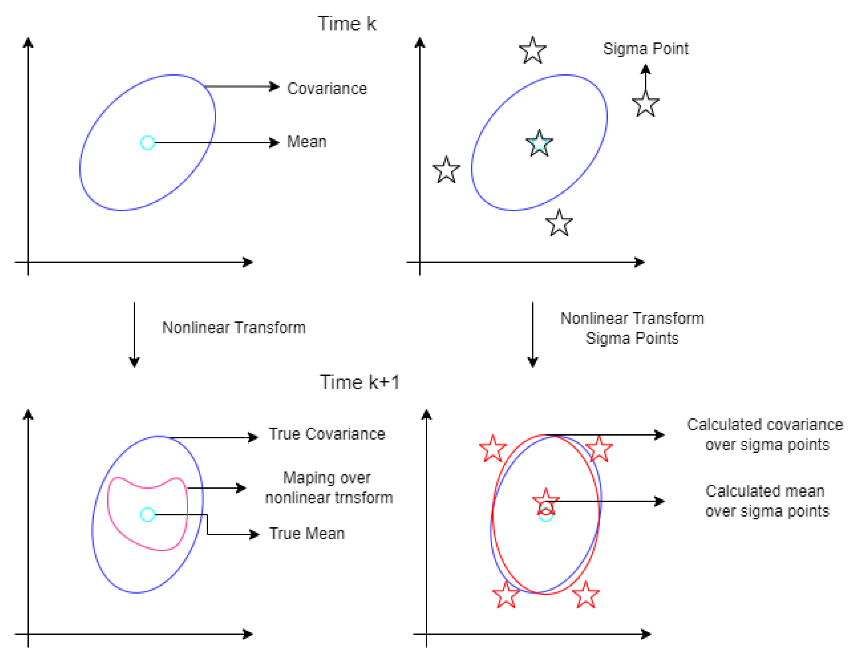
3.2. Unscented Kalman Filter (UKF)

The objective of the UKF is estimating the state $x_k\in {\mathbb{R}}^n$ of the nonlinear stochastic process

$$\begin{array}{c}\hfill \begin{array}{cc}\hfill x_k& =f(x_{k-1},{\eta }_{k-1})\hfill \\ \hfill z_k& =h\left(x_k\right)+{\zeta }_k\hfill \end{array}\end{array}$$

(5)

with the uncorrelated, zero-mean, and normally distributed process and measurement noise ${\eta }_k\in {\mathbb{R}}^q$ and ${\zeta }_k\in {\mathbb{R}}^m$, respectively (i.e., ${\eta }_k\sim \mathcal{N}(0,Q_k)$ and ${\zeta }_k\sim \mathcal{N}(0,R_k)$ hold). To this end, a deterministic sampling approach is employed to approximate the nonlinearities for predicting the estimated state ${\widehat{x}}_k$ and covariance $P_k$ as well as the measurement and cross-covariances $P_{yy}$ and $P_{xy}$ in the measurement update step. Based on these approximations, the basic Kalman filter equations are employed to come up with the corrected estimate [22]. The deterministic sampling makes use of the unscented transform to compute the so-called sigma points (SP) and appropriate weights in order to approximate the probability distribution characterized by their mean and covariance. Compared with the linearization employed in the EKF approach, the sigma points can be subjected to the nonlinear dynamics and measurement equations, enhancing the approximation accuracy [23]. As illustrated in Figure 2 by means of the red and blue ellipsoids, the approximation is very accurate. This error can increase or decrease depending on the sigma point selection method [21,24]. In order to also account for potential nonlinearities affecting the process noise, the augmented state $x_k^a\in {\mathbb{R}}^{n_a}$ with $n_a=n+q$ and covariance, where

$$\begin{array}{c}\hfill \begin{array}{c}{x}_k^a=\left[\begin{array}{c}{x}_k\\ {\eta }_k\end{array}\right],P_k^a=\left[\begin{array}{cc}{P}_k& P_{x\eta ,k}\\ P_{x\eta ,k}& Q_k\end{array}\right]\end{array}\end{array}$$

(6)

as suggested in [21], is employed in the following derivations of the UKF algorithm.

In this paper, a symmetric sigma sampling strategy is used to calculate the SP as in [25] or [26]. Different strategies exist for the number of sigma points [27]. The fusion framework in this paper employs a $2n_a+1$ SP pattern, where a symmetric set of sigma points ${\sigma }_i$ is chosen according to

$$\begin{array}{c}\hfill \begin{array}{c}\hfill {\sigma }_{i,k}=\left\{\begin{array}{cc}{\widehat{x}}_k^a,\hfill & i=0\hfill \\ {\widehat{x}}_k^a+{\left[\sqrt{(n_a+\lambda )P_k^a}\right]}_i,\hfill & i=1,\dots ,n_a\hfill \\ {\widehat{x}}_k^a-{\left[\sqrt{(n_a+\lambda )P_k^a}\right]}_{i-n_a},\hfill & i=n_a+1,\dots ,2n_a\hfill \end{array}\right..\end{array}\end{array}$$

(7)

Here, ${\left[\sqrt{M}\right]}_i$ refers to the ith column of the Cholesky decomposition of the matrix M, which is also applied in [28]. Due to the application of the augmented state vector in Equation (6) and the zero-mean characteristics of the process noise, the mean state in Equation (7) reads as follows:

$${\widehat{x}}_k^a={\left[\begin{array}{cc}{\widehat{x}}_k^T& 0^T\end{array}\right]}^T.$$

(8)

There are different choices [27] for the scalar parameter $\lambda$ that determine how close or far the SPs are from the mean ${\widehat{x}}_k^a$. Within this paper we chose

$$\lambda =3-n_a$$

(9)

Finally, a weight

$$w_i=\left\{\begin{array}{cc}\frac{\lambda }{\lambda +n_a},\hfill & i=0\hfill \\ \frac{1}{2(\lambda +n_a)},\hfill & i=1,\dots ,2n_a\hfill \end{array}\right.$$

(10)

is assigned to each sigma point, which is such that ${\sum }_{i=0}^{2n_a}{w}_i=1$ holds.

In the UKF prediction step, the sigma points are transformed by applying the nonlinear motion model (note that $f^a\left({\sigma }_{i,k-1}\right)$ directly follows from Equation (5) when decomposing the augmented state $x_k^a$ into the original state $x_k$ and the process noise $\eta$${}_k$:

$${\sigma }_{i,k_p}=f^a\left({\sigma }_{i,k-1}\right)$$

(11)

By employing the predicted sigma points, the mean and covariance

$$\begin{array}{c}\hfill \begin{array}{cc}\hfill {\widehat{x}}_{k_p}^a& =\sum _{i=0}^{2n_a}{w}_i{\sigma }_{i,k_p}\hfill \\ \hfill P_{k_p}^a& =\sum _{i=0}^{2n_a}{w}_i({\sigma }_{i,k_p}-{\widehat{x}}_{k_p}^a){({\sigma }_{i,k_p}-{\widehat{x}}_{k_p}^a)}^T\hfill \end{array}\end{array}$$

(12)

are approximated. Figure 2 illustrates the approximations for the simplified example of a two-dimensional state vector $x_k^a$, where five sigma points have been generated.

Once a measurement $z_k$ is obtained, the measurement update step of the UKF is applied. To this end, a predicted measurement

$$z_{i,k_p}=h\left({\sigma }_{i,k_p}\right)$$

(13)

is computed for each sigma point. Based on those predicted measurements, their mean ${\widehat{z}}_{k_p}$ as well as the measurement covariance are computed as follows:

$$\begin{array}{c}\hfill \begin{array}{cc}\hfill {\widehat{z}}_{k_p}& =\sum _{i=0}^{2n_a}{w}_i{z}_{i,k_p},\hfill \\ \hfill P_{yy}& =\sum _{i=0}^{2n_a}{w}_i(z_{i,k_p}-{\widehat{z}}_{k_p}){(z_{i,k_p}-{\widehat{z}}_{k_p})}^T+R_k.\hfill \end{array}\end{array}$$

(14)

By approximating the cross-covariance

$$P_{xy}=\sum _{i=0}^{2n_a}{w}_i({\sigma }_{i,k_p}-{\widehat{x}}_{k_p}^a){(z_{i,k_p}-{\widehat{z}}_{k_p})}^T,$$

(15)

then the Kalman gain

$$\begin{array}{c}\hfill \begin{array}{c}\hfill K=P_{xy}{P}_{yy}^{-1}\end{array}\end{array}$$

(16)

is computed to end up with the updated state and covariance estimate

$$\begin{array}{c}\hfill \begin{array}{cc}\hfill {\widehat{x}}_k^a& ={\widehat{x}}_{k_p}^a+K(z_k-{\widehat{z}}_{k_p}),\hfill \\ \hfill P_k^a& =P_{k_p}^a-K{P}_{yy}{K}^T.\hfill \end{array}\end{array}$$

(17)

3.3. Motion Model

A motion model is employed to predict the state of the objects from time step $k-1$ to k, imposing assumptions regarding the object motion. There are different options in terms of motion models, such as the constant velocity and direction (CV) motion, constant turn rate and acceleration (CTRA), and constant curvature and acceleration models [29]. In terms of calculation effort, the CV model is the best option. It can also be used within a linear Kalman filter, but since it does not encapsulate nonlinear motion, it can be observed that the CV model performs poorly compared with other options in real-life scenarios [29]. Therefore, due to its good ratio between required computational power and performance, the “constant turn rate and velocity” (CTRV) motion model, stated in [29], is employed in Equation (5). Its state vector is

$$x_k={\left[\begin{array}{ccccc}{p}_{x,k}& p_{y,k}& v_k& {\psi }_k& {\dot{\psi }}_k\end{array}\right]}^T$$

(18)

where $p_{x,k}$ and $p_{y,k}$ denote the object’s position in the Cartesian plane relative to the selected origin of the observer. Additional states are the speed $v_k$, the yaw angle ${\psi }_k$ representing the object’s orientation, and the yaw rate ${\dot{\psi }}_k$. Then, the discrete-time nonlinear process model with a sampling period $\Delta t$ reads as follows:

$$x_k=x_{k-1}+\left[\begin{array}{c}\frac{v_{k-1}}{{\dot{\psi }}_{k-1}}\left(sin({\psi }_{k-1}+{\dot{\psi }}_{k-1}\Delta t)-sin\left({\psi }_{k-1}\right)\right)\\ \frac{v_{k-1}}{{\dot{\psi }}_{k-1}}(-cos({\psi }_{k-1}+{\dot{\psi }}_{k-1}\Delta t)+cos\left({\psi }_{k-1}\right))\\ 0\\ {\dot{\psi }}_{k-1}\Delta t\\ 0\end{array}\right]+\left[\begin{array}{c}\frac{1}{2}{\Delta t}^{2}cos\left({\psi }_{k-1}\right){\eta }_{v,k-1}\\ \frac{1}{2}{\Delta t}^{2}sin\left({\psi }_{k-1}\right){\eta }_{a,k-1}\\ \Delta t{\eta }_{a,k-1}\\ \frac{1}{2}{\Delta t}^2{\eta }_{\ddot{\psi },k-1}\\ \Delta t{\eta }_{\ddot{\psi },k-1}\end{array}\right].$$

(19)

Since the CTRV model assumes that the velocity and turn rate are constant, their change between two time steps is zero, and the deterministic part of the equation above is obtained. The process noise vector ${\eta }_k$ is formed by the longitudinal acceleration noise ${\eta }_{a,k}\sim N(0,{\sigma }_a^2)$ and yaw acceleration noise ${\eta }_{{\ddot{\psi }}_k}\sim N(0,{\sigma }_{\ddot{\psi }}^2)$.

3.4. Motion Compensation and Object Association

Ego-motion compensation is a critical part of perception when the sensor carrier can change its speed or orientation. Even a small deviation in the sensor orientation can result in a large variation in the lateral position of an object, depending on the longitudinal distance. This would negatively affect the object association process. Moreover, even in cases where the object association process is successful, the estimation accuracy can be seriously degraded. This happens because the tracked object state vector variables (Equation (18)) are relative to the sensor carrier position and orientation. Therefore, the sensor carrier movements need to be compensated for, and the state vector also needs to be updated before object association and data fusion can be performed. Changes in the sensor carrier state between measurements can be gained via internal sensors or estimated via fusion as shown in [30,31]. Movement compensation is accomplished by means of

$$\left[\begin{array}{c}{x}_{k,p_x}\\ x_{k,p_y}\end{array}\right]=\left[\begin{array}{ccc}cos\left({\dot{\psi }}_{ego}\Delta t\right)& -sin\left({\dot{\psi }}_{ego}\Delta t\right)& {\nu }_{x,ego}\Delta t\\ sin\left({\dot{\psi }}_{ego}\Delta t\right)& cos\left({\dot{\psi }}_{ego}\Delta t\right)& {\nu }_{y,ego}\Delta t\end{array}\right]\left[\begin{array}{c}{x}_{k,p_x}\\ x_{k,p_y}\\ 1\end{array}\right].$$

(20)

After updating the object state vector by means of Equation (19), data association is accomplished with the Hungarian algorithm [32,33]. This algorithm is responsible for linking incoming sensor measurements from different sensors (as object lists) to existing tracked object lists. This is accomplished by computing the distance of each tracked object to each detected object received from the sensor. As an example scenario, when considering tracking an object list with two objects TO1 and TO2 and a new detection list as two objects DO1 and DO2, then the assignment matrix reads as follows:

$$D_{TO,DO}=\left[\begin{array}{cc}{d}_{{TO}_1,{DO}_1}& d_{{TO}_2,{DO}_1}\\ d_{{TO}_1,{DO}_2}& d_{{TO}_2,{DO}_2}\end{array}\right]$$

(21)

where for each entry of the matrix, the object distance to the detected object is calculated by means of the 2D Euclidean distance equation

$$d_{{TO}_u,{DO}_v}=\sqrt{{{(TO}_u.px+{DO}_v.px)}^2+{({TO}_u.py+{DO}_v.py)}^2}$$

(22)

Now, the association problem becomes an optimization problem where the overall cost (i.e., the Euclidean distance between the tracked objects and detected objects) needs to be minimized. The Hungarian algorithm solves this optimization problem and matches the detected objects to tracked objects. It is also applied in order to decide whether a new object track needs to be created or an old one has to be eliminated.

4. Sensor Perception Models

The key components of perception for autonomous vehicles are the sensors. There are two types of sensors used in autonomous vehicles: internal and external sensors. Internal sensors are used to measure the car’s state with an inertial measurement unit (IMU), which consists of an accelerometer, gyroscope, and sometimes also a magnetometer. External sensors are used to perceive the surroundings of the car, such as the distance to an object. Four different sensors are primarily dominant in autonomous vehicles for environmental perception: camera, radar, LiDAR, and ultrasonic sensors. Furthermore, sensors can either be classified as passive sensors or active sensors. Passive sensors receive energy emitted from the surroundings to produce outputs such as RGB or infrared cameras. Active sensors emit energy into the environment (e.g., electromagnetic waves) and measure the reflected waves to produce the output signal, such as LiDAR and radar sensors [15].

The different sensors have their weaknesses and strengths due to their physical measurement principles. For example, a camera needs an external light source (sunlight or streetlights) to operate. In addition, camera performance is very sensitive to weather conditions such that on a foggy day, its detection range is reduced. As with cameras, LiDAR is also affected by weather conditions. On the one side, LiDAR provides very accurate distance measurement, but on the other side, the spatial resolution of LiDAR is limited compared with high-definition cameras. Especially at a long range, fewer details are measured for object detection and classification. In contrast, radar is relatively unaffected by weather conditions and does not suffer at long ranges as LiDAR does, but generally, it has a low spatial resolution. Therefore, radar clusters do not contain much information for object classification, unlike a LiDAR point cloud or a camera image. Considering the given examples, a sensor fusion method should address the weaknesses of each sensor and make the perception process more reliable. In this paper, internal sensors and external sensors, namely cameras, LiDAR, and radar, are used within the data fusion framework.

For generating data, the LGSVL simulator from LG Electronics America R&D Lab is used in this paper. The LGSVL simulator provides a highly realistic 3D environment for simulating autonomous vehicles and robotic applications [34]. It is also possible to receive the ground truth by simulation to compare it with the results of the detection algorithm. The ground truth information from the simulation is also used for the generation of the object list. In the simulation, the ground truth sensor is placed on the vehicle. Using the ground truth sensor, the object type, location, and volume information (i.e., a 3D bounding box) can be gathered without any noise. To convert the ground truth data to respective sensor detection, a 3D point is selected from the 3D bounding box, and its position relative to the sensor is calculated. In this paper, the location of the 3D point is selected at the bottom-middle (Figure 3) of the total visible volume. Since the received object location is relative to the ground truth sensor, each simulated perception sensor has a ground truth sensor in it. To generate a realistic object list from the ground truth, sensor models have to be implemented for each sensor, which will be explained in the following subsections.

4.1. Camera

Cameras are widely applied in vehicles for various applications, such as in autonomous driving assistant systems (ADASs) (e.g., emergency braking), because they provide high-resolution data and are low in cost. Vehicles’ perception cameras are mainly used for lane detection, traffic sign detection, object detection, etc. There are also use cases for employing cameras in vehicles for human–machine interaction [35]. Furthermore, cameras are also used to improve the detection capabilities of other sensors such as LiDAR and radar [36]. One of the major drawbacks of the camera sensor is the computational power needed for processing the image data. Cameras can produce millions of pixels per frame with a high frame rate. This leads to multiple megabytes of data processing in real time [16]. Another disadvantage is that cameras lack native depth information. Although depth information can be calculated, it requires additional computational power, and the accuracy of the depth information is limited, depending on the applied method [37].

In order to generate a synthetic object list in the form of camera object detection, the 3D bounding boxes received from the LGSVL simulation are converted to image coordinates by the following equation (more information in [38], page 6, Equation (1)):

$$z_{camer{a}_k}=w\left[\begin{array}{c}u\\ v\\ 1\end{array}\right]=KT{\left[XYZ1\right]}^T$$

(23)

In Equation (23), w is a scalar and K is a 3 × 3 matrix representing the intrinsic camera parameters. T = [Rt] is a 3 × 4 matrix representing the rotation (R) and translation (t) of the camera, depending on the world coordinate system. Lastly, the 3D point (i.e., bottom-middle point of the 3D bounding box) is represented as a 4 × 1 vector. Equation (23) is used for each object received from the ground truth sensor in the process of converting the object position to the camera coordinate system. After that, additional random noise is added to each object location in the pixel coordinate system. In this paper, up to four-pixel noise is applied using a random uniform distribution in both lateral and longitudinal locations.

In a real-life scenario, an object detection algorithm delivers objects as 2D or 3D bounding boxes. In both cases, a point which can be also extracted by other cooperative sensors should be selected, since the developed sensor fusion algorithm requires a single point for fusion. As an example, for image-based detection and classification, YOLOv4 [39] can be used. The YOLOv4 object list consists of objects with each object location represented as 2D bounding boxes. In order to use this information in the fusion framework, the middle-bottom point is selected from each bounding box. The error in the measurement parameter should be selected by considering two factors. In the case of using only the camera sensor, the only error sources are the shape of the bounding box and how well the box encapsulates the detected object. In the case of multi-sensor fusion, the measurement error should also include a point selection error. For example, the vehicle tracking point is at the middle-bottom, and due to the orientation of the car, the detected bounding box’s middle-bottom is not the same as the original tracking point. This phenomenon applies to all other sensors discussed in the following sections.

4.2. LiDAR

LiDAR is an active sensor that emits pulses to the environment which are reflected by objects. With these reflections, the time of flight of the laser beam is measured between the emission and reception of the light pulse, which enables calculation of the distance. As an active sensor, LiDAR is relatively robust under different lighting conditions (e.g., day or night, glare, or shadows) [40]. However, depending on the laser beam frequency, the signal-to-noise (SNR) ratio can be reduced by strong sunlight exposure. In terms of the perception task, LiDAR can be placed in between the camera and the radar. In terms of object classification, LiDAR does not provide a high resolution compared with a camera. However, in terms of 3D localization, LiDAR provides an extremely high spatial resolution of objects without significant backend processing compared with radar. Aside from perception tasks, LiDAR is also used for high-definition maps and the generation of urban models for reliable localization and referencing [36]. To generate a synthetic object list, a ground truth sensor is used. Since the ground truth sensor provides the location of an object in a Cartesian coordinate system, there is no need for extra conversion. To make the object list more realistic when testing the fusion from −0.15 m to +0.15 m (random uniform distribution), noise was added to both the lateral and longitudinal distances for every received object. In a real-life scenario, an object detection algorithm would deliver a 3D bounding box, such as a point RCNN [41], or a cluster of points where the object is located, such as the Autoware.ai LiDAR Euclidean cluster detection algorithm [42]. As an example, for LiDAR-based detection, the Euclidean clustering method can be used. This algorithm provides an object list, where every object is represented by multiple points. For each detected object, the closest point to the sensor can be selected from the point cluster for the rest of the fusion process.

4.3. Radar

Automotive radars are used to detect the velocity and range of road participants around the vehicle. An automotive radar uses radio waves and consists of a transmitter and a receiver. The transmitter sends out radio waves which are reflected by objects back to the receiver. The sensor determines the object’s distance, velocity, and direction by digital signal processing. It uses the Doppler effect to determine the relative radial speed of the objects. For perception, radar is mainly used for receiving object position and velocity information. Although radar has a low resolution in terms of object classification and lower quality in terms of lateral distance estimation compared with cameras and LiDAR, it has unique properties such as long-range detection, a relative speed, and the capability to function irrespective of illumination conditions. Therefore, radar is a popular sensor in autonomous driving technologies.

A point in Cartesian coordinates can be converted to a radial radar cluster point with the following equation:

$$z_{rada{r}_k}=\left[\begin{array}{c}Range\\ Bearing\\ RangeRate\end{array}\right]=\left[\begin{array}{c}\sqrt{p_x^2+p_y^2}\\ arctan\frac{p_y}{p_x}\\ \frac{p_x{v}_x+p_y{v}_y}{\sqrt{p_x^2+p_y^2}}\end{array}\right]$$

(24)

In Equation (24), $p_x$ and $p_y$ are 2D object locations in a Cartesian coordinate system, and $v_x$ and $v_y$ are the speeds in the $p_x$ and $p_x$ directions of the object, respectively. Equation (24) is used for each object received from the ground truth sensor in the process of converting the object’s position and velocity to the radar cluster. After that, additional random noise is added to each object. The added noise (random uniform distribution) ranges are as follows: +−0.3, +−0.03, and +−0.3 for the range, bearing (radian), and radial velocity, respectively.

In a real-life scenario, an object detection algorithm would deliver a cluster point or multiple cluster points for an object. As an example, for radar-based detection, a DBSCAN algorithm can be used [43]. This algorithm gives an object list, where every object has one or more radar points. For each detected object where there is more than one point representing the object, as in the case of LiDAR, the closest point to the sensor that can be selected from the point cluster for the rest of the fusion process is taken.

5. Simulation and Experiment Results

5.1. Simulation Results

In order to validate the developed data fusion framework in different scenarios, the LGSVL simulation tool was used. In the simulation, the artificial sensors (i.e., radar, LiDAR, and cameras) were located at different positions of the sensor carrier car to generate sensor data. Different noise values were added to the ground truth as explained in the previous section. In this section, one specific scenario is presented. In the scenario, one vehicle (referred to as the ego car) was equipped with sensors, and it detected and tracked other objects (i.e., targets), such as Target Car 2 (TC2), Target Car 3 (TC3), and Target Car 4 (TC4). The trajectories of the ego car and the targets are depicted in Figure 4b. The ego car was driving straight for a while in the right lane, as shown in Figure 4a, and made a right turn, similar to TC3. TC4 was driving in the opposite direction of the ego car, and TC2 and TC3 were driving in the same direction. For the scenario, the frame-by-frame results can be seen in Figure 5, and the root mean square error (RMSE) results can be seen in

Table 1. The first group of columns is the result of the fusion for each individual car when all the sensors were in use. The second group of columns is the result of the fusion when employing different combinations in the sensor set for Target Car 3. The root mean square error (RMSE) values for both scenarios and every tracked object are shown, where the RMSE is the standard deviation of the residuals (prediction error). Here, cm = centimeter, m/s: meters per second, L = LiDAR, R = radar, C = camera, L+R = LiDAR and Radar used at same time, etc.

	Scenario One (All Sensors)			Target Car 3 (Different Sensor Combinations)
Target Car Name	TC2	TC3	TC4	L + R	L + C	R + C	L	R	C
RMSE in Longitudinal Distance (cm)	6.7	7.0	7.4	6.9	8.9	12.6	8.1	10.8	43
RMSE in Lateral Distance (cm)	6.1	4.8	7.3	7.0	4.7	5.4	7.2	19.7	5.2
RMSE in Velocity (m/s)	0.27	0.21	0.53	0.21	0.68	0.25	0.67	0.18	0.99

. Additionally, in Table 1, the results of the fusion framework are depicted for when different sensor combinations were employed. As can be seen from the RMSE values, individual sensor failure during operation time would not be fatal to the developed sensor fusion framework. Another observation from the table is that when using different combinations of the sensor set, the individual sensors might give closer results to the ground truth with respect to the location and speed. For example, in the case of using only the radar sensor, the velocity estimation was better than when using all three sensors. This is because every attribute in the object state is connected by the motion model, which is explained in Section 3.3. When the filter updates its states, it will try to get closer to the most trusted attribute of the measurement. In the case of radar, which provided the location and speed of the object, the trustworthiness of the speed value was higher. Therefore, the filter would tend to get closer to the measured speed value and update the location value to fit the speed information.

5.2. Possible Inaccuracies of the Detection Algorithms

In

Table 2. The first group of columns shows the effect of undetected objects on the data fusion, and the second group of columns shows the effect of the measurement error in detection. In the first scenario, the target cars were used for both tests, and the results are produced by using all sensors, as in Table 1.

	Missing Detection			Error in the Detection
Target Car Name	TC2	TC3	TC4	TC2	TC3	TC4
RMSE in Longitudinal distance (cm)	11.4	12.7	10.5	10.7	14.2	13.4
RMSE in Lateral distance (cm)	8.3	7.2	8.1	15.4	15.1	19.0
RMSE in Velocity (m/s)	0.44	0.31	0.42	0.33	0.29	0.66

, the results are presented for a missing detection scenario, where some of the objects in the field of view were not detected by the simulated detection algorithm. For this scenario, in the object list generation phase, after receiving the ground truth object list from the respective sensor, some of the objects were randomly removed from the object list. In this test case, every detected object had a predefined percentage staying in the object list. The predefined percentage of staying in the object list for each sensor was as follows: camera = 80%, LiDAR = 60%, and radar = 60%. The fusion results for the missing detection case are shared in Table 2. Although reducing the number of detections reduced the fusion accuracy, the results did not significantly deviate from the results presented in Table 1.

Another source of inaccuracy in the fusion is caused by point selection. Due to the nature of the simulation environment, one can select a single 3D point from the object (bottom-middle, center, etc.) that represents the object’s location, and the same point on the object can be selected for the other mentioned sensors precisely. For example, when considering a sedan car as a detected object from behind, the height of the object is approximately 1.5 m, and the width of the object is approximately 1.8 m. Although current detection algorithms are getting better every day, it is still a challenging task to select the same point in around a 2.8 square meter area for all the sensors. Therefore, one needs to realize that in a real-life scenario, the results can be different from the simulation results if the detection algorithm does not provide robust detection. When considering detection from behind the car, selecting the same point with different sensors is more important for lateral distance estimation than longitudinal distance estimation. The position of the selected 3D point does not affect the longitudinal distance estimation excessively since there is not much variety regarding depth in a 2.7 square meter area. For this scenario, when generating the object list from each sensor, two different types of noise are added to the ground truth measurement. The first noise is the previously mentioned sensor noise, which was used in the previous test cases with the same numerical values. However, before applying sensor noise, this time, detection errors in terms of 3D point selection were also applied. For every detection, as detection error, noise (random uniform distribution) between 0.5 m in the lateral and from 0 to 0.2 m in the longitudinal axis was applied. As expected, this change in the object list generation phase reduced the accuracy of the fusion result (Table 2). The point selection error can be further reduced by considering the object viewing angle of the sensor in real-life scenarios.

5.3. nuScenes Results

In addition to the simulation, the nuScenes dataset [44] was used to demonstrate the performance of the proposed fusion algorithm on real data. Because this paper did not focus on individual sensor detection algorithms, well-known algorithms were used. For image-based detection and classification, we used YOLOv4 [39]. For LiDAR detection, Autoware.ai lidar Euclidean cluster detection was used [42]. Lastly, for radar detection, DBSCAN was used as described in the sensor (Section 4). The implemented fusion framework aims to also work with noisy observations (e.g., double detection of an object, ghost object detection, and missing detections). Some modern, more advanced detection algorithms would outperform the selected detection algorithms by far, and the noise would be significantly reduced. Therefore, in this paper, the overall tracking results (e.g., the AMOTA metric) were not calculated, since the performance of the fusion framework was significantly affected by the used detection algorithms. The goal of the demonstration was to show that by applying the methodology presented in this paper, the detection accuracy of the fused objects would increase. For the validation, only one target car (i.e., the white van and red sedan) was selected for two different scenes (see Figure 6a,c). In the video sequence of the white van, although the dataset contained more than 200 images of the white van, only 34 annotations were provided (i.e., hand-labeled information such as the position and 3D bounding box). The detection algorithms were applied to all the available sensor data, and the results of the framework were compared with the annotations (see Figure 6b). As can be seen in Figure 6b, the deviation between the predicted position and ground truth position was larger than that obtained within the simulation (Table 2), which was due to the fact that the ground truth position (i.e., a point in the target car) was not always the same as the tracking point. In addition, the hand-labeled 3D bounding box locations varied between frames in the previously mentioned 34 annotated frames. Nevertheless, as can be seen in Figure 6b,d, the fusion framework provided a more robust localization than any individual sensor.

6. Sensor Fault Detection

Object list-based data fusion frameworks have the advantage that individual sensor failures do not lead to a complete perception failure, but only less accurate detections and localizations are obtained. In addition to that, they provide the opportunity to identify potential malfunctions in sensors. The new concept of fault detection developed in this paper is based on the identification of anomalies in the signal of one sensor in reference to the other sensor signals. The approach to identifying a potential failure depends on the failure mode. Therefore, one needs to first distinguish the different failure modes. There are failures due to slow wear-out phenomena which cause a slow change in the sensor performance on a relatively long timescale (e.g., years or months), and there are spontaneous failures where the sensor stops delivering data on a second or sub-second timescale. Examples of slow degradation due to wear-out are a reduction in range due to the degrading output power of the light-emitting laser for a LiDAR sensor, a reduction in the signal-to-noise for a radar sensor due to the degradation of the HF chip, and a reduction in sharpness for a camera due to degradation of the objective [45]. In addition, the mounting position of a sensor (e.g., the orientation of the sensor) might shift, and therefore, the extrinsic calibration parameters of the sensor change. These mechanical changes can progress slowly but also spontaneously if an impact occurs. In addition, soiling of the sensor can cause a very fast sensor performance change or progress on a slow timescale. Other spontaneous failures can include catastrophic electronic failures. The different failures can be identified with the help of the multi-sensor fusion framework using the known accuracies of the sensors within standard scenarios. For example, under appropriate weather conditions, the motorway camera, LiDAR and radar are able to detect a specific car at a specific distance according to their well-defined specifications. Initially, all sensors are calibrated to the car coordinate system and to each other through that. If the detection from one of the sensors repeatedly deviates during a lifetime in such a defined situation from the results of the other sensors, then action can be taken as soon as the number of occurrences in a time interval, and the magnitude of deviation exceeds a chosen threshold value. One action is, for instance, the recalibration of the extrinsic parameters of the sensor when a constant shift of one sensor to the other sensors is identified. Another example is the range of the LiDAR sensor. In standard defined situations, LiDAR object detection performance at long ranges can be continuously compared with the other sensors (e.g., with radar) to identify a possible reduction in the detection range. Aside from the described examples of malfunctioning detection of sensors in the system, detection algorithm-based errors can also be identified. In case of the unexpected missing object detection of one sensor, the region of interest (ROI) can be focused on for the sensor in the area where the object is missing. In other words, the ROI can be used to support the detection algorithm when the sensor fails to detect an object but other sensors do. If the camera, for example, does not detect an object, and if the focus of the ROI also does not improve the detection in a standard situation, then the framework will give a warning to the user about possible blocking of the field of view of the camera due to dirt or scratches. Many more specific algorithms can be developed to support self-diagnostics in multi-sensor systems. Depending on the kind of malfunction, counteractions can be realized (e.g., recalibration). Furthermore, sensor degradation can be identified, and maintenance can be scheduled in time before catastrophic sensor failure. In future works, the developed algorithms will be evaluated in practice to enable the functional safety of the sensors for environmental perception.

7. Conclusions and Future Works

In this paper, a new efficient sensor fusion framework was presented, and its results were demonstrated in a simulated environment and experimentally using the nuScenes dataset. The fusion framework enabled the efficient fusion of sensor data at the object level and could provide autonomous vehicles with a robust map of the environment. It operates independently from the type and number of sensors and allows the flexible integration of new sensors. Depending on the requirements and use case, different sensor configurations can be selected. Failure of one sensor during operation will not result in a system failure, as that might happen in raw-level fusion but will only cause a reduction in object position accuracy. Furthermore, the same framework can be used in moving coordinate systems, such as vehicles, or in static roadside infrastructure (e.g., sensor units on public roads) for surveillance and smart city applications. Furthermore, a new concept was developed to detect hardware- or software-based malfunctions by using the high-level fusion framework (i.e., using the other sensors in operation as a reference). The developed algorithms will be evaluated in the field to improve the functional safety of the sensor system for environmental perception.

References

1. Galvao, L.G.; Abbod, M.; Kalganova, T.; Palade, V.; Huda, M.N. Pedestrian and Vehicle Detection in Autonomous Vehicle Perception Systems—A Review. Sensors 2021, 21, 7267. [Google Scholar] [CrossRef] [PubMed]
2. Llinas, J.; Hall, D.L. An introduction to multisensor data fusion. Proc. IEEE 1997, 85, 6–23. [Google Scholar]
3. Chen, X.; Ma, H.; Wan, J.; Li, B.; Xia, T. Multi-View 3D Object Detection Network for Autonomous Driving. In Proceedings of the IEEE Conference on Computer Vision and Pattern Recognition, Honolulu, HI, USA, 21–26 July 2017. [Google Scholar]
4. Kaempchen, N.; Buehler, M.; Dietmayer, K. Feature-level fusion for free-form object tracking using laserscanner and video. In Proceedings of the IEEE Intelligent Vehicles Symposium, Las Vegas, NV, USA, 6–8 June 2005. [Google Scholar]
5. Floudas, N.; Polychronopoulos, A.; Aycard, O.; Burlet, J.; Ahrholdt, M. High Level Sensor Data Fusion Approaches For Object Recognition. In Proceedings of the IEEE Intelligent Vehicles Symposium, Istanbul, Turkey, 13–15 June 2007. [Google Scholar]
6. Michaelm, A.; Nico, K. High-Level Sensor Data Fusion Architecture for Vehicle Surround Environment Perception. In Proceedings of the 8th International Workshop on Intelligent Transportation, Hamburg, Germany, 22–23 March 2011. [Google Scholar]
7. Li, W.; Wang, Z.; Wei, G.; Ma, L.; Hu, J.; Ding, D. A Survey on Multisensor Fusion and Consensus Filtering for Sensor Networks. Discret. Dyn. Nat. Soc. 2015, 2015, 683701. [Google Scholar] [CrossRef]
8. Chen, H.; Kirubarajan, T.; Bar-shalom, Y. Performance limits of track-to-track fusion versus centralized estimation: Theory and application. IEEE Trans. Aerosp. Electron. Syst. 2003, 39, 386–400. [Google Scholar] [CrossRef]
9. Premebida, C.; Monteiro, G.; Nunes, U.; Peixoto, P. A Lidar and Vision-based Approach for Pedestrian and Vehicle Detection and Tracking. In Proceedings of the IEEE Intelligent Transportation Systems Conference, Seattle, WA, USA, 30 September–3 October 2007. [Google Scholar]
10. Zhang, F.; Clarke, D.; Knoll, A. Vehicle Detection Based on LiDAR and Camera Fusion. In Proceedings of the International IEEE Conference on Intelligent Transportation Systems (ITSC), Qingdao, China, 8–11 October 2014. [Google Scholar]
11. Wang, X.; Xu, L.; Sun, H.; Xin, J.; Zheng, N. On-Road Vehicle Detection and Tracking Using MMW Radar and Monovision Fusion. IEEE Trans. Intell. Transp. Syst. 2016, 17, 2075–2084. [Google Scholar] [CrossRef]
12. Gohring, D.; Wang, M.; Schnurmacher, M.; Ganjineh, T. Radar/Lidar Sensor Fusion for Car-Following on Highways. In Proceedings of the International Conference on Automation, Robotics and Applications, Wellington, New Zealand, 6–8 December 2011. [Google Scholar]
13. Shahian Jahromi, B.; Tulabandhula, T.; Cetin, S. Real-Time Hybrid Multi-Sensor Fusion Framework for Perception in Autonomous Vehicles. Sensors 2019, 19, 4357. [Google Scholar] [CrossRef] [PubMed]
14. Luiten, J.; Fischer, T.; Leibe, B. Track to Reconstruct and Reconstruct to Track. IEEE Robot. Autom. Lett. 2020, 5, 1803–1810. [Google Scholar] [CrossRef]
15. Yeong, D.J.; Velasco-Hernandez, G.; Barry, J.; Walsh, J. Sensor and Sensor Fusion Technology in Autonomous Vehicles: A Review. Sensors 2021, 21, 2140. [Google Scholar] [CrossRef] [PubMed]
16. Kocić, J.; Jovičić, N.; Drndarević, V. Sensors and Sensor Fusion in Autonomous Vehicles. In Proceedings of the Telecommunications Forum (TELFOR), Belgrade, Serbia, 20–21 November 2018; pp. 420–425. [Google Scholar]
17. Kalman, R.E. A new approach to linear filtering and prediction problems. J. Fluids Eng. 1960, 82, 35–45. [Google Scholar] [CrossRef]
18. Li, Q.; Li, R.; Ji, K.; Dai, W. Kalman Filter and Its Application. In Proceedings of the International Conference on Intelligent Networks and Intelligent Systems (ICINIS), Tianjin, China, 1–3 November 2015. [Google Scholar]
19. Welch, G.; Bishop, G. An Introduction to the Kalman Filter. Available online: https://www.cs.unc.edu/~welch/media/pdf/kalman_intro.pdf (accessed on 16 January 2023).
20. Fujii, K. Extended Kalman Filter. Tech. rep. The ACFA-Sim-J Group. 2003. Available online: https://www-jlc.kek.jp/2004sep/subg/offl/kaltest/doc/ReferenceManual.pdf (accessed on 16 January 2023).
21. Julier, S.J.; Uhlmann, J.K. New extension of the kalman filter to nonlinear systems. In Proceedings of the Signal Processing, Sensor Fusion, and Target Recognition VI, Orlando, FL, USA, 21–24 April 1997; pp. 182–193. [Google Scholar]
22. Wan, E.A.; Van Der Merwe, R. The unscented Kalman filter for nonlinear estimation. In Proceedings of the IEEE 2000 Adaptive Systems for Signal Processing, Communications, and Control Symposium, Lake Louise, AB, Canada, 4 October 2000. [Google Scholar]
23. Sakai, A.; Tamura, Y.; Kuroda, Y. An Efficient Solution to 6DOF Localization Using Unscented Kalman Filter for Planetary Rovers. In Proceedings of the IEEE/RSJ International Conference on Intelligent Robots and Systems, St. Louis, MO, USA, 10–15 October 2009. [Google Scholar]
24. Julier, S.J. The spherical simplex unscented transformation. In Proceedings of the 2003 American Control Conference, Denver, CO, USA, 4–6 June 2003. [Google Scholar]
25. Jeon, D.; Choi, H.; Kim, J. UKF data fusion of odometry and magnetic sensor for a precise indoor localization system of an autonomous vehicle. In Proceedings of the 13th International Conference on Ubiquitous Robots and Ambient Intelligence (URAI), Xian, China, 19–22 August 2016. [Google Scholar]
26. Anjum, M.L.; Park, J.; Hwang, W.; Kwon, H.I.; Kim, J.H.; Lee, C.; Kim, K.S. Sensor data fusion using Unscented Kalman Filter for accurate localization of mobile robots. In Proceedings of the ICCAS 2010, Gyeonggi-do, Republic of Korea, 27–30 October 2010. [Google Scholar]
27. Kokkala, J.; Solin, A.; Särkkä, S. Sigma-Point Filtering Based Parameter Estimation in Nonlinear Dynamic Systems. J. Adv. Inf. Fusion 2015, 11, 15–30. [Google Scholar]
28. Cholesky, A.-L. Note sur une méthode de résolution des équations normales provenant de l’application de la méthode des moindres carrés à un système d’équations linéaires en nombre inférieur à celui des inconnues (Procédé du Commandant Cholesky). Bull. Géod. 1924, 2, 67–77. [Google Scholar]
29. Schubert, R.; Richter, E.; Wanielik, G. Comparison and evaluation of advanced motion models for vehicle tracking. In Proceedings of the 11th International Conference on Information Fusion, Cologne, Germany, 30 June–3 July 2008. [Google Scholar]
30. Liu, W.; Xia, X.; Xiong, L.; Lu, Y.; Gao, L.; Yu, Z. Automated Vehicle Sideslip Angle Estimation Considering Signal Measurement Characteristic. IEEE Sens. J. 2021, 21, 21675–21687. [Google Scholar] [CrossRef]
31. Liu, W.; Xiong, L.; Xia, X.; Lu, Y.; Gao, L.; Song, S. Vision-aided intelligent vehicle sideslip angle estimation based on a dynamic model. IET Intell. Transp. Syst. 2020, 14, 1183–1189. [Google Scholar] [CrossRef]
32. Kuhn, H.W. The Hungarian method for the assignment problem. Nav. Res. Logist. Q. 1955, 2, 83–97. [Google Scholar] [CrossRef]
33. Sahbani, B.; Adiprawita, W. Kalman filter and Iterative-Hungarian Algorithm implementation for low complexity point tracking as part of fast multiple object tracking system. In Proceedings of the 6th International Conference on System Engineering and Technology (ICSET), Bandung, Indonesia, 3–4 October 2016. [Google Scholar]
34. Rong, G.; Shin, B.H.; Tabatabaee, H.; Lu, Q.; Lemke, S.; Boise, E.; Uhm, G.; Gerow, M.; Mehta, S.; Agafonov, E.; et al. LGSVL Simulator: A High Fidelity Simulator for Autonomous Driving. arXiv 2020, arXiv:2005.03778. [Google Scholar]
35. Fridman, L. Human-Centered Autonomous Vehicle Systems: Principles of Effective Shared Autonomy. arXiv 2018, arXiv:1810.01835. [Google Scholar]
36. Li, Y.; Ma, L.; Zhong, Z.; Liu, F.; Chapman, M.A.; Cao, D.; Li, J. Deep Learning for LiDAR Point Clouds in Autonomous Driving: A Review. IEEE Trans. Neural Netw. Learn. Syst. 2020, 32, 3412–3432. [Google Scholar] [CrossRef]
37. Bhoi, A. Monocular Depth Estimation: A Survey. arXiv 2019, arXiv:1901.09402. [Google Scholar]
38. Kumar, G.A.; Lee, J.H.; Hwang, J.; Park, J.; Youn, S.H.; Kwon, S. LiDAR and Camera Fusion Approach for Object Distance Estimation in Self-Driving Vehicles. Symmetry 2020, 12, 324. [Google Scholar] [CrossRef] [Green Version]
39. Bochkovskiy, A.; Wang, C.Y.; Liao, H.Y.M. YOLOv4: Optimal Speed and Accuracy of Object Detection. arXiv 2020, arXiv:2004.10934. [Google Scholar]
40. Wu, B.; Wan, A.; Yue, X.; Keutzer, K. SqueezeSeg: Convolutional Neural Nets with Recurrent CRF for Real-Time Road-Object Segmentation from 3D LiDAR Point Cloud. In Proceedings of the IEEE International Conference on Robotics and Automation (ICRA), Brisbane, QLD, Australia, 21–25 May 2018; pp. 1887–1893. [Google Scholar]
41. Shi, S.; Wang, X.; Li, H. PointRCNN: 3D Object Proposal Generation and Detection From Point Cloud. In Proceedings of the IEEE Conference on Computer Vision and Pattern Recognition (CVPR), Long Beach, CA, USA, 15–20 June 2019. [Google Scholar]
42. Autoware. AI. Autoware: Open-Source Software for Urban Autonomous Driving; The Autoware Foundation: Nagoya, Japan, 2019. [Google Scholar]
43. Kellner, D.; Klappstein, J.; Dietmayer, K. Grid-based DBSCAN for clustering extended objects in radar data. In Proceedings of the 2012 IEEE Intelligent Vehicles Symposium, Madrid, Spain, 3–7 June 2012. [Google Scholar]
44. Caesar, H.; Bankiti, V.; Lang, A.H.; Vora, S.; Liong, V.E.; Xu, Q.; Krishnan, A.; Pan, Y.; Baldan, G.; Beijbom, O. nuScenes: A multimodal dataset for autonomous driving. In Proceedings of the IEEE Conference on Computer Vision and Pattern Recognition (CVPR), Seattle, WA, USA, 13–19 June 2020. [Google Scholar]
45. Kettelgerdes, M.; Böhm, L.; Elger, G. Correlating Intrinsic Parameters and Sharpness for Condition Monitoring of Automotive Imaging Sensors. In Proceedings of the 5th International Conference on System Reliability and Safety (ICSRS), Palermo, Italy, 24–26 November 2021. [Google Scholar]
Figure 1. (a) Proposed N sensor perception node flow chart. The data fusion method and CTRV are explained in Section 2 and Section 3, respectively. Object association and motion compensation are explained in Section 4. Object detection and classification methods are not in the scope of this paper. The object detection algorithm used in the experimental validation is explained in Section 4. (b) Fault detection node (detailed in Section 6).
Processes 11 00501 g001
Figure 2. Unscented transform process: selecting sigma points and calculating posterior covariance and mean after transformation.
Processes 11 00501 g002
Figure 3. On the left side, a 3D bounding box is constructed based on the road user projected on the image plane. On the right side, green, red, and yellow represent the back, front, and bottom of the object, respectively. When the detection algorithm of a sensor provides a 3D bounding box, in general, any point in the 3D box can be selected as the detected position of the traffic user. For object list-based sensor fusion, however, it needs to be ensured that the different sensors deliver an object list where the same position can be extracted.
Processes 11 00501 g003
Figure 4. (a) LGSV L simulation front camera view starting position of the scenario. (b) Scenario from the start to the end of the simulation, with car trajectories for ego and target cars. In this scenario, the ego followed Target Car 3.
Processes 11 00501 g004
Figure 5. Frame-by-frame comparison between tracking results and ground truth for the first scenario. In the XY position graph, green, pink, and yellow are generated LiDAR, radar, and camera measurements, respectively. Radar (polar coordinate system) and camera (pixel coordinate system) measurements were converted to the Cartesian coordinate system for visualization purposes.
Processes 11 00501 g005
Figure 6. (a,c) Front camera view of nuScenes dataset, where x (longitudinal) and y (lateral) are relative distances from the ego car position. (Positional information text was removed from persons for better readability.) (b) Frame-by-frame comparison between tracking results and ground truth for the white van seen in the image. (d) Frame-by-frame comparison between tracking results and ground truth for red sedan seen in the image.
Processes 11 00501 g006