Abstract
The purpose of this article is to point out the need to use software simulation tools in industrial practice to optimize the production process and assess the economic effectiveness of investment, including risk. The goal of the research is to find an optimal investment variant to ensure an increase in the production volume of at least 50% and to achieve the maximum economic efficiency of the investment, even considering the risk. The article presents a comprehensive approach that enables the achievement of the set research goal. The selection of the optimal version of the investment is carried out in three steps. Firstly, the versions of the investment variants are assessed from the production point of view using the program Tecnomatix Plant Simulation. Subsequently, the versions of the investment variants are assessed from an economic point of view and from a risk point of view. Economic efficiency is assessed using the financial criteria net present value (NPV), profitability index (PI), and discounted payback period (DPP), and risk analysis is carried out using Monte Carlo simulations. Finally, the accepted outputs are evaluated overall using a multi-criteria method, namely the method of partial order.
1. Introduction
The investment activity of enterprises, especially investments in production technologies, is a necessary condition for the competitive ability of a production company. Decision-making about investments belongs to strategic decisions, and therefore should be supported by a thorough analysis of production possibilities and production capacity utilization, as well as an analysis of the economic efficiency of the investment, including risk. Several research works deal with the issue of investment decision-making in various aspects. A research work by Freiberg and Scholz [1] presented a comprehensive analysis of the benefits generated by actual investment in modern manufacturing equipment covering all relevant effects related to the investment. A frequent subject of research works on this topic is production optimization aimed at balancing production lines. For example, in a paper by Aguilar et al. [2], parallel assembly lines balancing problem (PALBP) studies were surveyed. Likewise, Van Hop [3] addressed the mixed-model line balancing problem with fuzzy processing time. They developed a fuzzy heuristic to solve the problem based on aggregating fuzzy numbers and combined precedence constraints. In the study by [4], the factors that affect the implementation of intelligent systems in motor production lines were analyzed. The implementation of intelligent systems is heading toward Industry 4.0. In view of Industry 4.0, Zhao et al. [5] also utilized the semi-physical simulation technology of digital twins to verify a proposed design scheme to achieve the balance optimization of a production line. Daneshjo and Malega presented in [6] the usage of automation in an improvement project for the Cinematic production line. A study by [7] proposed an approach to simultaneously designing products and processes by integrating assembly line balancing, design, and sensitivity analysis of assembly line design. Lu and Yang [8] proposed an approach for solving integrated assembly sequence planning and assembly line balancing with an ant colony algorithm. The research conducted by Liu et al. [9] utilized uncertainty theory to model uncertain demand. The uncertain demand was described using scenario probability and triangular fuzzy numbers. Finally, a new optimization model for mixed-model assembly line balancing was established. In a further publication, Kalayci et al. [10] presented a fuzzy extension of the disassembly line balancing problem with fuzzy task processing times. In a paper by [11], a heuristic assembly line balancing procedure was used to solve the limitations of maximum working team numbers in assembly line stations. The workload smoothness of assembly lines was the subject of further research. The authors proposed an algorithm to solve a two-sided assembly line balancing problem [12] and developed linear mathematical models to assign tasks to the stations of an assembly line [13]. Fathi et al. [14] investigated the efficiency of performance measures for minimizing the number of workstations in approaches addressing assembly line balancing problems for both straight and U-shaped lines. Similarly, using the branch and bound algorithm, a simple assembly line balancing problem was solved by Azizoğlu and İmat [15].
In decision-making processes about investments in production equipment, software tools designed for production process modelling and simulations are a great help. Through simulations, it is possible to review production capacities in a virtual environment, assess their utilization, and thus improve the quality of investment decisions. In this area, e.g., Chai et al. [16] published their experience with software tools for production process simulation. In their study, a production line 3D visualization monitoring system based on OpenGL modelling was established on a VC++6.0 platform. Production line 3D visualization provided production capacity simulation to optimize the parameter settings. Research on an assembly line using the Arena Simulation program to address the balancing problem was performed by Kayar and Akalin [17]. Likewise, to address the balancing issue, Wang et al. [18] proposed a method for optimization of the assembly line based on the genetic algorithm and system simulation, and Bongomin et al. [19] conducted simulation-based optimization under stochastic task times using the Arena simulation software. The paper [20] illustrated how the performance of a balanced manufacturing line could be improved. The authors made the analysis with a discrete-time simulation program, which applied the next-event-time advance mechanism. Based on simulation results, Yang [21] also solved the balancing problem for product processing in a mixed flow assembly line. Song et al. [22] analyzed the efficiency of the assembly line, where the simulation model of the logistics distribution system for the assembly line was built based on Witness software. The simulation and optimization of production lines allow efficiently optimized production parameters. The paper by [23] presented an application of simulation to the virtual design and optimization of an industrial production line. Broad possibilities for analysis and optimization of production processes are offered by the Tecnomatix Plant Simulation software, which is used in practice as well as in research in this field. The Tecnomatix Plant Simulation software tool was used in [24] to detect bottlenecks and deficiencies in the company’s production, in [25] to optimize the production system, and, in [26], to design a simulation model for intermediate stock with material flow representation. A comparison analysis of production line simulation results obtained in the two simulation tools FlexSim and Tecnomatix Plant Simulation was performed by [27].
In the context of investment decision-making in production technologies, it is also necessary to mention the financial aspect, which, in practice, is usually considered first. Investments supposed to ensure the viability of the enterprise for many years must be decided after considering all related economic aspects [28] and with the acceptance of a tolerable level of risk. In practice, the effectiveness and riskiness of investments are often assessed by mathematical–economic methods, e.g., using a method based on a genetic neural network [29], based on failure mode and effect analysis (FMEA), or based on the interval-valued intuitionistic fuzzy analytic hierarchy process (AHP) [30]. For economic indicators, the application of programs based on Monte Carlo simulations appears to be effective for risk assessment. Khalfi and Ourbih-Tari [31] are among the authors presenting investment risk analysis using Monte Carlo simulations. They proposed a decision-making model to evaluate investment risk using @RISK software. The authors of [32] suggested a method that uses Monte Carlo simulation to estimate the period of value at risk of an investment, and Tobisova et al. [33] analysed investment risk via the net present value parameter. Abba et al. [34] reviewed renewable energy investment risks. The methods used for risk assessment were systems dynamics methods and quantitative methods such as agent-based modelling and Monte Carlo simulation. A nuclear power investment model employing real options theory with the Monte Carlo method was established by Zhu in [35].
This paper aims to introduce a comprehensive, three-stage methodology consisting of production, economic, and risk assessments to support decision-making on investment in production technologies. The assessment of production capacities is based on simulations in Tecnomatix Plant Simulation. Specifically, the workplaces’ occupation is analyzed, bottlenecks are identified, and line productivity is evaluated. The economic and risk assessments are based on Monte Carlo simulations. The final investment decision is made using the multi-criteria evaluation method.
2. Materials and Methods
2.1. Current State of Production
The object of investigation is the production of fire dampers, which form one component of building ventilation. Throttle valves are produced with chimney diameters of 100, 125, 160, 200, 250, and 315 mm. The production description is presented through the product—a throttle valve (Figure 1) with a chimney diameter of 160 mm (TV160)—which has the largest share of the total production volume of throttle valves.
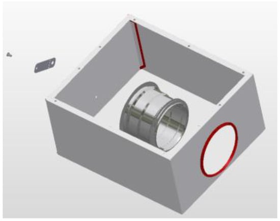
Figure 1.
3D view of a throttle valve.
Currently, the production of TV160 throttle valves takes place on a non-automated production line with Welding, Assembly1, and Assembly2 workstations. One worker works at each workstation of the production line, i.e., there are three in total. The sequence of production operations and their durations according to individual workplaces on the production line are recorded in Table 1. Between the workplaces, there are Buffer1 and Buffer2 interoperation warehouses with a capacity of 10 units, which serve to dampen fluctuations in the line’s activity. At the end of the line there is Buffer3, where the completed production is collected.

Table 1.
The current state of production of TV160—workplaces, production operations, and operating times.
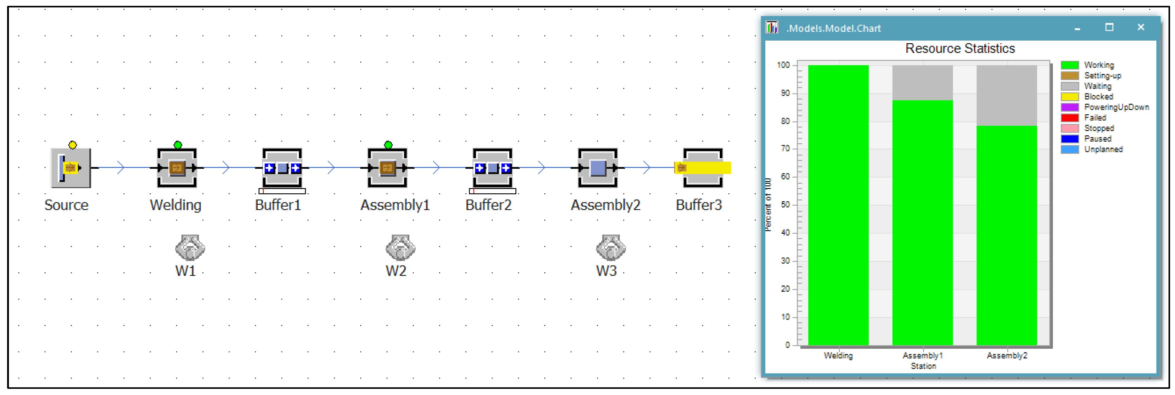
The TV160 production process was recorded using the Tecnomatix Plant Simulation program, as shown in Figure 2, including a graph of the utilization of individual workplaces. The simulation time is eight hours, i.e., one work shift.
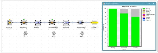
Figure 2.
Current line state.
Based on the facts mentioned above, it can be concluded that 208 TV160 products are produced on the given production line in one eight-hour work shift. This means the hourly production of the line is 26 pieces. It can be concluded that the line is relatively well-balanced, and the workplaces of the line are utilized 80–100%. The bottleneck is the Welding workplace, where the total operating time is 138 s. Interoperation warehouses sized for ten pieces are practically unused, and no stocks larger than one piece are created.
2.2. Methodical Procedure of Solution
The problem in the production of throttle valves is the long-term failure to achieve the planned production, i.e., the inability of the company to meet demand in full. Eliminating this problem is possible by investing in the automation of selected production operations. The introduction of automation into production stabilizes and increases product quality, improves the organization and management of production, humanizes human work, and saves resources. Thus, automation enables the saving of materials, reducing of rejects, reducing of the consumption of technological substances, etc. In addition to the benefits resulting from production cost savings, automation also has secondary effects. These include labor reduction in production preparation and in operative production planning and shortening of the production time of products.
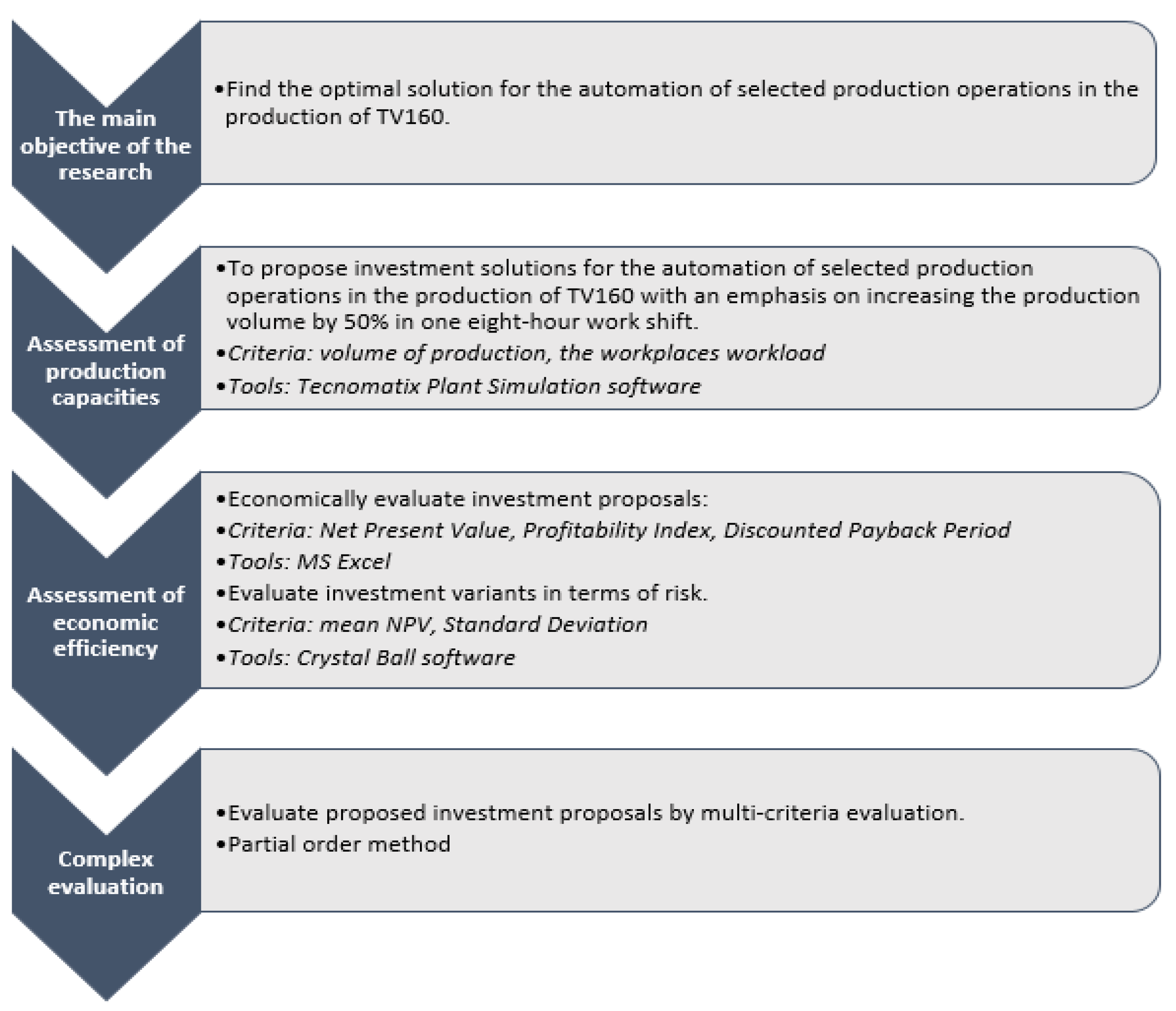
The procedure for solving the problem is documented in Figure 3 and defined in more detail in the following text.
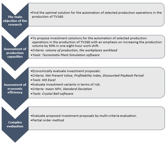
Figure 3.
Procedure for defined problem solving.
The main goal of the research is to find the optimal solution related to investment in the automation of selected production operations of the line. The intention is to ensure an increase in production volume by at least 50% (from 208 pcs/8 h to at least 312 pcs/8 h) and, at the same time, ensure that the investment is economically efficient, even taking into account the risk. The company is not considering the transition from one-shift to two-shift operations.
Assessment of the production capacities of investment variants. A workplace simulation model was created for each investment variant (V1, V2) to assess production capacities. Subsequently, the production process was simulated. The processing time of individual workplaces was entered based on the sum of the times of operations performed at each workplace (1).
where Tp is cumulative processing time, ti is the operating time of the i-th operation, and n is the number of operations at the workplace.
Individual operation times and the cumulative processing time across every workplace are presented in Table 2. The simulation output is a chart showing the utilization of workplaces in % (work time, waiting, and blocking time). Another output is the production volume produced during the simulation, i.e., in an 8 h shift, obtained from workplace statistics.
Table 2.
Proposed state of production—workplaces, production operations, and total times at workplaces in seconds.
Assessment of the economic efficiency of investment variants, including risk. In the first step, economic efficiency evaluation of the proposed investment variants is carried out based on the incremental method. This means that the expected effects and resources expended due to the automation of selected operations on the production line are expressed as the difference between the expected values when implementing the investment option and the values achieved with current non-automated production. The calculation is carried out in MS Excel using a deterministic financial model. Economic efficiency is assessed using three dynamic financial criteria, namely net present value (NPV), profitability index (PI) and discounted payback period (DPP). The mentioned financial criteria support the same decision when evaluating investment variants—to accept or not to accept an investment variant. Their numerical results are different because each financial criterion assesses the investment variant from a different point of view. NPV expresses the profitability of an investment option in an absolute amount for the entire life of the project. PI monitors the return on one euro of capital expenditure. DPP monitors the liquidity of the investment option, i.e., the time for which it will be repaid. The NPV calculation method is given by relation (2), PI relation (3), and DPP relation (4).
The values of the financial criteria are determined by the increase in annual cash flow (CF) from the investment variants converted to the present value at the discount rate (dr), and the amount of one-time investment costs (IC). N is the period of the economic life of the investment, n are the individual years of the economic life of the investment. The relationship for calculating the annual CF from the operating activity is expressed as follows (5):
where EBITDA is the annual increase in the economic result before interest, taxation, and depreciation, ODP is the annual depreciation, and d is the coefficient of the income tax rate.
EBITDA is influenced by production and sales activities. The calculation method for individual investment variants takes into account the number of robots included in the production line, the number of production workers involved in the production process, the annual production volume of the TV160, and more. The calculation of the EBITDA indicator, specifically its annual increase, is expressed by relation (6):
where c is the price per unit of production, Q is the increase in annual production volume, NFIX is the annual increase in fixed costs, and NVAR is the annual increase in variable costs. The annual increase in fixed costs includes the increase in annual depreciation and the increase in annual costs for voluntary insurance of production equipment. The annual increment of variable costs is the sum of the annual increments of direct material consumption, auxiliary material consumption, personnel costs, robot spare parts costs, robot repair and maintenance costs, and other variable costs.
The second step of economic efficiency evaluation considers risk in the proposed investment variants assessment. This is a stochastic approach. Risk consideration will be done using the Monte Carlo method in the Crystal Ball software product. In this step, it is necessary to transform the deterministic financial model into a stochastic one. It is necessary to determine input risk factors and their probability distributions, establish statistical dependencies between the selected risk factors, and define the probability distribution of the output variable (for the selected financial criterion). The simulation process itself is defined by the number of simulation steps, and it is true that the higher the number of repetitions, the higher the accuracy of the results. The simulation results refer to the output variable, which will be the mean value of the financial criterion NPV. The simulation results are generated in numerical form, in the form of statistical characteristics, and in graphical form as a histogram, trend chart, sensitivity chart, overlay chart, and others.
Complex evaluation of the investment variants. It is advisable to choose the optimal version of the investment variant using a multi-criteria evaluation using the partial ranking method. The method is based on determining the sum of the partial order of the production and financial criteria for the compared versions of the investment variants. Partial orders depend on the desired tendency of the criterion value. If the value is descending (for example, DPP), then the criterion with the lowest value will come first. If, on the other hand, the value of the criterion is to increase (for example, NPV), the highest value of the criterion is best-placed. The most advantageous variant is the one whose sum of partial orders is the lowest.
3. Results and Discussion
3.1. Proposals for Investment Variants of Production Line Automation
Achieving the research goal, i.e., increasing the production volume by at least 50% in the production of TV160, is possible only in the production operations of welding and sealing. For this reason, modification of the current TV160 production process is necessary. The Welding workplace will be abolished, and two new workplaces will be created, namely the Pre-assembly workplace and the Robot workplace. At the Pre-assembly workplace, the operations of placing the chimney and placing it in the fixture will take place. The sidewall riveting operation, which took place at the Welding workplace, has been cancelled. The Robot workplace will replace the welding performed at the workplace Welding and the sealing of the chimney performed at the Assembly1 workplace.
Two investment variants for the automated production line (for one and two robots) are proposed in two versions according to the number of workers (three and four). The automation of the production process is ensured at the Robot workplace. Workplaces Assembly1 and Assembly2 do not change. That means the automated production line consists of four workplaces: Pre-assembly, Robot, Assembly1, and Assembly2. The sequence of operations performed at the listed workplaces, including their operating times, is presented in Table 2.
The determination of times for welding and sealing operations performed at the Robot workplace is based on the input data listed in Table 3. The time of the welding operation is the product of the number of welds and the welding time of one weld. The distance between the two welds is set at 77 mm. The time of the sealing operation is determined by the length of the sealant used and the time required to apply it per unit length.
Table 3.
Input data for the calculation of times for welding and sealing operations at the Robot workplace.
Individual investment variants are simulated in the Tecnomatix Plant Simulation software. The simulation output is a chart showing in percentages the time utilization of workplaces, in terms of work time, waiting time, and blocking time. Another output is the volume produced during the simulation, i.e., in 8 h, obtained from workplace statistics. The description of individual investment variants is given in the following text.
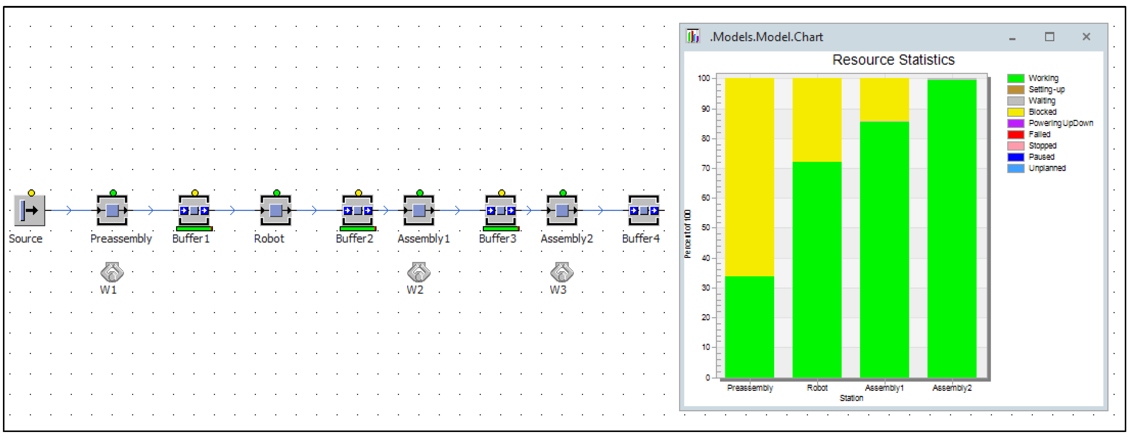
Variant 1a (V1a). In investment variant 1 (Figure 4), the Robot workplace consists of one robot performing both welding and sealing operations. One worker works at the line workplaces Pre-assembly, Assembly1, and Assembly2, so there are three in total. The usability of the robotic workplace is 72%, and the workplace is blocked (fully occupied but not processing) for 28% of the available working time. The bottleneck is the Assembly2 workplace. Low utilization is found at the Pre-assembly workplace, which is only 34% utilized. The production of the line is 292 pcs/8 h, which does not meet the requirement for a 50% increase in the line production capacity.
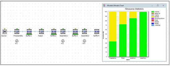
Figure 4.
Variant 1a (one robot, three people).
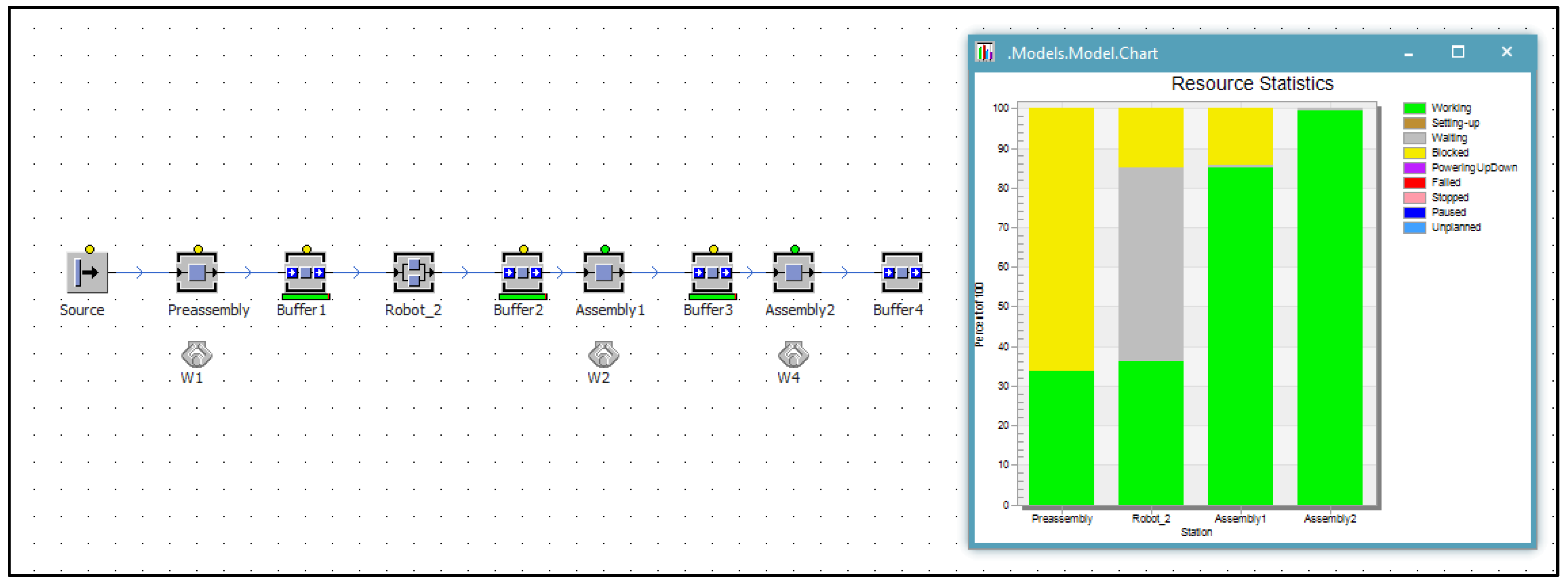
Variant 1b (V1b). In investment variant V1b, the welding and sealing operation is performed by a single robot in the robotic workplace. There are four workers on the line. By adding a fourth worker who works at the Assembly1 and Assembly2 workplaces (in the simulation, a 50%/50% work distribution is considered), the bottleneck of the line will be moved to the robotic workplace (see Figure 5). The utilization of the Assembly workplaces is more than 80%; the Pre-assembly workplace is still only 47% loaded. With the addition of the fourth worker, the line productivity is increased to 434 pcs/8 h, thus meeting the requirement to increase production by at least 50%. In this variant, production will increase by approximately 109%.
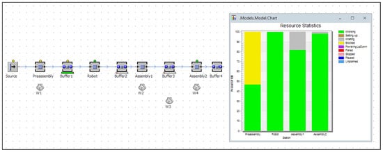
Figure 5.
Variant 1b (one robot, four people).
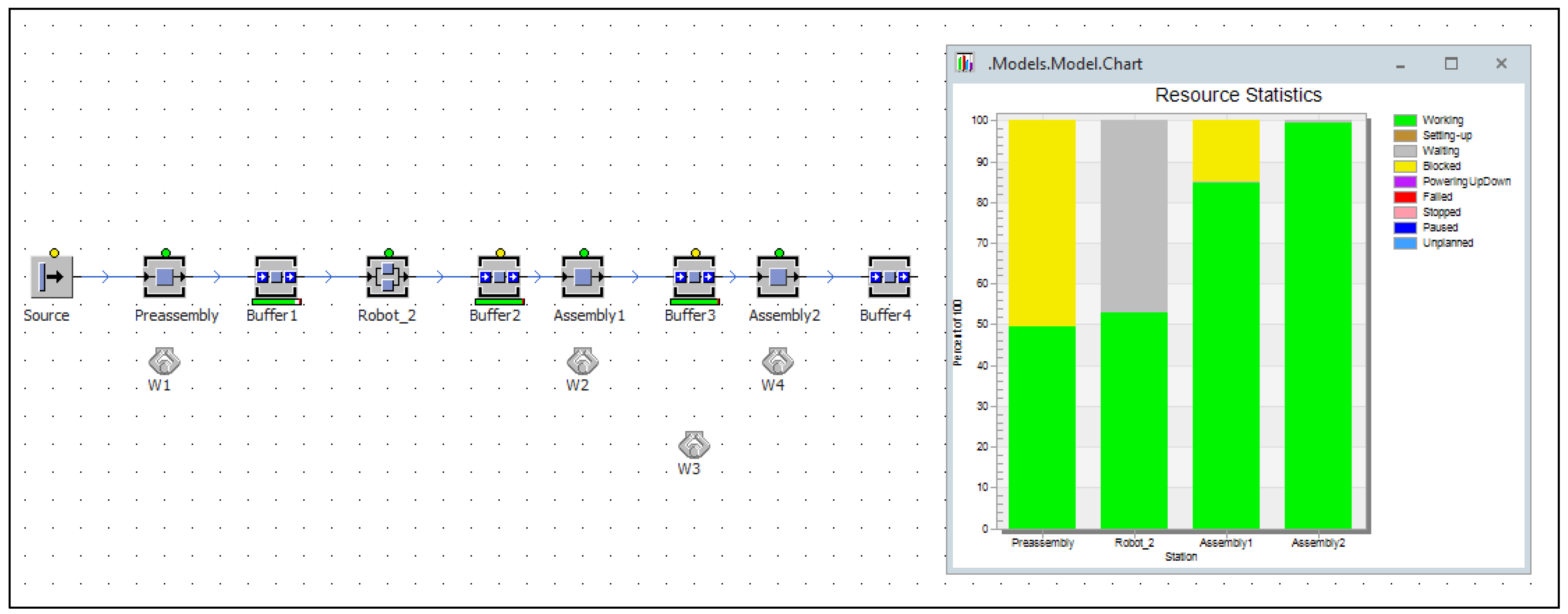
Variant 2a (V2a). In investment variant V2a, there are two robots in a parallel arrangement for welding and sealing operations. Robots perform both operations. There are three workers on the line. The bottleneck is again the Assembly2 workplace (see Figure 6). The line, arranged in this way, can produce 291 pcs/8 h. The utilization of the Assembly1 workplace is more than 80%. The Pre-assembly workplace is only 35% loaded. The parallel robotic workstation is only 36% utilized, 49% waiting, and 15% of the time blocked. In the V2a variant, production will increase by approx. 109% (see Table 4).

Figure 6.
Variant 2a (two robots, three people).
Table 4.
Comparison of the production parameters of the proposed investment variants with the current state.
Variant 2b (V2b). Investment variant V2b has two robots at the Robot workplace connected in parallel (see Figure 7), while both robots perform welding and sealing operations. There are four workers on the production line (one Pre-assembly, one at Assembly1, one at Assembly2, and the fourth worker helps at Assembly1) and two workplaces in a ratio of 50%/50%. The number of robots and the distribution of workers will make it possible to increase the performance of the robotic workplace by 100%, which increases line productivity to 440 pcs/8 h. Workplace utilization is more than 80% in the case of Assembly1. The line bottleneck is Assembly2, whose capacity is fully utilized. The robotic workplace and the Pre-assembly workplace are about 50% utilized. Compared to the current state, production increases by approximately 112%, thus fulfilling the requirement to increase production by at least 50%.
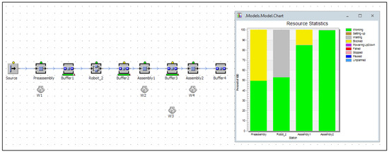
Figure 7.
Variant 2b (two robots, four people).
From the production point of view, it can be concluded that the requirement to increase the production volume by at least 50% was met by investment variants 1b and 2b (see Table 4). Of the listed investment variants, Variant 2b enables the greatest increase in production volume. The production volume of TV160 increases from 207 pcs/8 h (current state) to 440 pcs/8 h, which means an increase of 112.6%.
3.2. Economic Evaluation of Investment Variants of the Production Line
Deterministic approach to evaluating the economic efficiency of investment variants. The company will incur investment costs by procuring robots. Their amount is influenced by the purchase price of the robot/robots and the costs related to their procurement. Selected input data necessary for defining a deterministic financial model and subsequent assessment of the economic efficiency of investment variants are presented in Table 5.
Table 5.
Selected input data for assessing the economic efficiency of investment variants.
When calculating the financial criteria, which are used to assess the economic efficiency of investment proposals, the annual time fund of the robot in the amount of 2014 h is considered. Its utilization is expected to be 85%. Robot, according to Act no. 595/2003 Coll. on income tax, belongs to the second depreciation group with a depreciation period of six years, which is also the lifetime of the investment. Economic calculations consider the price of TV160 at the amount of EUR 9.50 per piece, the hourly labor costs per worker at the amount of EUR 10.50, and the material costs of TV160 at the amount of EUR 10.00 per two pieces.
The resulting values of the financial criteria, according to the proposed investment variants V1, V2 and their versions, are recorded in Table 6. It can be concluded that, from an economic point of view, except for the investment variant V2a, the other proposed versions of the investment variants are acceptable. The best economic results were achieved with version V1b. Its implementation will achieve profitability in the form of monetary income for a period of six years in the amount of EUR 459,578, profitability per one euro of invested investment costs in the amount of EUR 4.31, and a payback period of 1.22 years. The second in line is the investment variant V2b. Marginal economic results are achieved by the investment variant V1a.
Table 6.
Financial criteria of economic efficiency—deterministic approach.
Stochastic approach to evaluating the economic efficiency of investment variants. Taking risk into account in evaluating the economic efficiency of investment variants V1, V2, and their versions is implemented using the Monte Carlo simulation method. Individual input risk factors defined using statistical characteristics and probability distributions are listed in Table 7.
Table 7.
Probability distributions and statistical characteristics of risk factors.
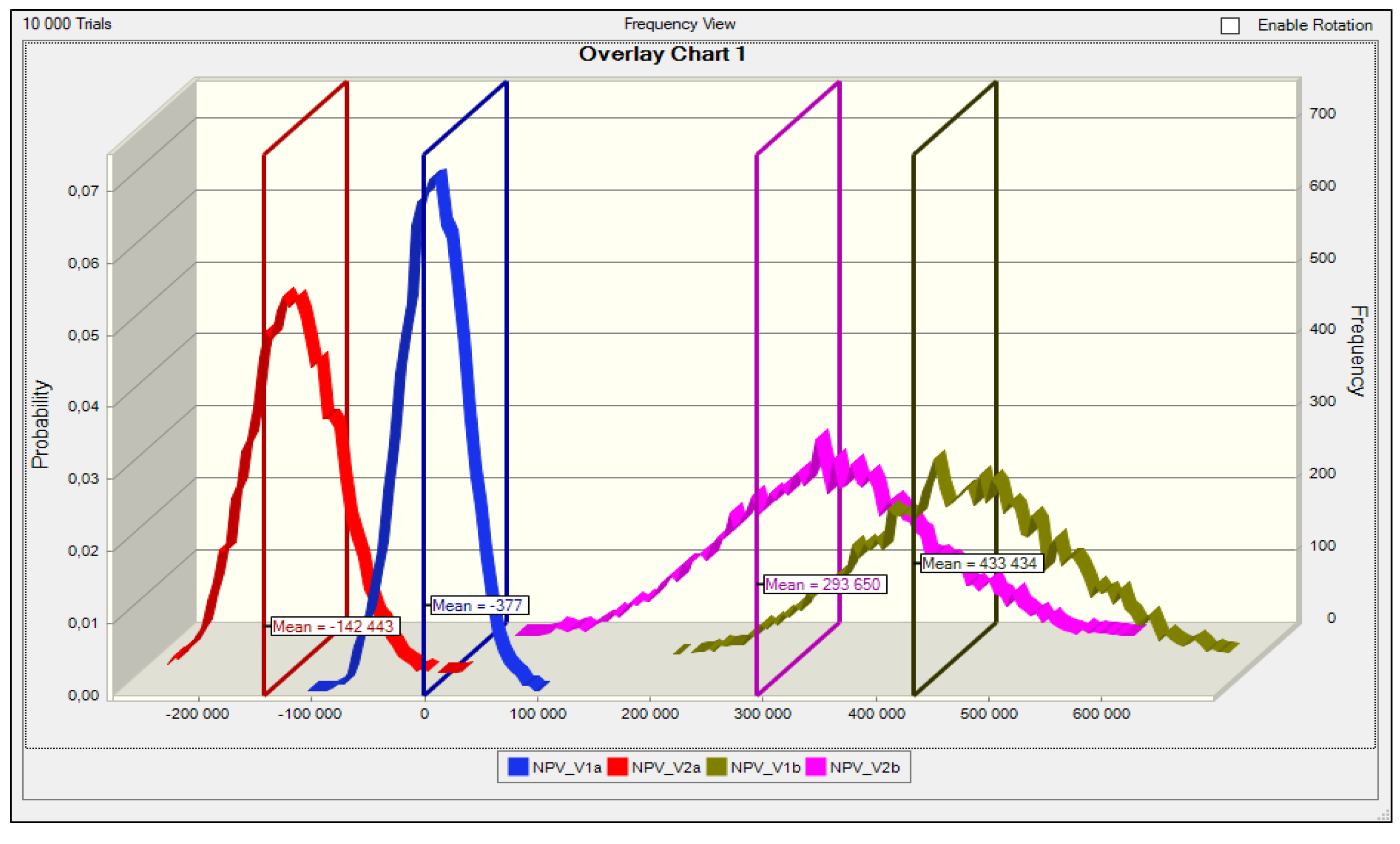
The selection of the most advantageous investment variant, taking into account the risk, is based on the mean value of the financial criterion NPV (mean NPV). The probability distributions of versions of investment variants V1 and V2 are determined by a mix of input risk factors, and their courses are shown in Figure 8. They provide information about the expected value of NPV and the probability of not achieving it or exceeding it.

Figure 8.
Probability distributions of NPV versions of investment variants.
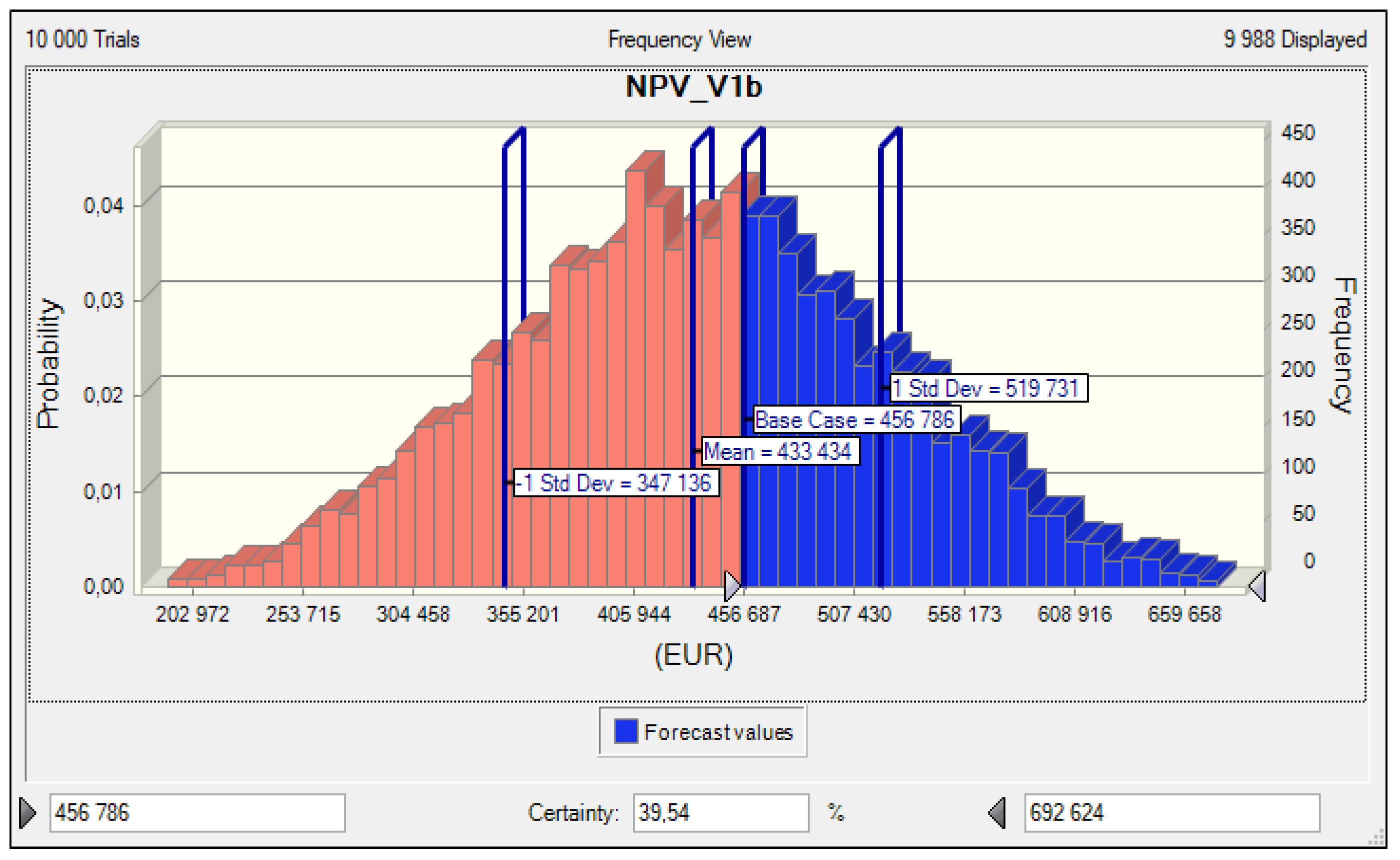
Based on the data presented in Table 8, it can be concluded that the symmetry of probability distributions of NPV is approximately the same for all versions of the investment variants. The NPV probability distributions for all versions are positive, that is, right-skewed, which means that higher values prevail over lower values. Due to the fact that the mean NPVs of the individual versions of the investment variants differ significantly, the rule of mean value and the coefficient of variation are used as decision criteria for determining their advantage. According to the mentioned rule, the version of the investment option that has a higher mean value for the financial criterion and a lower variability is better. The use of this rule confirms that the investment variant version V1b is dominant over the other versions of the investment variants, because it is better in both the considered characteristics compared to them. The NPV_V1b histogram is shown in Figure 9. This documents that, with a probability of 39.54%, higher values of the financial criterion NPV_V1b than in its base case will be achieved.
Table 8.
Selected statistical characteristics of NPV versions of investment variants.

Figure 9.
Probability distribution of NPV_V1b.
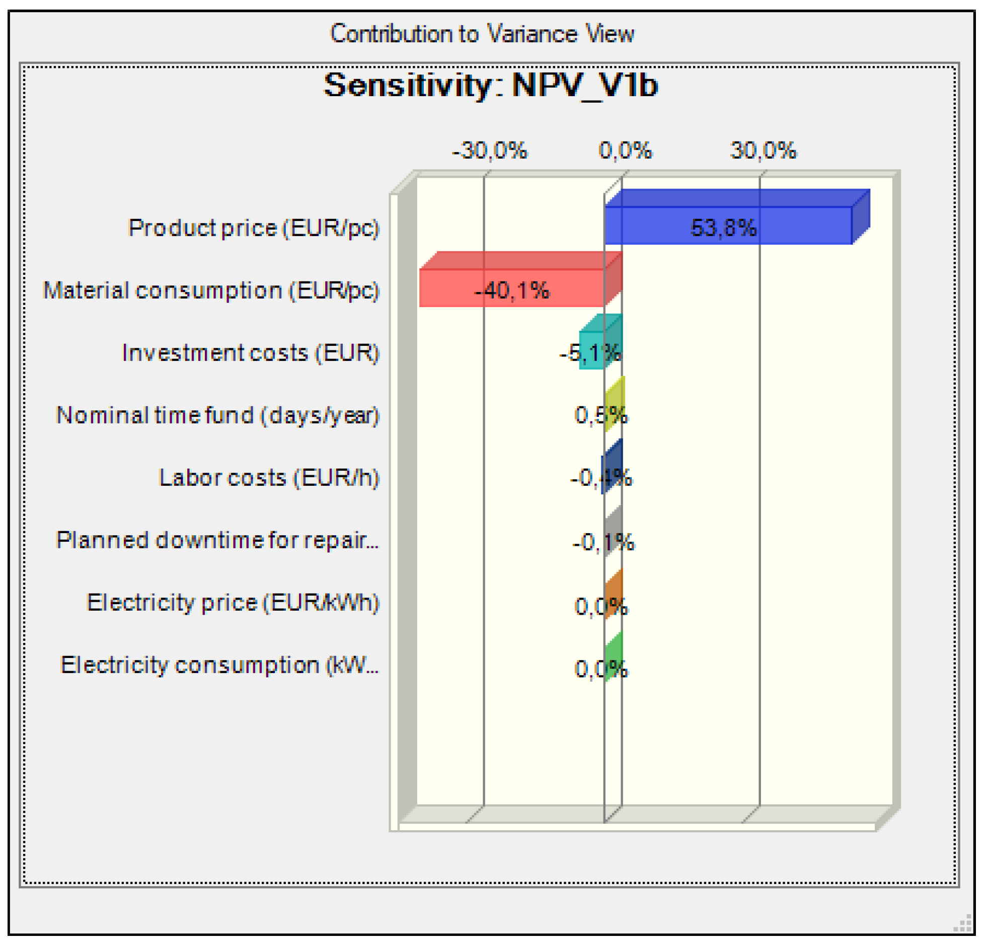
From the sensitivity graph (see Figure 10), it is possible to determine the key risk factors both in terms of the overall forecast uncertainty and their impact on the final value of the financial criterion NPV_V1b. It is clear from the graph that the uncertainty of the NPV_V1b forecast is positively influenced by the price of the TV160 product to the extent of 53.8% and the amount of the nominal time fund to the extent of 0.5%. The uncertainty of the NPV_V1b forecast is negatively affected in the amount of 40.1% by material consumption for the TV160 product, in the amount of 5.1% by the investment costs associated with the procurement of the robot, and in the amount of 0.4% by hourly labor costs.

Figure 10.
Graph of sensitivity of risk factors to NPV_V1b.
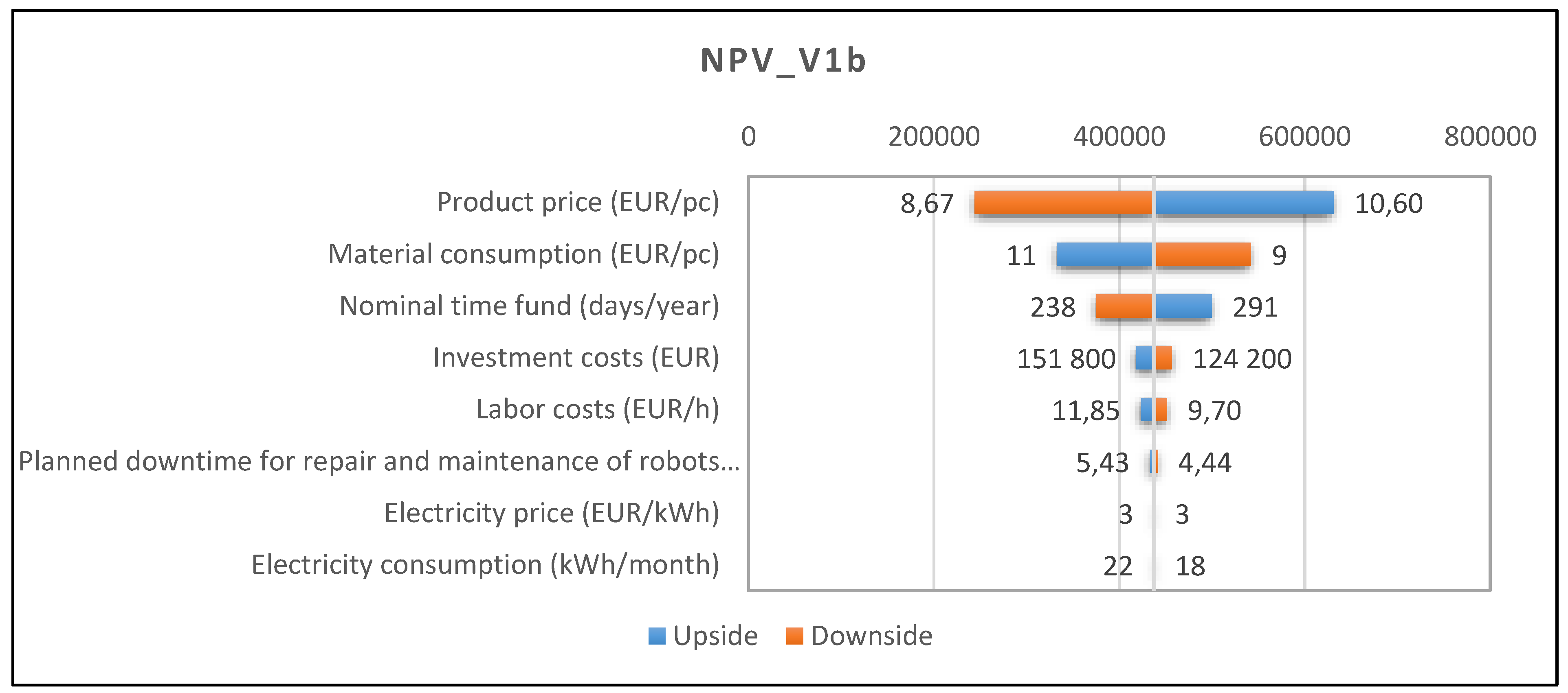
The tornado chart (see Figure 11) shows the strengths of the individual influences of the input variables on the change in the financial criterion NPV_V1b. It shows the variables according to their impact on NPV_V1b for a considered change of ±10%. In the chart, the variables are arranged according to the size of their impact on the financial criterion NPV_V1b. Among the most serious factors causing the NPV_V1b deviation are, in order, product price, material consumption, nominal time fund, investment costs, and labor costs. Less important factors include electricity consumption, electricity price and planned downtime for repair and maintenance of robots.
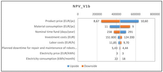
Figure 11.
Tornado chart NPV_V1b.
Due to the effect of taking into account the risk in the most economically advantageous investment variant V1b (see Table 9), there was a decrease in mean NPV_V1b compared to the expected value of NPV_V1b by EUR 23,352, which represents a decrease of 5.1%.
Table 9.
Comparison of NPV_V1b and mean NPV_V1b values.
3.3. Complex Evaluation of Investment Variants
Selection of the optimal version of the investment variant is carried out using a multi-criteria evaluation, using the partial order method. Only those versions of investment variants that meet three conditions are included in the multi-criteria evaluation:
The production condition: i.e., they will ensure an increase in production volume by at least 50%. Only the V1b and V2b versions of the investment variants met this condition.
The condition of economic efficiency, determined by acceptable values of the financial criteria NPV, PI, and DPP. In this case, the condition was met by the versions of investment variants V1a, V1b, and V2b. Version V1a achieves only marginally acceptable values for the financial criteria and at the same time does not meet the production condition; therefore, it is not included in the multi-criteria evaluation.
The condition of economic efficiency, with consideration of risk using the rule of mean NPV and the coefficient of variation. The best values are achieved by the versions of variants V1b and V2b.
The V1b version was determined to be the optimal investment variant based on a multi-criteria evaluation. It achieves the best economic parameters through dynamic financial criteria. In terms of production parameters, it allows one robot to achieve almost identical production volume values as with the V2b version with two robots.
Case studies that have presented the optimization of production processes, either using simulation tools or not, were mentioned in the introduction. This was mainly one critical assessment focused on the production or economic aspects of the project, which either did not include uncertainty in the assessment or only in connection with the economics assessment. In the presented study, the production, finances, and risk aspects are in a complex multi-criteria evaluation (Table 10). However, other authors of scientific papers also point to the need for risk integration in multi-criteria evaluation, albeit in different contexts. For example, the authors of [36] presented a fuzzy multi-criteria decision approach in the selection of a sustainable risk management strategy. Similarly, [37] used a multi-criteria assessment system when choosing the method of operational risk management, and [38] performed a multi-criterion analysis based on integrated process-risk optimization.
Table 10.
Selection of the optimal version of the investment variant by the method of partial orders.
4. Conclusions
Automation of production cannot be done without investment in new equipment or technologies. Although these will expand production possibilities and improve the quality of production operations, on the other hand, they require significant financial resources and imply new risks. A decision on the optimal investment variant is based on an assessment of the investment from several sides. Computer simulation programs are also a supporting tool in decision-making, the potential of which is very large at the moment.
In this article, a comprehensive approach to investment decision-making using simulations was presented through a case study of automation of the production line workplace. Two variants of the investment were proposed according to the equipment of the workplace, with one or two robots, and for each variant two versions of the line service (with three or four workers) were evaluated. Tecnomatix Plant Simulation was used to assess the line in terms of production capacity. The capacity of the line, the bottleneck, and the workload of the workplaces were checked on the simulation models for the individual investment variants. The Crystal Ball program was used for the economic assessment of the investment, including risk factors, where the economic efficiency of the investment was evaluated and risk factors were analyzed using Monte Carlo simulations. The investment variants were assessed first from the point of view of production, where the goal was to achieve production 50% higher than current production. Subsequently, they were evaluated from an economic point of view through the financial indicators of NPV, PI, and DPP. From the point of view of risk, the statistical indicators mean value, standard deviation, and coefficient of variation were selected. The outputs from the individual phases of the investment assessment were ultimately evaluated as a whole by a multi-criteria assessment of the investment variants using the method of partial order.
The primary contribution of the paper is the application of a complex approach to the design of production systems using simulations. However, simulation programs, as a progressive tool in decision-making, were applied only to a limited extent, which is considered a limit of the present research. Their possibilities are much broader, including, e.g., analysis and optimization of all production logistics processes, including interoperation storage and transport. In the case of Monte Carlo simulations, which are part of the Crystal Ball program, it is also appropriate to use the OptQuest module to optimize the process while taking risk into account. A broader application of simulation tools is the intention of future research in this issue.
Author Contributions
Conceptualization, J.J. and J.F.; methodology, J.F. and J.J.; validation, J.J., J.F. and J.K.; formal analysis, J.J., J.F. and J.K.; investigation, J.J. and J.F.; resources, J.F. and J.J.; writing—original draft preparation, J.J., J.F. and J.K.; writing—review and editing, J.F., J.J. and J.K. All authors have read and agreed to the published version of the manuscript.
Funding
This research received no external funding.
Data Availability Statement
Data sharing is not applicable to this article.
Acknowledgments
This paper was developed within the project implementations VEGA 1/0340/21 “The impact of a pandemic and the subsequent economic crisis on the development of digitization of enterprises and society in Slovakia”, VEGA 1/0600/20 “Design of a digital twin for the research of selected operational indicators of hose conveyors in accordance with cleaner production using experimental measurements and simulation approaches”, VEGA 1/0638/19 “Research into the possibilities of designing continuous intra-company transport systems with the support of experimental methods and virtual reality tools”, and KEGA 005TUKE-4/2022 “Increasing the efficiency and quality of the educational process at universities through professional simulators in face-to-face and distance learning and for the needs of dual education”. This work was supported by the Slovak Research and Development Agency under Contract nos. APVV-19-0418 “Intelligent solutions to enhance business innovation capability in the process of transforming them into smart businesses” and APVV-21-0195 “Research of the possibility of digital transformation of continuous transport systems”. This paper was created by the implementation of the project “New possibilities and optimization approaches within logistics processes”, based on the support of the operational program Integrated Infrastructure with ITMS code 313011T567.
Conflicts of Interest
The authors declare no conflict of interest.
References
- Freiberg, F.; Scholz, P. Evaluation of Investment in Modern Manufacturing Equipment Using Discrete Event Simulation. Procedia Econ. Financ. 2015, 34, 217–224. [Google Scholar]
- Aguilar, H.; García-Villoria, A.; Pastor, R. A survey of the parallel assembly lines balancing problem. Comput. Oper. Res. 2020, 124, 105061. [Google Scholar] [CrossRef]
- Van Hop, N. A heuristic solution for fuzzy mixed-model line balancing problem. Eur. J. Oper. Res. 2006, 168, 798–810. [Google Scholar]
- Lin, Y.-C.; Yeh, C.-C.; Chen, W.-H.; Hsu, K.-Y. Implementation Criteria for Intelligent Systems in Motor Production Line Process Management. Processes 2020, 8, 537. [Google Scholar]
- Zhao, R.; Zou, G.; Su, Q.; Zou, S.; Deng, W.; Yu, A.; Zhang, H. Digital Twins-Based Production Line Design and Simulation Optimization of Large-Scale Mobile Phone Assembly Workshop. Machines 2022, 10, 367. [Google Scholar] [CrossRef]
- Daneshjo, N.; Malega, P. Improvement project of production line using automation. TEM J. 2020, 9, 1003–1010. [Google Scholar] [CrossRef]
- Takai, S. An approach to integrate product and process design using augmented liaison diagram, assembly sequencing, and assembly line balancing. J. Mech. Des. Trans. 2021, 143, 1–17. [Google Scholar] [CrossRef]
- Lu, C.; Yang, Z. Integrated assembly sequence planning and assembly line balancing with ant colony optimization approach. Int. J. Adv. Manuf. Technol. 2015, 83, 243–256. [Google Scholar]
- Liu, X.; Yang, X.; Lei, M. Optimisation of mixed-model assembly line balancing problem under uncertain demand. J. Manuf. Syst. 2021, 59, 214–227. [Google Scholar]
- Kalayci, C.B.; Hancilar, A.; Gungor, A.; Gupta, S.M. Multi-objective fuzzy disassembly line balancing using a hybrid discrete artificial bee colony algorithm. J. Manuf. Syst. 2015, 37, 672–682. [Google Scholar] [CrossRef]
- Yilmaz, H.; Yilmaz, M. A multi-manned assembly line balancing problem with classified teams: A new approach. Assem. Autom. 2016, 36, 51–59. [Google Scholar] [CrossRef]
- Hu, X.; Wu, C. Workload smoothing in two-sided assembly lines. Assem. Autom. 2018, 38, 51–56. [Google Scholar] [CrossRef]
- Niroomand, S.; Vizvari, B. Straight assembly line balancing by workload smoothing: New results. IMA J. Manag. Math. 2022, 1–26. [Google Scholar] [CrossRef]
- Fathi, M.; Fontes, D.B.; Urenda Moris, M.; Ghobakhloo, M. Assembly line balancing problem: A comparative evaluation of heuristics and a computational assessment of objectives. J. Model Manag. 2018, 13, 455–474. [Google Scholar] [CrossRef]
- Azizoğlu, M.; İmat, S. Workload smoothing in simple assembly line balancing. Comput. Oper. Res. 2018, 89, 51–57. [Google Scholar]
- Chai, J.-F.; Hu, X.-M.; Qu, H.-W.; Li, M.-H.; Xu, H.-J.; Liu, Y.; Yu, T. Production line 3D visualization monitoring system design based on OpenGL. Adv. Manuf. 2018, 6, 126–135. [Google Scholar]
- Kayar, M.; Akalin, M. Comparing Heuristic and Simulation Methods Applied to the Apparel Assembly Line Balancing Problem. Fibres Text East Eur. 2016, 24, 131–137. [Google Scholar]
- Wang, Y.; Yang, O. Research on industrial assembly line balancing optimization based on genetic algorithm and witness simulation. Int. J. Simul. Model 2017, 16, 334–342. [Google Scholar] [CrossRef]
- Bongomin, O.; Mwasiagi, J.I.; Nganyi, E.O.; Nibikora, I. A complex garment assembly line balancing using simulation-based optimization. Eng. Rep. 2020, 2, e12258. [Google Scholar]
- Mihály, Z.; Lelkes, Z. Improving Flow Lines by Unbalancing. Informatica 2019, 43, 39–44. [Google Scholar] [CrossRef]
- Yang, B.; Chen, W.; Lin, C. The algorithm and simulation of multi-objective sequence and balancing problem for mixed mode assembly line. Int. J. Simul. Model 2017, 16, 357–367. [Google Scholar]
- Song, L.; Jin, S.; Tang, P. Simulation and optimization of logistics distribution for an engine production line. J. Ind. Eng. Manag. 2016, 9, 59–72. [Google Scholar]
- Longo, C.S.; Fantuzzi, C. Simulation and optimization of industrial production lines. At-Automatisierungstechnik 2018, 66, 320–330. [Google Scholar] [CrossRef]
- Pekarcikova, M.; Trebuna, P.; Kliment, M.; Dic, M. Solution of Bottlenecks in the Logistics Flow by Applying the Kanban Module in the Tecnomatix Plant Simulation Software. Sustainability 2021, 13, 7989. [Google Scholar]
- Malega, P.; Gazda, V.; Rudy, V. Optimization of production system in plant simulation. Simulation 2021, 98, 295–306. [Google Scholar]
- Sujová, E.; Vysloužilová, D.; Čierna, H.; Bambura, R. Simulation Models of Production Plants as a Tool for Implementation of the Digital Twin Concept into Production. Manuf. Technol. 2020, 20, 527–533. [Google Scholar] [CrossRef]
- Grabowik, C.; Ćwikła, G.; Kalinowski, K.; Kuc, M. A Comparison Analysis of the Computer Simulation Results of a Real Production System: Production System Modelling with FlexSim and Plant Simulation Software. Adv. Intell. Syst. Comput. 2020, 950, 344–354. [Google Scholar]
- Suhanyiova, A.; Suhanyi, L. Analysis of depreciation of intangible and tangible fixed assets and the impact of depreciation on the profit or loss and on the tax base of the enterprise. In Proceedings of the 18th International Scientific Conference on International Relations—Current Issues of World Economy and Politics, Smolenice, Slovakia, 30 November–1 December 2017; pp. 939–950. [Google Scholar]
- Zhao, J. Risk Assessment Method of Agricultural Management Investment Based on Genetic Neural Network. Secur. Commun. Networks 2022, 2022, 1–10. [Google Scholar] [CrossRef]
- Ilbahar, E.; Kahraman, C.; Cebi, S. Risk assessment of renewable energy investments: A modified failure mode and effect analysis based on prospect theory and intuitionistic fuzzy AHP. Energy 2022, 239, 121907. [Google Scholar]
- Khalfi, L.; Ourbih-Tari, M. Stochastic risk analysis in Monte Carlo simulation: A case study. Commun. Stat. Simul. Comput. 2019, 49, 3041–3053. [Google Scholar]
- Huo, Y.; Xu, C.; Shiina, T. Period value at risk and its estimation by Monte Carlo simulation. Appl. Econ. Lett. 2021, 29, 1675–1679. [Google Scholar] [CrossRef]
- Tobisova, A.; Senova, A.; Rozenberg, R. Model for Sustainable Financial Planning and Investment Financing Using Monte Carlo Method. Sustainability 2022, 14, 8785. [Google Scholar]
- Abba, Z.Y.I.; Balta-Ozkan, N.; Hart, P. A holistic risk management framework for renewable energy investments. Renew Sustain. Energy Rev. 2022, 160, 112305. [Google Scholar]
- Zhu, L. A simulation based real options approach for the investment evaluation of nuclear power. Comput. Ind. Eng. 2012, 63, 585–593. [Google Scholar] [CrossRef]
- Edjossan-Sossou, A.M.; Galvez, D.; Deck, O.; Al Heib, M.; Verdel, T.; Dupont, L.; Chery, O.; Camargo, M.; Morel, L. Sustainable risk management strategy selection using a fuzzy multi-criteria decision approach. Int. J. Disaster Risk Reduct. 2020, 45, 101474. [Google Scholar] [CrossRef]
- Ristanović, V.; Primorac, D.; Kozina, G. Operational Risk Management Using Multi-Criteria Assessment (AHP Model). The. Vjesn. 2021, 28, 678–683. [Google Scholar]
- Derradji, R.; Hamzi, R. Multi-criterion analysis based on integrated process-risk optimization. J. Eng. Des. Technol. 2020, 18, 1015–1035. [Google Scholar]


Disclaimer/Publisher’s Note: The statements, opinions and data contained in all publications are solely those of the individual author(s) and contributor(s) and not of MDPI and/or the editor(s). MDPI and/or the editor(s) disclaim responsibility for any injury to people or property resulting from any ideas, methods, instructions or products referred to in the content. |
© 2023 by the authors. Licensee MDPI, Basel, Switzerland. This article is an open access article distributed under the terms and conditions of the Creative Commons Attribution (CC BY) license (https://creativecommons.org/licenses/by/4.0/).