Article

Simulation Prediction and Experiment of Brittle Damage of Cemented Carbide Microgroove Turning Tools Based on Peridynamics

1
School of Mechanical Engineering, Guizhou Institute of Technology, Guiyang 550003, China
2
School of Mechanical Engineering, Guizhou University, Guiyang 550025, China
*
Author to whom correspondence should be addressed.
Processes 2023, 11(2), 520; https://doi.org/10.3390/pr11020520
Submission received: 6 January 2023 / Revised: 27 January 2023 / Accepted: 3 February 2023 / Published: 8 February 2023

Abstract

:
Brittle damage is a key factor restricting tool life extension. The peridynamic (PD) theory was applied to explain and predict the brittle damage of the near-field of the cutting edge of a cemented carbide microgroove turning tool (CCMTT) for the first time in this study, and the PD modeling of the complex surface was realized. The results showed that the PD modeling accuracy of the CCMTT can reach ± 3.4 % . The displacement of material points in the near-field of the cutting edge of the CCMTT is caused by the combined effect of the external load and the internal interaction force, and the former is dominant. There is no linear relationship between the displacement and the calculation time; instead, there are fluctuations and a maximum increase in the material point displacement in the main cutting direction. Only microdisplacements of material points in the near-field of the cutting edge occur under the given cutting conditions. The accumulation of microcracks caused by microdisplacement does not reach the transition threshold to form macrocracks. This agrees well with the experimental results, and the relative error can be controlled within 3.2%.

1. Introduction

The brittle damage of cemented carbide tools is an important failure mode, which is the process of the tool material changing from a continuum to a non-continuum. Therefore, we also call it “discontinuous breakage”. Tools are easily damaged (broken) due to the impact load in the metal-cutting process. In particular, brittle damage can become more serious when a tool with greater brittleness, such as a cemented carbide tool, is used to machine intermittently or to process high-hardness materials. Many researchers have focused on tool damage recognition and monitoring in the cutting process and solved tool damage using cutting experiments. Qian et al. [1] studied the relationship between tool damage and working conditions and established a correlation model. A novel method for detecting tool damage automatically on CNC machines in real time was presented by Cho et al. [2] and was used to detect the fractured state of tools using the signals of CNC spindle motor loads. Buchkremer et al. [3] proposed a new non-iterative calibration procedure, which described the relationships between tool damage and thermomechanical state variables of the chip-free surface, to realize the monitoring of tool damage. Tool damage was also detected using a machine vision approach during the turning of hardened steel in research by Lee et al. [4]. Meanwhile, many scholars have studied the mechanism of tool damage using cutting experiments aimed at tool damage, which is the most typical method in the traditional research of tool damage. Mohamed et al. [5] and Ma et al. [6] focused on the problem of tool damage during the cutting process through cutting experiments, scanning electron microscopy (SEM), energy-dispersive spectroscopy (EDS) and X-ray photoelectron spectroscopy (XPS) and found that the tool damage experienced three stages: microcrack generation, microcrack propagation and brittle fracture. The bond breakage of carbide turning tools was also analyzed using the finite element method and cutting experimental method [7]. Cheng et al. [8], Kresse et al. [9] and Cui et al. [10] all discussed the breakage behavior of cutting tools during the milling or turning process through experiments. All of the research above is about tool damage solved using traditional cutting experiments and is based on the real occurrence of tool damage.
Microcracking is the only mode of brittle damage in various cutting tools, such as breakage, edge collapse, spalling and macrocracking. Their differences mainly lie in the crack size, shape, initiation and propagation time [11,12]. The common feature is the transformation of materials from continuity to discontinuity. Traditional research methods, such as online monitoring and identification, cutting tests and finite element analysis, are limited by the hypothesis of the spatial continuity of research objects. The peridynamic (PD) theory has unique advantages in solving discontinuous damage and has developed rapidly, to some extent, as a new theory. The basic peridynamic theory was put forward by Dr. Silling [13] of Sandia National Laboratory in 2000. Based on the idea of nonlocal action, the theory has a unified expression for mechanical behavior from continuous to discontinuous and from microscopic to macroscopic. The efficacy and computational cost of peridynamic surface correction methods for elasticity and fracture were investigated by Le et al. [14], and practical suggestions for reducing the peridynamic surface effect were provided. Liu et al. [15] presented a combined peridynamic nonlocal and classical local damage model for failure prediction to effectively model the spontaneous shear-band-to-crack switching phenomenon. An elastoplastic model based on an ordinary state-based peridynamic theory and a plastic flow rule based on the yield function were established by Pashazad et al. [16], and the numerical results showed that the proposed PD elastoplastic model could predict plastic yielding. An effective and accurate way to couple FEM meshes to peridynamic grids was proposed by Zaccariotto et al. [17], and it is used to solve crack propagation with crack-branching problems. The combination of classical and peridynamic theories from Jafari et al. [18], a novel 3D conjugated bond-pair-based peridynamic model to simulate the initiation and propagation of cracks in brittle solids from Wang et al. [19], a peridynamic model for polycrystalline AlON to investigate the failure evolution observed in experiments from Zhang et al. [20], pure basic theoretical studies of peridynamics, such as fracture pathways, multi-scale grid models, bond and state basis, dissipation equations, and local and nonlocal mixed models from Alali et al. [21], an original full orthotropic model for in-plane linear elasticity based on the peridynamic theory from Diana et al. [22], a radically new strategy to couple grids with different spacing to increase the peridynamic computational efficiency and a new algorithm to solve the cases of crack propagation in brittle materials from Shojaei et al. [23] are all focused on the basic theory of PD and aimed at simple geometrical structures. Silling et al. [24] considered a peridynamic model in a typical particle discretization suffering from zero-energy mode instability and added a term to the corresponding strain energy density that resists deviations from a uniform deformation to eliminate these modes. In addition, many researchers have focused on the experimental study of the brittle damage of materials [25,26,27]. All of the research above demonstrated that the peridynamic (PD) theory has obvious advantages in analyzing discontinuous damage; however, it is only applied to typical brittle materials with simple geometrical structures at present, such as planes, circular holes, and cylindrical surfaces for typical brittle materials such as glass, concrete, cast iron and so on. The application of PD to the calculation of cemented carbides with complex curved surfaces has never been reported because of difficulties in modeling a complex curved surface.
The peridynamic theory was applied to research the brittle damage of the near-field of the cutting edge of a cemented carbide microgroove turning tool (CCMTT) for the first time in this study. The CCMTT is a self-developed turning tool fabricated in previous research and has a curved-surface microgroove on its rake face. The PD numerical analysis method for the brittle damage of the CCMTT was established by building a boundary control mathematical model of the CCMTT. This research will provide a new idea for the mechanical reliability evaluation of cemented carbide turning tools (CCTTs) with complex curved surface microstructures and serve as a reference for the PD micromechanical research on inhomogeneous materials with complex surfaces.

2. Materials and Methods

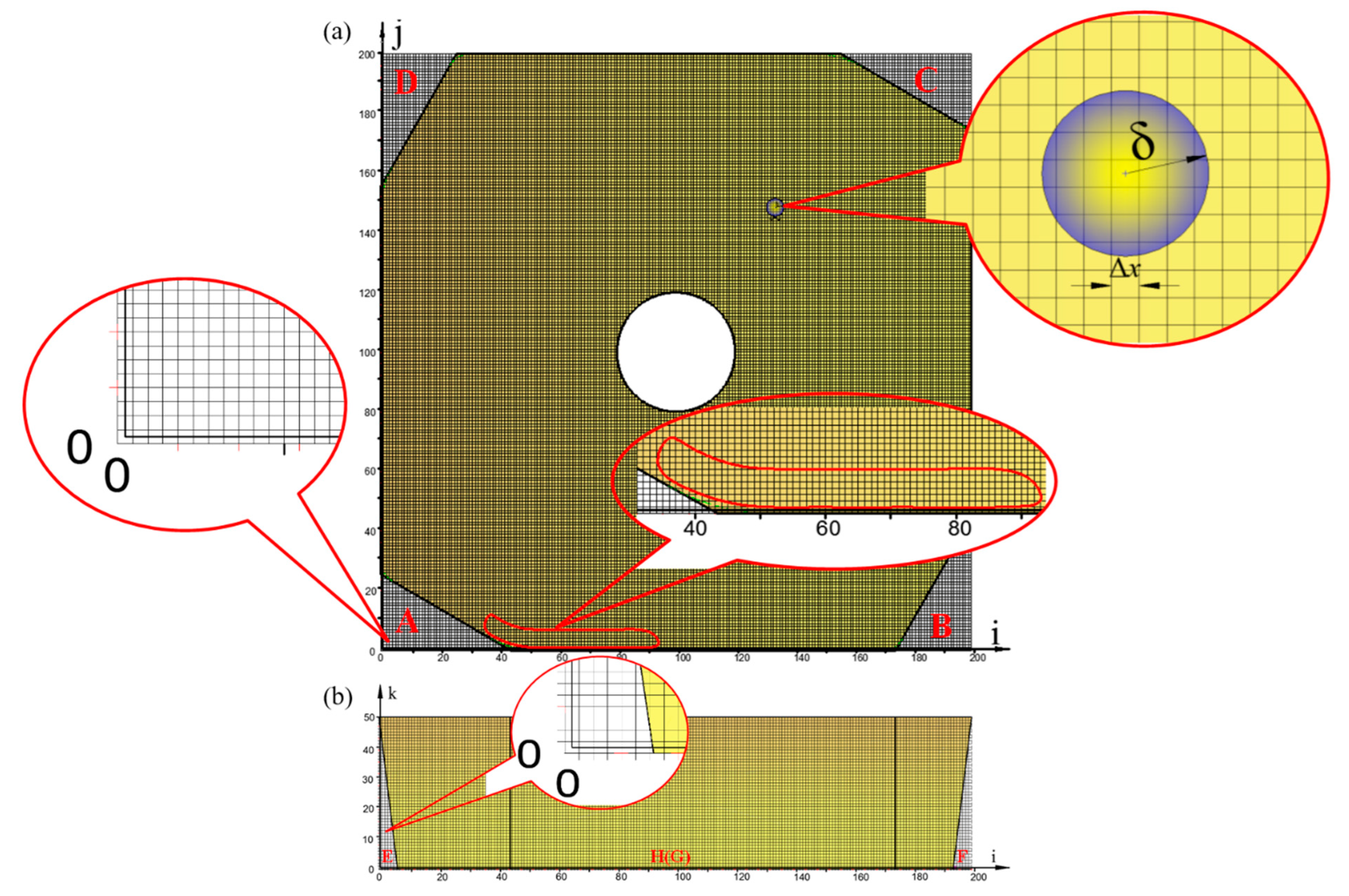
2.1. Establishment of Bond-Based Peridynamic Methods

In space and time, each point in an object represents the position of a material point, and each material point occupies a coordinate x i   i = 1 , 2 , , , a volume V i and a corresponding material density ρ i . Every material point may be changed by the action of physical force, displacement or velocity. In the peridynamic theory, any material point obeys the Lagrange description; that is, in the Cartesian coordinate system, the motion of the object is expressed by describing the spatial position of each material point at different times [28,29,30,31]. Based on the law of universal gravitation, the peridynamic theory can be formed: the motion of each point between any two material points of an object can be described by the interaction force f 0 . If the object is discretized into finite material points, certain interaction forces exist among these points, and when the distance between the two material points is more than a certain length δ , the interaction force f 0 between the two material points is zero [16,32]. According to the peridynamic theory, it is assumed that the object occupies a reference domain R, and any material point i in the reference domain has a reference subdomain R i 0 with a radius of δ , and there is an interaction force f 0 between material point i and any point material point j within the subdomain shown in Figure 1.
According to Newton’s second law, the fundamental peridynamic equation of motion of any point i at time t in the reference domain can be expressed as:
ρ u ¨ x i , t = R i 0 0 f 0 u x j , t u x i , t , x j x i d V j + b x i , t t 0   , j R i 0
In the formula, ρ is the material density, u ¨ is the acceleration of a material point at a certain time, u is the displacement field of a material point, b is the volume force density of the external force, and V i is the volume of material point i [33,34]. The forces acting on any material point i in the reference domain include the internal forces L i from the other material point in subdomain R i 0 acting on material point i and the external forces b i exerted on material point i by the external load:
L i = L x i , t = R i 0 f 0 u x j , t u x i , t , x j x i d V j x R , t 0
  b i = b x i , t
Then, Equation (1) can be simplified to:
ρ u ¨ x i , t = L x i , t + b x i , t t 0   , j R i 0
Material point x i interacts with other material points in subdomain R i 0 , so its motion state is affected by the cumulative deformation of these points and deforms correspondingly. Material point x j will also be affected by the cumulative deformation of the material points in subdomain R j 0 . In order to describe the motion state of the material point more accurately, two physical quantities are introduced here: the relative displacement η between the two material points and the relative position ξ 0 . In the deformation part of the object, the initial relative position vector of material points x i and x j before deformation is ( x j x i ), and after displacements of u i and u j , respectively, the relative position vector of the two material points is changed to ( x j x i ) [35]; then:
η = u j u i = u x j , t u x i , t
ξ 0 = x j x i
It is known from Newton’s third law that the interaction force between any two material points in an object is equal in size and opposite in direction, and the direction of the force is parallel to the connection between the two material points. Then:
f 0 η , ξ 0 = f 0 η , ξ 0   η , ξ 0
After the deformation of the two material points, according to the conservation law of linear momentum, the following equation can be obtained:
f 0 η , ξ 0 × η + ξ 0 = 0   η , ξ 0
So, a general form of the PD force function can be obtained based on Equation (7) and Equation (8):
f 0 η , ξ 0 = F η , ξ 0 × η + ξ 0   η , ξ 0
where F η , ξ 0 is a scalar-valued even function.
In bond-based peridynamics, a material can be called microelastic if it satisfies Equation (10):
η × f 0 η , ξ 0 = 0   ξ 0 0
If the interaction force between material points satisfies Equation (11) in peridynamics, then the object is also a microelastomer:
f 0 η , ξ 0 = w η η , ξ 0
In the formula, w is a scalar potential function, which is the energy of a single bond. For a given material point, its unit volume energy can be expressed as:
w = 1 2 R i 0 0 w η , ξ 0 d V i
The coefficient 1/2 indicates that the vertex of a bond has only half the bond energy. When the object is a linear material, the function of the constitutive force f0 of the object can also be expressed as:
f 0 η , ξ 0 = C ξ 0 · η + f 0 0 , ξ 0   η , ξ 0
In the formula, C is the micromodulus function of the material, which is a second-order tensor and defined as:
C ξ 0 = f 0 η 0 , ξ 0   ξ 0
Taking the partial derivative of Equation (9) with respect to η :
f 0 η η , ξ 0 = ξ 0 · F η η , ξ 0 + F η , ξ 0   η , ξ 0
where is the sign of the dyadic product.
Thus, C ξ 0 can be expressed as follows:
C ξ 0 = ξ 0 · F η 0 , ξ 0 + F 0 , ξ 0   η , ξ 0
Combined with Equation (10), another new result can be obtained:
η × f 0 η , ξ 0 = i j k f 0 η 1 f 0 η 2 f 0 η 3 f 1 f 2 f 3 = f 3 η 2 f 2 η 3 i + f 1 η 3 f 3 η 1 j + f 2 η 1 f 1 η 2 k = 0
which implies:
f i η j = f j η i for   i ,   j = 1 , 2 , 3
The function C ξ 0 also satisfies the property of the even function, that is:
C ξ 0 = C ξ 0   ξ 0
Thus, for a microelastic material, the interaction force between the two material points can be expressed as:
f 0 η , ξ 0 = η + ξ 0 η + ξ 0 · c · s η , ξ 0 · μ t , ξ 0   η , ξ 0
In the formula, c represents the bond stiffness constant, which is related to the bulk modulus E and the radius of the reference domain δ and is defined as:
c = 18 E π δ 4
E = 2 3 E
Among them, E represents the Young modulus of the material.
μ t , ξ 0 is a scalar function that defines the failure condition of a bond, and s represents the elongation of the bond and can be defined as:
s t , η , ξ 0 = η + ξ 0 ξ 0 ξ 0   η , ξ 0
When μ is taken to be 1, it represents a complete bond. When μ is taken to be 0, the elongation of the bond reaches the limit s 0 , and there is no interaction between the material points, and the bond is permanently broken [36,37]. At a certain time t, the damage degree at material point i of the material can be expressed by the proportion φ ( x , t ) of the complete bonds:
φ ( x , t ) = 1 R i 0 μ t , ξ 0 d V i R i 0 d V i
where 0 < φ < 1. When φ   = 0, it indicates the initial state of the material. When φ   = 1, it indicates that all bonds around the material point break. Because the broken bond no longer bears tensile stress, the accumulation and expansion of the broken bond will form a microscopic fracture surface, and the accumulation of the microscopic fracture surface will reach a certain threshold [38]. This will lead to a significant decrease in the limit strain value of the macroscopic object and cause macroscopic damage to the object.
According to the peridynamic theory, by defining the elongation s η , ξ 0 of the bond between material points, according to the critical stretch s 0 of the material, the judgment conditions are established as follows:
μ t , ξ 0 = 1 s η , ξ 0 < s 0 0 s η , ξ 0 s 0
According to the critical stretch s 0 of the material, whether the real-time elongation s η , ξ 0 of the bond between any two material points is greater than or equal to s 0 is determined so as to judge whether bond damage occurs at the material point. The critical stretch s 0 is not a constant but a variable that changes with time, which can be defined as follows:
s 0 t , η , ξ 0 = s 00 α s min t , η , ξ 0
s min t , η , ξ 0 = min s t , η , ξ 0 = min η + ξ 0 ξ 0 ξ 0
in which s 00 is ultimate elongation (a material constant), α is the material safety factor, and s min is the minimum among the elongations of bonds formed by all material points at the moment.
Based on the PD theory, in the process of numerical analysis, the solution to the spatial integral equation is transformed into the solution of the finite sum of the material points [39]. Moreover, we need to consider the interaction between the material points in the reference subdomain δ . There is another material point x j satisfying the inequality x j x i < δ . Equation (1) can be discretized as follows:
ρ u ¨ i x i , t = j f 0 u j n u i n , x j x i · V j + b i n t 0   , j R i 0
In the formula, n indicates the order number of the time step, and V j indicates the volume of material point x j . Δ x is defined as the volume constant of a cubic lattice. Because the reference domain is uniformly dispersed:
V j = Δ x 3
u i n = u x i , t n
In order to reduce the calculation error as much as possible without significantly reducing the calculation efficiency, the volume reduction factor β 0 is introduced to improve the accuracy of the numerical calculation of the volume force. Then:
β 0 = 1 δ + 0.5 Δ x ξ 0 Δ x 0   ξ 0 δ 0.5 Δ x δ 0.5 Δ x < ξ 0 δ + 0.5 Δ x Others
The introduction of the volume reduction factor β 0 changes the volume integral range of the volume force of the material point to be calculated and further reduces the deviation between the theoretical integral volume and the actual integral volume, thus improving the accuracy of the numerical calculation of peridynamics.
It can be seen clearly from Figure 2a,b that the calculation error is closely related to the volume constant of a cubic lattice Δ x ; therefore, an appropriate cubic lattice is favorable to decrease calculation errors.

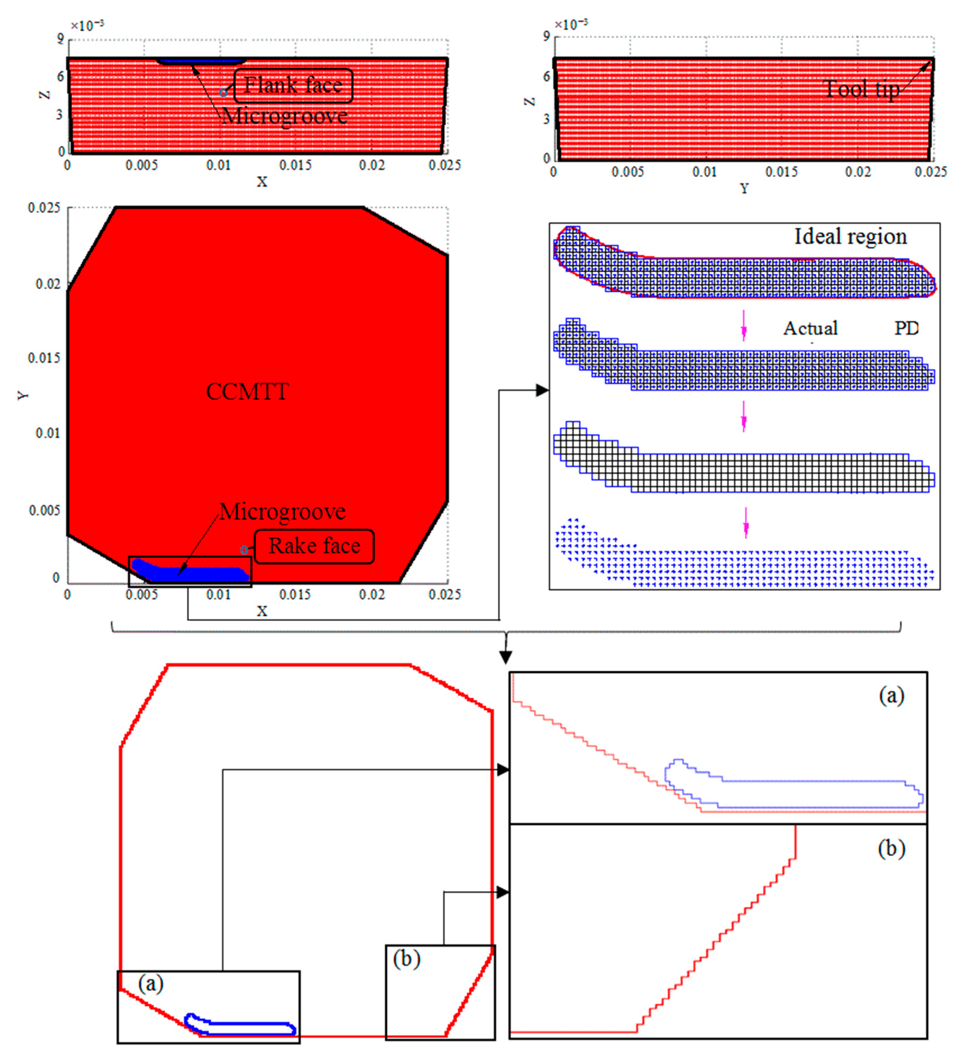
2.2. PD Model of CCMTT

The PD model of the CCMTT established in this paper is based on the integral operation of the basic motion equation of peridynamics. The primary problem to be solved is to effectively express a CCMTT using a finite number of cubic lattices, so the CCMTT is assumed to be represented by a finite number of material points (cubic lattices). However, compared with an ordinary turning tool with a flat rake face, the discretization of the CCMTT is more difficult, and the most typical embodiment is the discretization of the microgroove on the rake face. The size of the microgroove is very small. If the discretization of the microgroove structure is not handled properly, it will cause greater modeling and calculation errors. In addition, the boundary of the microgroove cannot be described by mathematical models because of its irregularity. In order to improve the reproducibility of the microgroove, it is necessary to pay special attention to the selection of material points. Finally, the visualization of the discrete data of the microgroove is another difficulty, and the poor regularity of the microgroove may cause visual distortion.
The 3D geometric model and 2D cutting model (cutting conditions) of the CCMTT are shown in Figure 3, in which Figure 3a is the three-dimensional geometric model of the CCMTT, and the 2D cutting model of the CCMTT, including tool angles, load conditions and their directions, is shown in Figure 3b. The turning tool cuts under the combined action of the main cutting force Fc, the axial thrust force Ff and the radial thrust force Fp, which are measured using a three-dimensional dynamometer, to be described in detail below. The whole cutting process is performed under the cutting conditions v c = 115 m/min, f = 0.42 mm/r (a large feed rate) and a p = 2 mm (a large cutting depth), which are the cutting parameters recommended by the actual production industry. The main tool angles are a large tool tip angle ε r   = 150° and a small main cutting-edge angle k r = 27.5°, and other tool angles are explained below. According to the geometric characteristics and the working conditions of the CCMTT, the PD calculation accuracy and the calculation efficiency were analyzed, and the analysis results are shown in Figure 4.
According to the analysis results shown in Figure 4, the volume constant of the cubic lattice Δx of the PD model of the turning tool is taken to be 0.125 mm, and then Vj = 1.953125 ×   10 3 mm. The radius δ of the reference subdomain of the material point is taken to be 3Δx, i.e., 0.375 mm in the peridynamic numerical analysis. Taking account of the computation accuracy and computation efficiency, the calculating time step dt is taken to be 1 × 10⁻⁹ s, and the solid point is used as the carrier of the physical properties of the tool material, mainly including the volume, mass, density, elastic modulus, fracture limit and so on. In the process of PD analysis, it is necessary to determine the main motion states of all material points under the combined action of the external load and internal interaction force between material points at each time step, including velocity, acceleration, displacement, relative position, relative displacement and so on, so as to calculate the relative displacement between the material point to be solved and the material point applying force and the position of the material point to be solved. In the process of determining the numerical solution of PD, two calculating ranges need to be distinguished: when the calculating time t = 0, the displacement of each material point is in the initial state, and when t ≥ 1, different calculation methods are used. This paper focuses on the boundary control of the microgroove, asymmetrical four-fold edges and symmetrical four-chamfer edges on the rake face of the CCMTT. The PD calculation model of the CCMTT is shown in Figure 5.
Assuming that the location sequence numbers of the material points in the three perpendicular directions of the Cartesian coordinate system are i, j and k, the three-dimensional coordinates of each material point can be expressed as follows:
x i = i · Δ x + Δ x 2
y i = j · Δ x + Δ x 2
z i = k · Δ x + Δ x 2
When the peridynamic calculation time t = 0, according to the location sequence number and the volume constant of the cubic lattice of each material point, the spatial position of all material points representing the whole CCMTT is calculated according to Equations (1)–(34). The center hole of the CCMTT has no effect on the analysis results of the near-field of the cutting edge; therefore, its modeling can be ignored to improve the computational efficiency. Then, the PD model of the CCMTT can be established and presented by a data visualization module of MATLAB, as shown in Figure 6. The PD modeling accuracy of the geometric contour of the CCMTT and the microgroove on the rake face can be controlled within ± 1.5 % and ± 4.9 % , and the modeling accuracy of the whole CCMTT can be controlled within ± 3.4 % .

2.3. Determination of Loaded Area

In order to analyze the motion states of the discrete material points of the CCMTT under the external impact load, the position of the load acting on the turning tool should be determined first. There are different views on the study of the tool–chip action area in the cutting process: point contact theory, line contact theory and surface contact theory. In this research, the CCMTT has a large tool tip angle ( ε r   = 150°), a very small main cutting-edge angle ( k r = 27.5°), a large cutting depth and a large feed rate (vc = 115 m/min, f = 0.42 mm/r, ap = 2 mm, which are the cutting parameters used in the cutting production process), as shown in Figure 3b; the workpiece is difficult-to-machine material with high hardness, and its deformation coefficient is not as large as those of superalloy and titanium alloy. These comprehensive factors determine that the tool–chip contact state is an area contact with a certain length and width, as shown in Figure 7.
According to the discrete processing of the turning tool in the previous paper, the number of material points in the loaded area on the rake face of the CCMTT is calculated, which is defined as p. According to the PD theory, external loads are uniformly applied to each material point in the loaded area. In the cutting process, the impact load applied to the tool has a significant effect on the brittle damage of the CCMTT. The impact loads collected from cutting experiments are taken as the input of the external loads in the PD analysis. The impact loads on the CCMTT are defined as F. The other material points in the unloaded area of the turning tool are not affected by external loads (the value of the external load is 0), and the force on each material point in the loaded area can be expressed as follows:
f i = F p
According to Equation (1) mentioned above and Newton’s second law, the initial acceleration of all material points in the loaded area of the CCMTT can be obtained.
a i = f i ρ V i = f i ρ Δ x 3
Then, the initial velocity and displacement of the corresponding material point can be obtained.
s i = 1 2 a i Δ t 2
v i = a i Δ t
Through the numerical calculation of Equation (32) to Equation (38), the motion states of all material points in the loaded area of the turning tool during the period from the beginning of force application (t = 0) to the end of the first time step, namely, acceleration, velocity and displacement, can be obtained. Based on the motion state of the material points in this region, which is used as a new iteration input, the motion state of the material points in the turning tool is solved again with the new iteration input. The motion states of all material points in the turning tool can be figured out with the continuation of cyclic iteration.

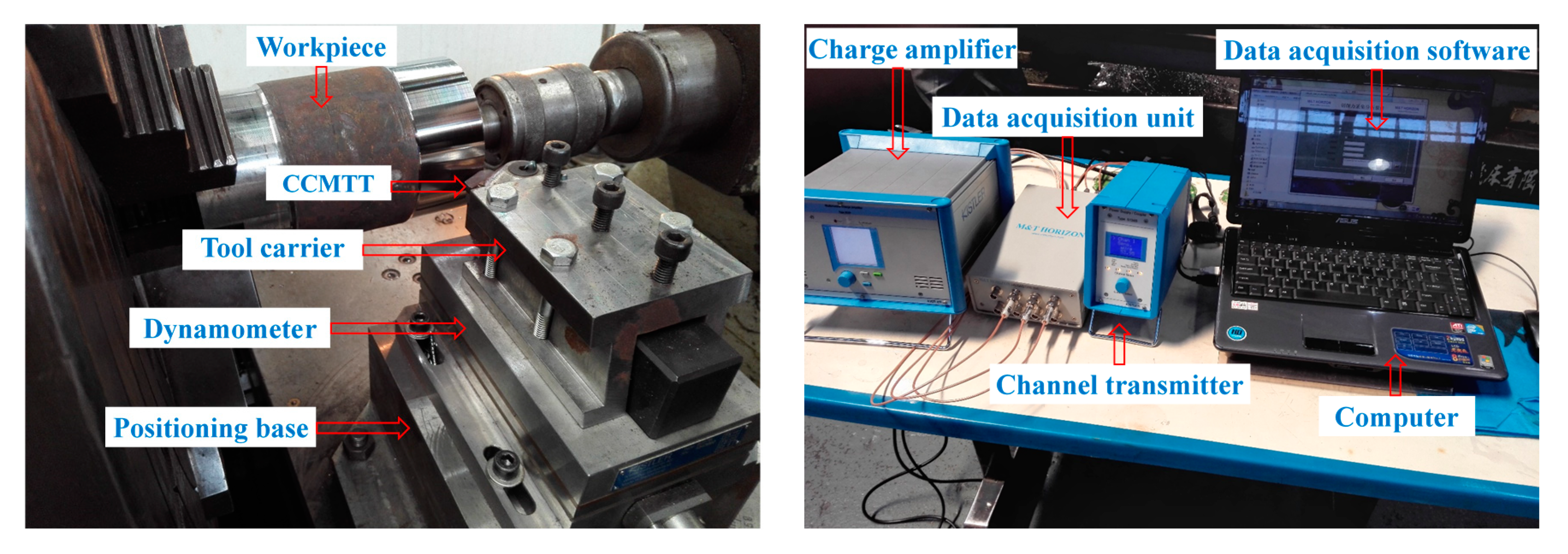
2.4. Experimental Conditions

The collection experiment on the impact load was carried out on a CW6163C lathe. By installing a Kistler three-dimensional dynamometer, the experimental platform was set up as shown in Figure 8. The cutting conditions were vc = 115 m/min, f = 0.42 mm/r and ap = 2 mm. The workpiece was oil country tubular goods (OCTG) 40CrMnMo, which is a high-strength alloy steel, as described above. The peak value of the cutting force of the CCMTT in three directions (the main cutting direction, the feed direction and the cutting depth direction) was measured and collected. The experiment was repeated five times, and the arithmetic mean value was taken as the effective data. The tool angles are shown in Table 1, and the mechanical properties of the tool and workpiece materials are shown in Table 2.
After collecting and processing the impact load in the cutting process, the test results were obtained, as shown in Table 3, which were used as the external input load of the PD numerical analysis of the CCMTT. The measurement uncertainties of cutting forces in three directions are all rather small, which illustrates that the test results are quite reliable.

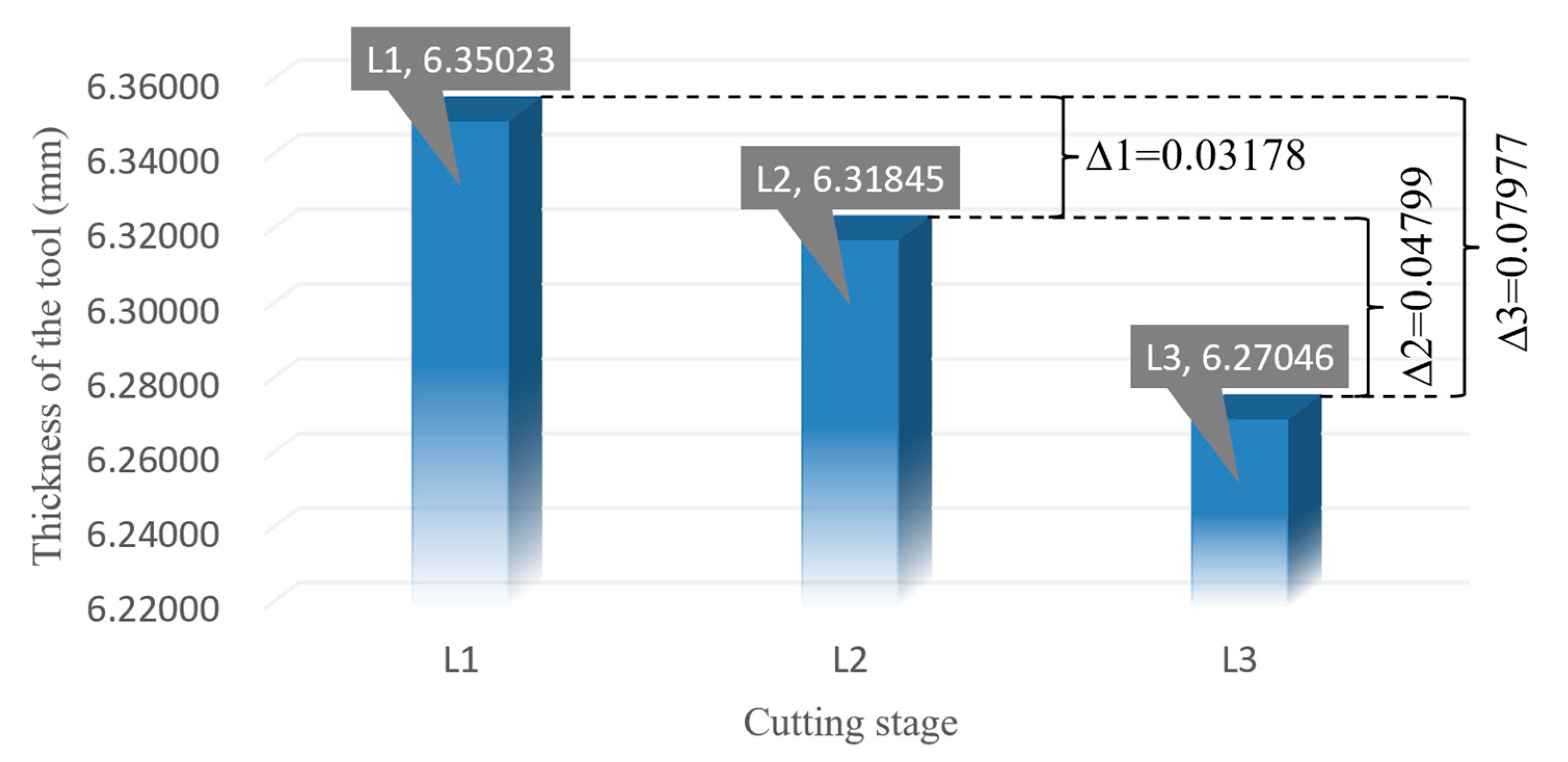
3. Analysis and Discussion

In the integrated environment of Microsoft Visual Studio 2015, using C++ programming language as the mathematical model expression medium, the PD theory was applied to analyze and predict the brittle damage of the CCMTT under an impact load in the cutting process.
On the premise of satisfying the stability of a numerical solution and combining it with the actual situation, the cycle index of the control program was controlled by defining the time step Δ t and the volume constant of the cubic lattice Δ x . According to the research needs, data were selectively exported. This paper focuses on the damage of the CCMTT, so the spatial positions (three-dimensional coordinates) of all discrete material points of the turning tool needed to be determined within certain calculation steps. The flow chart of the PD numerical analysis program of the CCMTT is shown in Figure 9.
When an object is in a relatively static state without an external effect, all of the material points inside it constitute an equilibrium system in a relatively static state. When the system is subjected to external action, the original equilibrium state is broken. Starting from the material point in the loaded area, there is obvious interaction among all material points in the system. Because the external action is only applied to the material points in a certain area of the system, the initial motion states of all material points in the system are different. When t = 0, the material point in the unloaded area is still in a relatively static state. The material points in the loaded area have acceleration, velocity and displacement, so the interactions between two different material points are different. Based on the PD model of the CCMTT, the time step of the numerical analysis was set to 3500. After the PD calculation, the spatial positions of discrete material points were output at the time steps 0, 1500, 2000, 2500, 3000 and 3500. The PD calculation was repeated three times, and the results were the same. By visualizing the PD analysis results of the CCMTT, the analysis results were obtained, as shown in Figure 10.
The process of crack generation and propagation is expressed by the displacement of material points in the near-field of the main cutting edge of the turning tool. Therefore, in the whole calculation process, three representative material points were selected from the external load area in the near-field of the cutting edge of the CCMTT to mark and track material point 1 on the main cutting edge, material point 2 on the flank face close to the main cutting edge and material point 3 on the neighboring layer downstream from the rake face adjacent to the main cutting edge. The displacements of three marker points above and near the cutting edge in the Y-direction (cutting depth direction), the Z-direction (main cutting direction) and the X-direction (feed direction) were studied. After data processing, the relationship curves between the displacements of three marked points in three directions and the calculation time steps were obtained after a 3500-time-step PD numerical solution for the CCMTT, as shown in Figure 11.
This paper focuses on the particle displacement caused by the damage to bonds between material points in the near-field of the cutting edge of the turning tool under the combined action of the main cutting force, axial thrust force and radial thrust force. It can be seen from Figure 11 that the displacements of the marked material points of the CCMTT in three directions do not just have a simple linear relationship with the calculation time, and there are fluctuations, especially in the direction of the feed and cutting depth, but the overall trend is that the displacement gradually increases with increasing calculation time, and the growth margin of material point displacement in the main cutting direction is the largest. The displacement of material points in the near-field of the cutting edge of the turning tool in the direction of the main cutting edge is the largest and most obvious, followed by the direction of the cutting depth, and the smallest in the direction of the feed. The displacement of material points is the result of the comprehensive influence of external loads and interaction forces between material points. From the phenomena above, it can be seen that the effect of external loads on the displacement of material points occupies the leading position. By analyzing the displacement of material points in three directions of the turning tool, it can be seen that the maximum displacements of the three marked material points of the CCMTT are 0.08431 mm, 0.007369 mm and 0.00444 mm, respectively, after 3500 steps of PD calculations. It can also be seen from Figure 11 that under the action of the external cutting loads generated under the given cutting conditions (vc = 115 m/min, f = 0.42 mm/r, ap = 2 mm), the material points in the near-field of the cutting edge of the CCMTT only have microdisplacements, which lead to microcracks, but the accumulation of microcracks at the material points has not reached the critical value of transformation. So, there are no macrocracks. However, it can be predicted that the corresponding microcracks will continuously accumulate according to the development speed of the microdisplacements. When the microcracks accumulate to a critical value of macro–micro transformation, macrocracks will be initiated, and the accumulation of macrocracks will lead to tool damage.
Material points move due to the action of external loads, and the “bonds” between material particles begin to deform, either compressing or stretching. When the elongation of the “bond” in the stretching state is greater than the ultimate elongation of the material s 0 , the “bond” will break, and the material particles at this point are more prone to relatively large displacements. In the whole calculation process, the maximum displacements in the Y-direction (direction of cutting depth), the Z-direction (main cutting direction) and the X-direction (feed direction) were analyzed. At the same time, in order to compare the displacements of material points in the near-field of the cutting edge in different directions, three groups of data were integrated and processed, and the displacement curves of the marked material point 1 in the X-, Y- and Z-directions were obtained, as shown in Figure 12.
From Figure 12, the same basic rule can be found: the maximum displacement occurs in the Z-direction, i.e., the main cutting direction, followed by the Y-direction, i.e., the direction of the cutting depth, and the minimum occurs in the X-direction, i.e., the feed direction. The margin increases with the increase in the load action time of the displacement of material points in the near-field of the cutting edge in the main cutting direction; i.e., the cutting time is significantly longer than those in the cutting depth and feed directions, and the main cutting direction with large incremental displacement is just the direction of the maximum load of the three-dimensional impact loads. The maximum displacement can reach 0.08232 mm. Based on the above analysis results, the damage in the main cutting direction of the CCMTT was further analyzed. Figure 13 shows the displacement of material points in the near-field of the cutting edge at different calculation time steps.
At the same time, a cutting experiment was carried out under the same cutting conditions, and the flank face of the CCMTT was observed and measured. The micromorphology of the flank face and the variation in the tool thickness in the near-field of the cutting edge in three stages are shown in Figure 14.
Figure 13 shows the position change in the main cutting direction of material points in the near-field of the cutting edge of the CCMTT at different stages of the whole PD numerical analysis process. The material points in the near-field of the cutting edge of the CCMTT have relatively obvious displacement in the main cutting direction under three-dimensional impact loads compared with the other two directions, but no obvious brittle cracks have occurred, which agrees well with the experimental results, as shown in Figure 14. Figure 14 shows that the change in the tool thickness in the near-field is still very small from the perspective of macrodeformation, that is, the displacement of the material points in the near-field of the cutting edge in the main cutting direction. The maximum displacement of material points in the main cutting direction in the cutting experiment reached 0.07977 mm, and it is not difficult to calculate a relative error of 3.2%. Meanwhile, from the total variation trend of the tool thickness shown in Figure 14, the experimental measurement results are basically consistent with the PD numerical analysis results. With the elapsing of the loading time, the number of integral “bonds” between material points gradually decreases, and the ratio φ ( x , t ) decreases accordingly. The damage extent of the material at particle x also deepens correspondingly, and microcracks continue to initiate, accumulate and propagate. When the proportion of integral “bonds” between material particles in the near-field of the cutting edge decreases to the breakage limit of the tool material, macroscopic breakage occurs.

4. Conclusions

The conclusions of this paper can be summarized as follows.
(1) The PD model of the CCMTT can be generated by establishing the boundary control mathematical model of the CCMTT, and the PD modeling accuracy of the whole CCMTT can be controlled within ± 3.4 % . The displacements of marked material points in three directions (the main cutting direction, the feed direction and the cutting depth direction) of the CCMTT do not have a linear relationship with the computation time, and there are fluctuations, especially in the directions of the feed and cutting depth. However, the overall trend is that the displacement gradually increases with the increase in the time of calculation, and the increment in the displacement of material points in the main cutting direction is the largest.
(2) The displacement of material points in the near-field of the cutting edge of the CCMTT is the largest and most obvious in the main cutting direction, followed by the direction of the cutting depth, and the smallest in the feed direction. The displacement of material points is the result of the comprehensive influence of the external load and the interaction force between material points. From the above phenomenon, it can be seen that the external load plays a dominant role in the displacement of material points.
(3) Under the given cutting conditions (vc = 115 m/min, f = 0.42 mm/r, ap = 2 mm), only microdisplacements of the material points in the near-field of the cutting edge of the CCMTT take place. The accumulation of microcracks resulting from the microdisplacement does not reach the critical point of transition, so a macrocrack is not formed. This agrees well with the experimental results, and the relative error can be controlled within 3.2%. It can be predicted that as the cutting process continues and the cutting load continues to be applied, the corresponding microcracks will continuously accumulate according to the development speed of the microdisplacement. When the microcracks accumulate to a certain critical value of macro–micro transformation, macrocracks will be initiated, and the continuous accumulation of macrocracks will lead to tool damage and failure.
(4) The simulation methodology is helpful to the numerical analysis and prediction of a tool’s brittle damage under an impact load in the cutting process of various materials. This research can provide a theoretical basis and reference for the selection and adjustment of cutting parameters in the material-cutting process. However, the methodology still has some limitations. It is insufficient for the universality of geometric modeling. At present, it is only applicable to objects with relatively simple geometric structures. It is difficult to model complex irregular surfaces. This is also the expected direction of the field of near-field dynamics in the future.

Author Contributions

Conceptualization, H.J. and Z.R.; methodology, H.J.; software, S.Y.; validation, Z.Z. and S.Y.; formal analysis, H.J.; investigation, Z.R.; resources, H.J.; data curation, Z.Z.; writing—original draft preparation, Z.Z.; writing—review and editing, Z.R. and H.J.; visualization, S.Y.; supervision, S.Y.; project administration, H.J. and Z.Z.; funding acquisition, H.J. All authors have read and agreed to the published version of the manuscript.

Funding

This work is financially supported by the National Natural Science Foundation of China (Grant No. 52005118, 52265055), the Science and Technology Plan Project of Guizhou Province (Grant No. QKHJC-ZK [2022]ZD026), the Science and Technology Plan Project of Guiyang City (ZKHT [2022]2-2) and the High-level Talents Research Initiation Fund of Guizhou Institute of Technology (Grant No. 2018073).

Data Availability Statement

Not applicable.

Conflicts of Interest

The authors declare no conflict of interest.

References

  1. Qian, F.; Ma, Y.L.; Wang, D.L.; Dong, H.M.; Gao, Y. Research and system development of tool breakage detection in production line. Univ. Politeh. Buchar. Sci. Bull. D Mech. Eng. 2017, 79, 217–234. [Google Scholar]
  2. Cho, H.S.; Han, J.-H.; Chi, S.-Y.; Yoo, K.-H. A tool breakage detection system using load signals of spindle motors in CNC machines. In Proceedings of the 2016 Eighth International Conference on Ubiquitous and Future Networks (ICUFN), Vienna, Austria, 5–8 July 2016; pp. 160–163. [Google Scholar] [CrossRef]
  3. Buchkremer, S.; Klocke, F.; Veselovac, D. 3D FEM simulation of chip breakage in metal cutting. Int. J. Adv. Manuf. Technol. 2015, 82, 645–661. [Google Scholar] [CrossRef]
  4. Lee, W.K.; Ratnam, M.M.; Ahmad, Z.A. Tool breakage detection from 2D workpiece profile using vision method. Mater. Sci. Eng. 2016, 114, 012132. [Google Scholar] [CrossRef]
  5. Mohamed, A.S.; Stephen, C.V. Effect of cutting speed on chipping and wear of the sialon ceramic tool in dry finish turning of the precipitation hardenable in 100 aerospace superalloy. J. Tribol. 2019, 141, 021604. [Google Scholar]
  6. Ma, C.; Wang, Z. Experimental and numerical investigation of the breakage of a cutting tool with ultrasonic vibration. Precis. Eng. 2018, 51, 393–402. [Google Scholar] [CrossRef]
  7. Chen, J.G.; Zheng, M.L.; Sun, Y.S.; Zhang, W.; Li, P.F. Research on the microscopic mechanism of the bond breakage of cemented carbide tools. J. Mech. Eng. 2018, 64, 726–742. [Google Scholar]
  8. Cheng, Y.-N.; Nie, W.-Y.; Guan, R.; Jia, W.-K.; Yan, F.-G. Study on damage behavior of carbide tool for milling difficult-to-machine material. Proc. Inst. Mech. Eng. Part C J. Mech. Eng. Sci. 2018, 233, 735–747. [Google Scholar] [CrossRef]
  9. Kresse, T.; Jürgens, W.; Meinhard, D.; Baumann, W.; Bernthaler, T.; Schneider, G. Wear and Damage Characterization of Coated Carbide Tools by means of FIB-SEM Microscopy. Pr. Met. 2018, 55, 704–715. [Google Scholar] [CrossRef]
  10. Cui, X.; Guo, J.; Zhao, J.; Yan, Y. Analysis of PCBN tool failure mechanisms in face milling of hardened steel using damage equivalent stress. Int. J. Adv. Manuf. Technol. 2015, 80, 1985–1994. [Google Scholar] [CrossRef]
  11. Jiang, H.W.; He, L.; Fan, L.; Zhao, X.F.; Zhan, G. Peridynamic theory-based prediction of micro breakage of cemented carbide tool. J. South China Univ. Technol. (Nat. Sci. Ed.) 2016, 44, 8–15. [Google Scholar]
  12. Jiang, H.; He, L.; Fan, L.; Zhan, G. Numerical analysis method of cemented carbide turning tool’s micro breakage based on peridynamic theory. Int. J. Adv. Manuf. Technol. 2016, 88, 1619–1628. [Google Scholar] [CrossRef]
  13. Silling, S.A.; Weckner, O.; Askari, E.; Bobaru, F. Crack nucleation in a peridynamic solid. Int. J. Fract. 2010, 162, 219–227. [Google Scholar] [CrossRef]
  14. Le, Q.V.; Bobaru, F. Surface corrections for peridynamic models in elasticity and fracture. Comput. Mech. 2017, 61, 499–518. [Google Scholar] [CrossRef]
  15. Liu, W.; Yang, G.; Cai, Y. Modeling of failure mode switching and shear band propagation using the correspondence framework of peridynamics. Comput. Struct. 2018, 209, 150–162. [Google Scholar] [CrossRef]
  16. Pashazad, H.; Kharazi, M. A peridynamic plastic model based on von Mises criteria with isotropic, kinematic and mixed hardenings under cyclic loading. Int. J. Mech. Sci. 2019, 156, 182–204. [Google Scholar] [CrossRef]
  17. Zaccariotto, M.; Mudric, T.; Tomasi, D.; Shojaei, A.; Galvanetto, U. Coupling of FEM meshes with Peridynamic grids. Comput. Methods Appl. Mech. Eng. 2018, 330, 471–497. [Google Scholar] [CrossRef]
  18. Jafari, A.; Ezzati, M.; Atai, A.A. Static and free vibration analysis of Timoshenko beam based on combined peridynamic-classical theory besides FEM formulation. Comput. Struct. 2019, 213, 72–81. [Google Scholar] [CrossRef]
  19. Wang, Y.; Zhou, X.; Wang, Y.; Shou, Y. A 3-D conjugated bond-pair-based peridynamic formulation for initiation and propagation of cracks in brittle solids. Int. J. Solids Struct. 2018, 134, 89–115. [Google Scholar] [CrossRef]
  20. Zhang, G.; Gazonas, G.A.; Bobaru, F. Supershear damage propagation and sub-Rayleigh crack growth from edge-on impact: A peridynamic analysis. Int. J. Impact Eng. 2018, 113, 73–87. [Google Scholar] [CrossRef]
  21. Alali, B.; Gunzburger, M. Peridynamics and Material Interfaces. J. Elast. 2015, 120, 225–248. [Google Scholar] [CrossRef]
  22. Diana, V.; Casolo, S. A full orthotropic micropolar peridynamic formulation for linearly elastic solids. Int. J. Mech. Sci. 2019, 160, 140–155. [Google Scholar] [CrossRef]
  23. Shojaei, A.; Mossaiby, F.; Zaccariotto, M.; Galvanetto, U. An adaptive multi-grid peridynamic method for dynamic fracture analysis. Int. J. Mech. Sci. 2018, 144, 600–617. [Google Scholar] [CrossRef]
  24. Silling, S. Stability of peridynamic correspondence material models and their particle discretizations. Comput. Methods Appl. Mech. Eng. 2017, 322, 42–57. [Google Scholar] [CrossRef]
  25. Kovalchenko, A.M.; Goel, S.; Zakiev, I.M.; Pashchenko, E.A.; Al-Sayegh, R. Suppressing scratch-induced brittle fracture in silicon by geometric design modification of the abrasive grits. J. Mater. Res. Technol. 2018, 8, 703–712. [Google Scholar] [CrossRef]
  26. Garcia, J.M.; Brandao, L.P.; Costa, U.O.; Salgado, J.V.; Nunes, L.F.; Paula, A.D.S.; Monteiro, S.N. Experimental creep behavior and life prediction through observation and numerical analysis for AISI 310. J. Mater. Res. Technol. 2019, 9, 222–229. [Google Scholar] [CrossRef]
  27. Dabees, S.; Tirth, V.; Mohamed, A.; Kamel, B.M. Wear performance and mechanical properties of mwcnt/hdpe nanocomposites for gearing applications. J. Mater. Res. Technol. 2020, 12, 2476–2488. [Google Scholar]
  28. Zhang, H.; Li, H.; Ye, H.; Zheng, Y. A coupling peridynamic approach for the consolidation and dynamic analysis of saturated porous media. Comput. Mech. 2019, 64, 1097–1113. [Google Scholar] [CrossRef]
  29. Anbarlooie, B.; Hosseini-Toudeshky, H. Peridynamic micromechanical prediction of nonlocal damage initiation and propagation in DP steels based on real microstructure. Int. J. Mech. Sci. 2019, 153–154, 64–74. [Google Scholar] [CrossRef]
  30. Madenci, E.; Barut, A. Futch M Peridynamic differential operator and its applications. Comput. Methods Appl. Mech. Eng. 2016, 304, 408–451. [Google Scholar]
  31. Silling, S.; Littlewood, D.; Seleson, P. Variable horizon in a peridynamic medium. J. Mech. Mater. Struct. 2015, 10, 591–612. [Google Scholar] [CrossRef]
  32. Shojaei, A.; Mudric, T.; Zaccariotto, M.; Galvanetto, U. A coupled meshless finite point/Peridynamic method for 2D dynamic fracture analysis. Int. J. Mech. Sci. 2016, 119, 419–431. [Google Scholar] [CrossRef]
  33. Silling, S. Solitary waves in a peridynamic elastic solid. J. Mech. Phys. Solids 2016, 96, 121–132. [Google Scholar] [CrossRef]
  34. Oterkus, S.; Madenci, E. Peridynamic modeling of fuel pellet cracking. Eng. Fract. Mech. 2017, 176, 23–37. [Google Scholar] [CrossRef]
  35. Hu, Y.; Madenci, E. Bond-based peridynamic modeling of composite laminates with arbitrary fiber orientation and stacking sequence. Compos. Struct. 2016, 153, 139–175. [Google Scholar] [CrossRef]
  36. Yaghoobi, A.; Chorzepa, M.G. Fracture analysis of fiber reinforced concrete structures in the micropolar peridynamic analysis framework. Eng. Fract. Mech. 2017, 169, 238–250. [Google Scholar] [CrossRef]
  37. Du, Q.; Tao, Y.; Tian, X. A Peridynamic Model of Fracture Mechanics with Bond-Breaking. J. Elast. 2017, 132, 197–218. [Google Scholar] [CrossRef]
  38. John, T.; Xu, X. A generalized, ordinary, finite deformation constitutive correspondence model for peridynamics. Int. J. Solids Struct. 2018, 141, 245–253. [Google Scholar]
  39. Madenci, E.; Diyaroglu, C.; Anicode, V.; Silling, S. Peridynamic Modeling of Drilling Process in Polymer Matrix Composites. In Proceedings of the AIAA SciTech 2019 Forum, San Diego, CA, USA, 7–11 January 2019. [Google Scholar] [CrossRef]
Figure 1. Interaction and motion state between material points: (a) reference domain and reference subdomain, (b) motion vector relation of material point and (c) interaction between material points in near-field.
Processes 11 00520 g001aProcesses 11 00520 g001b
Figure 2. PD computational domain: (a) ideal region and (b) actual PD region.
Processes 11 00520 g002
Figure 3. Geometric model of the CCMTT: (a) 3D model of the CCMTT and (b) geometric shape and key parameters of the CCMTT.
Processes 11 00520 g003
Figure 4. Analysis of calculation accuracy and efficiency: (a) relationship between calculation area and cubic lattice and (b) relationship between iteration times and cubic lattice.
Processes 11 00520 g004
Figure 5. Calculation model of the CCMTT: (a) i-j coordinate system and (b) i-k coordinate system.
Processes 11 00520 g005
Figure 6. PD model of the CCMTT: (a) region 1 and (b) region 2.
Processes 11 00520 g006
Figure 7. Loaded area of CCMTT in cutting simulation.
Processes 11 00520 g007
Figure 8. Test platform of cutting force collection.
Processes 11 00520 g008
Figure 9. Flow chart of PD numerical analysis program of brittle damage of a turning tool.
Processes 11 00520 g009
Figure 10. PD analysis results after 3500 iterations of the CCMTT.
Processes 11 00520 g010
Figure 11. Displacement changing with the time of material points marked in the near-field of the cutting edge: (a) feed direction, (b) cutting depth direction and (c) main cutting direction.
Processes 11 00520 g011
Figure 12. Contrast curve of maximum displacement of material points in three directions.
Processes 11 00520 g012
Figure 13. Position evolution in the main cutting direction of material points of the CCMTT: (a) the first step of PD analysis of the CCMTT (initial state), (b) the 2000th step of PD analysis of the CCMTT (microdisplacement), (c) the 3500th step of PD analysis of the CCMTT (further microdisplacement).
Processes 11 00520 g013
Figure 14. Variation in tool thickness in the near-field of the CCMTT in different stages.
Processes 11 00520 g014
Table 1. Geometric angles of the tool.
Geometric Angle Tool   Tip   Angle   ε r Clearance   Angle   α 0 Main   Cutting - Edge   Angle   k r End   Cutting - Edge   Angle   k r Inclination   Angle   λ s Approach   Angle   ψ r
Value (°)150727.52.5062.5
Table 2. Property parameters of tool and workpiece materials.
Material Density   ( g / c m 3 ) Tensile Strength (MPa)Bending Strength (MPa)HardnessPoisson’s RatioElastic Modulus (GPa)
Tool13.8784.5 118091.8HRA0.23540–600
Workpiece7.871080\30HRC0.28212
Table 3. Impact force collected from cutting experiments.
Cutting ForceMain Cutting Force
Fc (N)
Axial Thrust Force
Ff (N)
Radial Thrust Force
Fp (N)
Test Number
12104.58953.211103.56
22235.12980.431086.31
32085.75897.651018.15
42116.23958.321132.46
52201.87962.541107.29
Average value2148.71950.431089.55
Uncertainty−9.0949E-144.55E-141.13687E-13
Disclaimer/Publisher’s Note: The statements, opinions and data contained in all publications are solely those of the individual author(s) and contributor(s) and not of MDPI and/or the editor(s). MDPI and/or the editor(s) disclaim responsibility for any injury to people or property resulting from any ideas, methods, instructions or products referred to in the content.

