Abstract
Many multi-objective optimization problems in the real world have conflicting objectives, and these objectives change over time, known as dynamic multi-objective optimization problems (DMOPs). In recent years, transfer learning has attracted growing attention to solve DMOPs, since it is capable of leveraging historical information to guide the evolutionary search. However, there is still much room for improvement in the transfer effect and the computational efficiency. In this paper, we propose a cluster-based regression transfer learning-based dynamic multi-objective evolutionary algorithm named CRTL-DMOEA. It consists of two components, which are the cluster-based selection and cluster-based regression transfer. In particular, once a change occurs, we employ a cluster-based selection mechanism to partition the previous Pareto optimal solutions and find the clustering centroids, which are then fed into autoregression prediction model. Afterwards, to improve the prediction accuracy, we build a strong regression transfer model based on TrAdaboost.R2 by taking advantage of the clustering centroids. Finally, a high-quality initial population for the new environment is predicted with the regression transfer model. Through a comparison with some chosen state-of-the-art algorithms, the experimental results demonstrate that the proposed CRTL-DMOEA is capable of improving the performance of dynamic optimization on different test problems.
1. Introduction
In the real world, many multi-objective optimization problems [1] have multiple conflicting objectives that may change over time. Such problems are called dynamic multi-objective optimization problems (DMOPs) [2]. In recent years, the research on solving DMOPs has attracted more and more researchers and there have been lots of optimization methods developed [3,4,5]. Multi-objective evolutionary algorithms (MOEAs) have been widely applied to solve DMOPs in various areas, such as wireless sensor networks [6], financial optimization problems [7], path planning [8] and so on. When applied to solve DMOPs, traditional MOEAs [9,10,11,12] should be improved to adapt to the dynamisms, which are capable of tracking the changing Pareto optimal fronts (POFs) and providing a diverse set of Pareto optimal solutions (POSs) over time.
To solve DMOPs, there are various kinds of dynamic MOEAs (DMOEAs) in the literature, which can be categorized as follows: diversity approaches [13,14,15], memory mechanisms [16,17,18], and prediction-based methods [19,20,21]. Generally, the diversity approaches include increasing diversity [22], maintaining diversity [15], and multi-population strategy [23]. More specifically, the environmental adaption of population diversity can be addressed with increasing diversity by adding variety to the population after the detection of a change, maintaining diversity by avoiding population convergence to track the time-varying POS throughout the run, or dividing the population into some different subpopulations. Additionally, a variety of memory mechanisms are designed to store historical information in the past environment and reuse these information so as to save computational costs or guide the future search direction.
Among various DMOEAs, the prediction-based methods take advantage of the previous search information to predict future POSs and have drawn lots of attention recently. [24] proposed a feed-forward prediction strategy to estimate the new POS, aiming at improving the convergence speed to the new POF. However, this strategy ignores the distribution characteristics of POF and affects the prediction efficiency. Zhou et al. [25] put forward a novel prediction-based population re-initialization method to predict the new locations of optimal solutions when a change occurs.
In recent years, transfer learning [26,27] has been considered to be capable of effectively improving the prediction performance. For DMOPs, the dynamic nature at two adjacent time steps may share certain common features, and thereby the solutions obtained from the previous environment can provide useful knowledge for the new individuals during the optimization process. Jiang et al. [28] proposed a DMOEA based on transfer learning, named Tr-DMOEA, to predict an initial population by learning from the previous evolutionary process. In their work, transfer component analysis (TCA) [29] is applied to find a latent space where the objective values of solutions in the target domain are close to that of solutions in the source domain. Besides, to improve the computational efficiency, several transfer learning-based DMOEAs have been presented in [30,31,32], where the promising solutions in the new environment are predicted with the historical information of past environments using individual-based methods [32], manifold transfer learning [31], knee point-based imbalanced transfer learning [30], etc.
Even though remarkable progress has been made in transfer learning-based DMOEAs, there is still much room for improvement in the transfer performance. First, as mentioned in [32], transferring a large number of common solutions consumes a large amount of computational resources, and the negative transfer can easily occur due to solution aggregation. Second, most of the existing algorithms transfer knowledge through a latent space that requires more parameters and takes excessive computing time.
In view of the above shortcomings, we propose a cluster-based regression transfer learning method-based DMOEA, called CRTL-DMOEA, which consists of two stages, i.e., cluster-based selection and cluster-based regression transfer. Specifically, once a change occurs, the cluster-based selection mechanism is first employed to find the centroids of approximate POSs by clustering the previous POSs with localPCA [33], which are then fed into autoregression (AR) [34] model. Afterwards, to improve the prediction accuracy, we build an regression transfer model based on TrAdaboost.R2 [35] by taking advantage of the knowledge from the clustering centroids. Finally, a high-quality initial population is predicted with the assistance of the regression transfer model for the new environment.
The main contributions of this paper are given as follows:
- In this paper, we present a cluster-based selection mechanism by clustering the previous POSs with localPCA, and predicting the centroids in each cluster with AR model. Selecting the representative individuals to transfer can save a lot of computational time and the effect of transfer.
- This paper proposes a cluster-based regression transfer method based on the TrAdaboost.R2 to leverage the information from clustered centroids in historical environment. The method constructs a regression transfer model, which does not need setting more hyperparameters and improve the computational complexity.
- The proposed algorithm has been shown to be effective by comparing with other state-of-the-art methods on different types of benchmark problems.
Section 2 introduces the background and related work. Section 3 elaborates on CRTL-DMOEA in detail. Section 4 presents the experimental design and results. Section 5 concludes and discusses future research.
2. Background and Related Work
2.1. Dynamic Multi-Objective Optimization
Without the loss of generality, we consider the minimization problem and the DMOP is mathematically defined as follows:
where is the n-dimension decision variable bounded in the decision space . t represents the environment variable. denotes the M-dimensional objective vector.
Definition 1.
(Dynamic Pareto Dominance): At time t, is said to Pareto dominate , denoted by , if and only if
Definition 2.
(Dynamic Pareto Optimal Set (DPOS)): If a solution is not dominated by any other solution, is called a Pareto optimal solution. All at time t form the DPOS, denoted by
Definition 3.
(Dynamic Pareto Optimal Front (DPOF)): is the objective function with respect to time t. DPOF is defined as follows:
2.2. Related Work
At present, the key components of DMOEAs are environmental change detection, change response strategy and static multi-objective EA (MOEA). The environmental change detection is mainly used to detect whether change occurs in the environment. The state-of-the-art research mainly focuses on three aspects, including re-evaluation [3,22,34,36], distribution estimation of objective value [37], and steady-state detection [38]. In general, the most common detection mechanism is performed to re-evaluate the best solution, or some other solutions as detectors. If the objective values are different in adjacent times, we judge that the change has been detected. Jiang et al. [38] proposed a steady-state change detection method based on re-evaluation. Instead of selecting a proportion of population members as sentinels, they check the whole population in random order one by one. Afterwards, a change is assumed to be detected if a discrepancy is found in one member and there is no need to do further evaluation.
In the literature, various change response strategies have been proposed to track the POS of the new environment quickly by initializing the population and respond to the changed environment in time, which are the core component of DMOEAs. Generally, they can be mainly classified as follows: diversity approaches [13,14,15], memory mechanisms [16,17,18], and prediction-based methods [19,20,21].
The diversity approaches handle DMOPs by increasing diversity [22] and maintaining diversity [15], as well as through multi-population strategies [23]. The increasing diversity methods generally take some explicit actions such as reinitialization or hypermutation when a change occurs. Jiang et al. [38] proposed a change respond mechanism to maintain a balanced level of population diversity and convergence. The increasing diversity methods blindly respond to the changing environment, probably resulting in misleading the optimization process. Most of the maintaining diversity methods tend to keep a certain level of diversity and thereby adapt more easily to changes and explore the new search space. Grefenstette [13] proposed a random immigrant generic algorithm to replace some individuals by randomly generated ones in every generation. Multi-population approach is to maintain multiple sub-populations at the same time and do the exploration or exploitation tasks separately. This kind of approaches is known to be effective for solving multiple peaks or the competing peaks problems. Wang et al. [39] proposed that multiple sub-populations can be generated adaptively based on a set of single-objective sub-problems decomposed from a MOP.
As for the memory mechanisms, Yang [40] proposed an associative memory scheme for genetic algorithms, in which both the optimal individuals and the environmental information are stored in the memory and leveraged to generate a new population when a change has been recognized. Goh and Tan [3] proposed a competitive–cooperative co-evolutionary algorithm for DMOPs, in which a temporary memory method is used to store the previous solutions in the archive.
Significantly, the prediction-based methods have shown to be effective to reuse the historical information to predict the future individuals in handling DMOPs. Koo et al. [41] proposed a gradient strategy for DMOPs which predicts the direction and magnitude of the next change based on the historical solutions. However, such methods assume that the training and test data should have the same distribution, which may not become true in many real-world DMOPs. Integrating transfer learning into DMOEAs [42,43] is effective to address this issue, which could improve the learning performance by avoiding much expensive efforts in data labeling. However, to further improve the computationally intensive property and overcome the negative transfer remain great challenges when dealing with DMOPs.
3. Proposed Methods
In this section, we propose a cluster-based regression transfer learning method-based DMOEA, called CRTL-DMOEA, to handle DMOPs. Two main components, i.e., cluster-based selection and cluster-based regression transfer, as shown in Figure 1, are unified into one framework to generate an excellent initial population to help the MOEA find the changing POS efficiently and effectively.
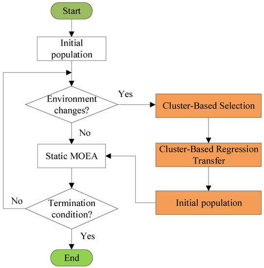
Figure 1.
The diagram of the proposed CRTL-DMOEA.
The schematic of the proposed CRTL-DMOEA is provided in Figure 2. Briefly, CRTL-DMOEA randomly initializes the population. If an environmental change is detected, the cluster-based selection mechanism is first employed to find the centroids of approximate POSs and estimate the centroids under new environment with AR model. Subsequently, an regression transfer model based on TrAdaboost.R2 [35] is constructed to transfer the knowledge from the estimated centroids and obtain a high-quality initial population for the new environment. Finally, the new generated initial population are optimized by static MOEAs to converge towards POSs at different environments.
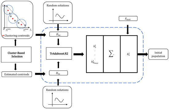
Figure 2.
The schematic of the proposed CRTL-DMOEA.
3.1. The Overall Framework
The pseudo-code of CRTL-DMOEA is given in Algorithm 1. In the following, we will describe the overall framework in detail.
- Line 1-2: The initial population is randomly generated in the decision space and optimized by MOEA.
- Line 3: Check for environmental changes.
- Line 4: The time t is increased by 1, if the environment changes.
- Line 5: The clustering centroids C and corresponding estimated centroids are found by Cluster-Based Selection, which will be described in Section 3.2.
- Line 6: Two sets of population and are randomly generated.
- Line 7-8: The clustering centroids and , together with their objective values at time are regarded as the source domain .
- Line 9-10: The estimated centroids and are merged with their current objective values to serve as the target domain .
- Line 11: Cluster-Based Regression Transfer utilizes and to generate the initial population , which will be described in Section 3.3.
- Line 12: will be further optimized by MOEA.
| Algorithm 1 The framework of CRTL-DMOEA. |
| Input:: the dynamic optimization problem; MOEA: a static MOEA; : the number of clusters. |
| Output: The POS of in different environments. |
| 1: Randomly initialize N individuals ; |
| 2: = MOEA; |
| 3: while change detected do |
| 4: ; |
| 5: = Cluster-Based Selection; |
| 6: Generate randomly two sets of solutions and ; |
| 7: ; |
| 8: ; |
| 9: ; |
| 10: ; |
| 11: = Cluster-Based Regression Transfer; |
| 12: = MOEA; |
| 13: end while |
3.2. Cluster-Based Selection
The goal of cluster-based selection is to generate the estimated centroids, which are used to construct the transfer model in the next step. We use localPCA [33] to cluster the previous POS and find the centroids with excellent convergence and diversity, which are then predicted by AR [34] model to obtain the estimated centroids.
To depict the procedure of cluster-based selection, the pseudo-code is given in Algorithm 2. Firstly, we set the clustering centroids and estimated centroids as empty set in line 1. Then, localPCA was applied to partition the previous approximate into subpopulation in line 2. Specifically, we partitioned the individuals in into disjoint clusters according to the distances from the individual to the principal subspace of the points in each cluster. Afterwards, in line 4, the centroid of cluster can be obtained by
where stands for the kth individual in cluster and means the cardinality. All the in each cluster form the set of clustering centroids C in line 5. Subsequently, the AR model was constructed for prediction in line 6, with more details introduced in [34]. Finally, we obtained the estimated centroids in line 7, which were subsequently used to train the regression transfer model for the new environment.
| Algorithm 2 Cluster-Based Selection. |
| Input:: the dynamic optimization problem; : the POS at time ; : the number of clusters. |
| Output: The set of clustering centroids and estimated centriods C and . |
| 1: Set and ; |
| 2: Clustering into , , by localPCA; |
| 3: for do |
| 4: Calculate the centroid of each cluster by Equation (5); |
| 5: ; |
| 6: Predict the clustering centroids by AR model and obtain estimated centroid ; |
| 7: ; |
| 8: end for |
| 9: return; |
3.3. Cluster-Based Regression Transfer Method
In this section, we propose a cluster-based regression transfer method based on TrAdaboost.R2. Our motivation is to save the computational cost while improving the transfer effect. This method constructs a strong regression model at time t, which can be used to filter out a high-quality initial population for the next time moment.
In the following, we will describe the details of this method as shown in Algorithm 3. The source domain consists of the clustering centroids, , and their objective values at time . The target domain includes the estimated centroids , and their objective values at time t.
- Line 1: The initial population is an empty set.
- Line 2: and are merged into one set D.
- Line 3-4: Initialize the weight for all individuals and set the number of iterations .
- Line 5-10: weak regression models are trained with TrAdaboost.R2.
- Line 11: The strong regression model is constructed by combining the final weak models.
- Line 12-13: We randomly sample a large number of test samples , which are predicted by the regression model to get the predicted objective values .
- Line 14: are ranked by non-dominated sorting based on the estimated objective values, and the non-dominated solutions are stored as .
- Line 15-20: If the size of exceeds N, we randomly select some solutions to truncate; otherwise, some Gaussian noises will be added.
- Line 21: serves as the initial population for the static MOEA to be optimized in the new environment.
More specifically, when constructing the weak regression models with TrAdaboost.R2, the weight is firstly initialized as for each individual. Then, to train each weak regression models , we call a base learner Support Vector Regression (SVR) [44] with D and . The error between the true objective value and the weak regression model are mapped into an adjusted error , which is expressed as:
where
After that, we calculate the adjusted error for by
Then, the weight for each individual is updated based on the adjusted error and . We treat the training data in D differently, which means that, if an individual have a large adjusting error , we increase its weight if it belongs to and decrease its weight if it is from . The update of weights can be calculated as
where
Following this, the individuals with large weights are adapted to the target domain, which is helpful for the base learner to train subsequent regression models.
| Algorithm 3 Cluster-Based Regression Transfer. |
| Input:: the source data set; : the target data set; : the number of clusters; N: the population size. |
| Output: The initial population . |
| 1: Set ; |
| 2: ; |
| 3: Initialize the weight for all individuals; |
| 4: Set the number of iterations ; |
| 5: for to do |
| 6: Use SVR to train a weak regression model with D and ; |
| 7: Compute the adjusted error by Equation (6) for each individual; |
| 8: Compute the adjusted error of by Equation (8); |
| 9: Update the weight by Equation (9); |
| 10: end for |
| 11: Obtain the strong regression model by combining the final weak models; |
| 12: Randomly generate a large number of test solutions ; |
| 13: Apply to predict the objective value ; |
| 14: Find non-dominated solutions in ; |
| 15: while do |
| 16: Delete individual in ; |
| 17: end while |
| 18: while do |
| 19: Add Gaussian noises to ; |
| 20: end while |
| 21: return ; |
3.4. Computational Complexity
In CRTL-DMOEA, the computational costs are mainly spent on the process of clustering, non-dominated sorting, and regression transfer method. Clustering by localPCA consumes , where d is the dimension of decision variables. The complexity of the non-dominated sorting is , where M is the number of objectives. In the regression transfer method, the computational complexity of obtaining the strong classifier is .
4. Experimental Studies
4.1. Test Problems
In the experiment, we use the widely used FDA [45], dMOP [3], and F test suite [34] to evaluate all compared algorithms. The FDA test suit consists of five DMOPs, i.e., FDA1-FDA5, which are linearly related between decision variables. The dMOP test suite is proposed by extending the FDA test suite. Moreover, F5-F10 problems in F test suit have more complex dynamic geometries than others over time.
According to the different dynamical changes of DPOS and DPOF, DMOPs can be classified into four types:
- TYPE I: The POS changes over time, but the POF is fixed.
- TYPE II: Both the POS and POF change over time.
- TYPE III: The POS is fixed while the POF changes.
- TYPE IV: Both the POS and POF are fixed, but the problem changes.
Based on the classification mentioned above, FDA1, FDA4, and dMOP3 belong to Type I problem. FDA3, FDA5, dMOP2 and F5-F10 belong to Type II problem. FDA2 and dMOP1 belong to Type III problem. In these DMOPs, the time variable t is defined as:
where and refer to the severity and frequency of changes. is the generation counter.
4.2. Compared Algorithms and Parameter Settings
The proposed CRTL-DMOEA is compared with four other popular algorithms, including MOEA/D-KF [46], PPS [34] Tr-MOEA/D [28] and KT-MOEA/D [30]. MOEA/D-KF and PPS are prediction-based DMOEAs, while Tr-MOEA/D and KT-MOEA/D are based on transfer learning. The algorithms are implemented in MATLAB R2020a on an Intel Core i7 with 2.70 GHz CPU on Windows 10. For a fair comparison, most parameters follow the original references. Other common parameters are summarized below:
- In the experiments, the population size N is set to 100 for biobjective optimization problems and 150 for triobjective problems. The number of decision variables n is set as 10.
- There are three pairs of dynamic configurations, which are (), (), and (). The total number of generations is set to .
- In CRTL-DMOEA, the cluster number is 10, and MOEA/D [47] is used as the static optimizer.
- Each algorithm is run 20 times independently on each test problem.
4.3. Performance Metrics
4.3.1. Modified Inverted Generational Distance (MIGD)
The inverted generational distance (IGD) [33] is a commonly used metric to assess the performance of MOEAs in terms of convergence and diversity of the obtained solutions. A smaller IGD value indicates better convergence and higher diversity. Mathematically, the IGD is computed as:
where is uniformly distributed points along the true POF. POF denotes the approximated POF obtained by a MOEA. Additionally, is the Euclidean distance between the point and p.
The MIGD metric is defined as the average of IGD values over all time steps over a run, i.e.,
where T is a set of discrete time steps in a run.
4.3.2. Modified Hypervolume (MHV)
The hypervolume (HV) [25] is a metric that takes into account convergence and distribution of solutions simultaneously in order to evaluate the comprehensive quality of the obtained POF. A larger HV value indicates the better convergence and distribution. Like MIGD modified from IGD, MHV is defined as the average of the HV values in all time steps over a run.
4.4. Comparison with Other DMOEAs
In this section, we conduct the performance comparisons of all algorithms in solving different types of DMOPs, including FDA, dMOP and F problems described in Section 4.1. The statistical results on MIGD values obtained by compared algorithms are presented in Table 1. In this table, the symbols and denote that the proposed CRTL-MOEA/D performs significantly better and worse than compared algorithm, respectively, while the symbol means there is no significant difference by utilizing the Wilcoxon rank sum test [48] at a significance level of 0.05.

Table 1.
MIGD values obtained by five algorithms on different test problems.
As can be seen from Table 1, CRTL-MOEA/D achieves 32 out of 42 best results on FDA, dMOP and F test problems in terms of MIGD metric. CRTL-MOEA/D shows slightly worse than KT-MOEA/D on F5, F7 and F8. However, CRTL-MOEA/D performs significantly worse on FDA5 and F10 problems, which is possibly due to the complex characteristics of these problems. In FDA5, both the geometric shapes of POF and POS are not fixed in dynamic environment. In F10, the POS occasionally jumps from one area to another one and two adjacent POFs are different. The complications make it difficult to acquire valid historical knowledge for building a regression transfer model to generate a high-quality initial population when the change occurs.
To visually show the comprehensive performance of all algorithms at different environments, we plot the average logarithmic IGD in the first 20 changes with in Figure 3. It is clear to see that, compared with other algorithms, CRTL-MOEA/D achieves better IGD results and stability with time.
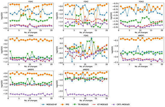
Figure 3.
Average log(IGD) obtained by five algorithms on FDA and dMOP problems.
Besides, to qualify the significant differences, Figure 4 gives the average performance rankings with Friedman test [49] with regard to MIGD. A lower average performance score indicates a better overall performance. As observed from Figure 4, CRTL-MOEA/D has the best score 1.40, indicating the better performance than MOEA/D-KF (3.35), PPS (4.71), Tr-MOEA/D (3.29), and KT-MOEA/D (2.25). Moreover, we take another post-hoc Nemenyi test [49] to plot the critical difference (CD) in Figure 5, which shows the significance of paired differences among all algorithms. It shows that CRTL-MOEA/D is only comparable to KT-MOEA/D while significantly different from others. Besides, MHV results are provided in Table 2. From all the experimental results, we can conclude that CRTL-DMOEA is more effective than other algorithms to track the time-varying POS in terms of convergence and diversity on most test cases.
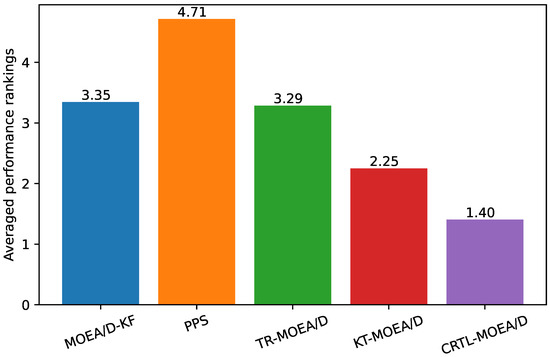
Figure 4.
The Friedman ranks of five compared algorithms on the MIGD values.
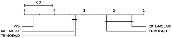
Figure 5.
CD plot of five compared algorithms.
Table 2.
MHV values obtained by five algorithms on different test problems.
4.5. Ablation Study
The proposed CRTL-MOEA/D has two key components: cluster-based selection and cluster-based regression transfer. To validate the effectiveness of these two mechanisms, an ablation experiment is carried out by comparing CRTL-MOEA/D with two variants (CRTL-MOEA/D and CRTL-MOEA/D) on different problems with and . CRTL-MOEA/D utilizes the estimated clustering centroids and random solutions to form the initial population without regression transfer learning. In CRTL-MOEA/D, the centriod selection is removed. The previous POSs and their objective values are treated as the source domain for regression transfer. The random solutions generated in the new environment and objective values are used as the target domain.
The statistical results on MIGD valus are provided in Table 3. From Table 3, it is clear to see that CRTL-MOEA/D shows superior performance over CRTL-MOEA/D on most cases, indicating that the cluster-based regression transfer contributes to exploit informative historical knowledge to generate a high-quality initial population for the new environment. In addition, CRTL-MOEA/D surpasses CRTL-MOEA/D on most problems. Thus, we can conclude that it is more effective to transfer clustering centroids than all the non-dominated solutions. In addition, CRTL-MOEA/D obtains the best results in 6 out of 8 cases, which also shows the effectiveness of combining these two components.
Table 3.
MIGD values obtained by CRTL-MOEA/D, CRTL-MOEA/D and CRTL-MOEA/D.
4.6. Running Time
In this section, we compare the running time of different algorithms and provide the results in Table 4. As observed in the table, CRTL-DMOEA has smaller running time than other algorithms on most of test instances. This shows that the proposed cluster-based selection and regression transfer method are very efficient. Tr-MOEA/D needs more running time than CRTL-DMOEA. The main reason behind this is that CRTL-DMOEA selects the representative individuals to transfer, rather than all optimal solutions used in Tr-MOEA/D, which can save a lot of running time. Besides, Tr-MOEA/D needs more parameters to build the latent space, which takes , where L is the total number of bits of the input. However, CRTL-DMOEA constructs an essentially sample-based regression model, which can avoid the need for more parameter settings and improve the computational complexity. To summarize, CRTL-DMOEA seems competitive with others on most test instances in terms of computational efficiency.
Table 4.
Running time obtained by five algorithms on F problems.
5. Conclusions
Transfer learning-based DMOEAs have been shown to be effective for solving DMOPs, but most of them suffer from some issues: transferring a large number of common solutions consumes too much in terms of resources and probably causes negative transfer; knowledge transfer through a latent space requires more parameters and takes an excessive amount of time.
To overcome the challenges, a cluster-based regression transfer learning method-based DMOEA, called CRTL-DMOEA, has been proposed in this paper. In CRTL-DMOEA, the cluster-based selection mechanism was first applied to find the centroids of approximate POSs, which were then estimated with an AR prediction model. Subsequently, a cluster-based regression transfer was introduced to build an regression transfer model based on TrAdaboost.R2, by exploiting the knowledge from the clustering centroids. Then, the regression transfer model was used to generate the high-quality initial population for a new environment. By comparing with four other popular DMOEAs and two variants of CRTL-DMOEA, CRTL-DMOEA has demonstrated to be able to effectively track the changing POS/POF over time.
In future, we are interested in utilizing different transfer methods to efficiently solve DMOPs. Furthermore, we will try to apply the proposed method to solve some real-life DMOPs.
Author Contributions
Methodology, X.Z.; Resources, F.Q.; Writing—original draft preparation, X.Z.; Writing—review and editing Visualization, X.Z. and L.Z.; Supervision, F.Q. All authors have read and agreed to the published version of the manuscript.
Funding
This work was supported by the National Natural Science Foundation of China (No. 61988101, 62136003).
Institutional Review Board Statement
Not applicable.
Informed Consent Statement
Not applicable.
Data Availability Statement
Not applicable.
Conflicts of Interest
The authors declare no conflict of interest.
References
- Liu, Y.; Gong, D.; Sun, J.; Jin, Y. A Many-Objective Evolutionary Algorithm Using A One-by-One Selection Strategy. IEEE Trans. Cybern. 2017, 47, 2689–2702. [Google Scholar] [CrossRef] [PubMed]
- Raquel, C.; Yao, X. Dynamic Multi-objective Optimization: A Survey of the State-of-the-Art. In Proceedings of the Evolutionary Computation for Dynamic Optimization Problems; Springer: Berlin/Heidelberg, Germany, 2013; pp. 85–106. [Google Scholar]
- Goh, C.K.; Tan, K.C. A Competitive-Cooperative Coevolutionary Paradigm for Dynamic Multiobjective Optimization. IEEE Trans. Evol. Comput. 2009, 13, 103–127. [Google Scholar]
- Zhang, Z.; Qian, S. Artificial immune system in dynamic environments solving time-varying non-linear constrained multi-objective problems. Soft Comput. 2011, 15, 1333–1349. [Google Scholar] [CrossRef]
- Rong, M.; Gong, D.; Zhang, Y.; Jin, Y.; Pedrycz, W. Multidirectional Prediction Approach for Dynamic Multiobjective Optimization Problems. IEEE Trans. Cybern. 2019, 49, 3362–3374. [Google Scholar] [CrossRef] [PubMed]
- Quintão, F.; Nakamura, F.; Mateus, G. Evolutionary Algorithms for Combinatorial Problems in the Uncertain Environment of the Wireless Sensor Networks. Stud. Comput. Intell. 2007, 51, 197–222. [Google Scholar]
- Tezuka, M.; Munetomo, M.; Akama, K.; Hiji, M. Genetic Algorithm to Optimize Fitness Function with Sampling Error and its Application to Financial Optimization Problem. In Proceedings of the 2006 IEEE International Conference on Evolutionary Computation, Vancouver, BC, Canada, 16–21 July 2006; pp. 81–87. [Google Scholar]
- Elshamli, A.; Abdullah, H.; Areibi, S. Genetic algorithm for dynamic path planning. In Proceedings of the Canadian Conference on Electrical and Computer Engineering 2004, Fallsview Sheraton, Niagara, 2–5 May 2004; Volume 2, pp. 677–680. [Google Scholar]
- Jin, Y.; Branke, J. Evolutionary optimization in uncertain environments-a survey. IEEE Trans. Evol. Comput. 2005, 9, 303–317. [Google Scholar] [CrossRef]
- Chi, K.G.; Tan, K.C. Evolutionary Multi-Objective Optimization in Uncertain Environments: Issues and Algorithms (Studies in Computational Intelligence); Springer: Berlin/Heidelberg, Germany, 2009; Volume 186. [Google Scholar]
- Branke, J. Evolutionary Optimization in Dynamic Environments; Springer Science & Business Media: Berlin/Heidelberg, Germany, 2002; Volume 3. [Google Scholar]
- Nguyen, T.T.; Yang, S.; Branke, J. Evolutionary dynamic optimization: A survey of the state of the art. Swarm Evol. Comput. 2012, 6, 1–24. [Google Scholar] [CrossRef]
- Grefenstette, J. Genetic Algorithms for Changing Environments. In Parallel Problem Solving from Nature 2; Elsevier: Amsterdam, The Netherlands, 1992; pp. 137–144. [Google Scholar]
- Liu, R.; Peng, L.; Liu, J.; Liu, J. A diversity introduction strategy based on change intensity for evolutionary dynamic multiobjective optimization. Soft Comput. 2020, 24, 12789–12799. [Google Scholar] [CrossRef]
- Ruan, G.; Yu, G.; Zheng, J.; Zou, J.; Yang, S. The effect of diversity maintenance on prediction in dynamic multi-objective optimization. Appl. Soft Comput. 2017, 58, 631–647. [Google Scholar] [CrossRef]
- Yang, S.; Yao, X. Population-Based Incremental Learning with Associative Memory for Dynamic Environments. IEEE Trans. Evol. Comput. 2008, 12, 542–561. [Google Scholar] [CrossRef]
- Branke, J. Memory enhanced evolutionary algorithms for changing optimization problems. In Proceedings of the 1999 Congress on Evolutionary Computation-CEC99 (Cat. No. 99TH8406), Washington, DC, USA, 6–9 July 1999; Volume 3, pp. 1875–1882. [Google Scholar]
- Xu, X.; Tan, Y.; Zheng, W.; Li, S. Memory-Enhanced Dynamic Multi-Objective Evolutionary Algorithm Based on Lp Decomposition. Appl. Sci. 2018, 8, 1673. [Google Scholar] [CrossRef]
- Ye, Y.; Li, L.; Lin, Q.; Wong, K.C.; Li, J.; Ming, Z. Knowledge guided Bayesian classification for dynamic multi-objective optimization. Knowl.-Based Syst. 2022, 250, 109173. [Google Scholar] [CrossRef]
- Li, Q.; Zou, J.; Yang, S.; Zheng, J.; Ruan, G. A Predictive Strategy Based on Special Points for Evolutionary Dynamic Multi-Objective Optimization. Soft Comput. 2019, 23, 3723–3739. [Google Scholar] [CrossRef]
- Cao, L.; Xu, L.; Goodman, E.D.; Bao, C.; Zhu, S. Evolutionary Dynamic Multiobjective Optimization Assisted by a Support Vector Regression Predictor. IEEE Trans. Evol. Comput. 2020, 24, 305–319. [Google Scholar] [CrossRef]
- Deb, K.; Rao, U.B.; Karthik, S. Dynamic Multi-objective Optimization and Decision-Making Using Modified NSGA-II: A Case Study on Hydro-thermal Power Scheduling. In Proceedings of the 4th International Conference on Evolutionary Multi-Criterion Optimization, Matsushima, Japan, 5–8 March 2007; pp. 803–817. [Google Scholar]
- Li, C.; Yang, S. Fast Multi-Swarm Optimization for Dynamic Optimization Problems. In Proceedings of the 2008 Fourth International Conference on Natural Computation, Jinan, China, 18–20 October 2008; Volume 7, pp. 624–628. [Google Scholar]
- Hatzakis, I.; Wallace, D. Dynamic multi-objective optimization with evolutionary algorithms: A forward-looking approach. In Proceedings of the Genetic and Evolutionary Computation Conference, GECCO, ACM, Seattle, WA, USA, 8–12 July 2006; pp. 1201–1208. [Google Scholar]
- Zhou, A.; Jin, Y.; Zhang, Q.; Sendhoff, B.; Tsang, E. Prediction-Based Population Re-initialization for Evolutionary Dynamic Multi-objective Optimization. In Proceedings of the 4th International Conference on Evolutionary Multi-Criterion Optimization, Matsushima, Japan, 5–8 March 2007; pp. 832–846. [Google Scholar]
- Pan, S.J.; Qiang, Y. A Survey on Transfer Learning. IEEE Trans. Knowl. Data Eng. 2010, 22, 1345–1359. [Google Scholar] [CrossRef]
- Gupta, A.; Ong, Y.S.; Feng, L. Insights on Transfer Optimization: Because Experience is the Best Teacher. IEEE Trans. Emerg. Top. Comput. Intell. 2017, 2, 51–64. [Google Scholar] [CrossRef]
- Jiang, M.; Huang, Z.; Qiu, L.; Huang, W.; Yen, G.G. Transfer Learning based Dynamic Multiobjective Optimization Algorithms. IEEE Trans. Evol. Comput. 2017, 22, 501–514. [Google Scholar] [CrossRef]
- Pan, S.J.; Tsang, I.W.; Kwok, J.T.; Yang, Q. Domain Adaptation via Transfer Component Analysis. IEEE Trans. Neural Netw. 2011, 22, 199–210. [Google Scholar] [CrossRef]
- Jiang, M.; Wang, Z.; Hong, H.; Yen, G.G. Knee Point-Based Imbalanced Transfer Learning for Dynamic Multiobjective Optimization. IEEE Trans. Evol. Comput. 2021, 25, 117–129. [Google Scholar] [CrossRef]
- Jiang, M.; Wang, Z.; Qiu, L.; Guo, S.; Gao, X.; Tan, K.C. A Fast Dynamic Evolutionary Multiobjective Algorithm via Manifold Transfer Learning. IEEE Trans. Cybern. 2021, 51, 3417–3428. [Google Scholar] [CrossRef]
- Jiang, M.; Wang, Z.; Guo, S.; Gao, X.; Tan, K.C. Individual-Based Transfer Learning for Dynamic Multiobjective Optimization. IEEE Trans. Cybern. 2021, 51, 4968–4981. [Google Scholar] [CrossRef] [PubMed]
- Zhang, Q.; Zhou, A.; Jin, Y. RM-MEDA: A Regularity Model-Based Multiobjective Estimation of Distribution Algorithm. IEEE Trans. Evol. Comput. 2008, 12, 41–63. [Google Scholar] [CrossRef]
- Zhou, A.; Jin, Y.; Zhang, Q. A Population Prediction Strategy for Evolutionary Dynamic Multiobjective Optimization. IEEE Trans. Cybern. 2014, 44, 40–53. [Google Scholar] [CrossRef]
- Pardoe, D.; Stone, P. Boosting for Regression Transfer. In Proceedings of the 27th International Conference on Machine Learning, ICML, Haifa, Israel, 21–24 June 2010; pp. 863–870. [Google Scholar]
- Wu, Y.; Jin, Y.; Liu, X. A Directed Search Strategy for Evolutionary Dynamic Multiobjective Optimization. Soft Comput. 2015, 19, 3221–3235. [Google Scholar] [CrossRef]
- Richter, H. Detecting Change in Dynamic Fitness Landscapes. In Proceedings of the Eleventh Conference on Congress on Evolutionary Computation, CEC’09, Trondheim, Norway, 18–21 May 2009; pp. 1613–1620. [Google Scholar]
- Jiang, S.; Yang, S. A Steady-State and Generational Evolutionary Algorithm for Dynamic Multiobjective Optimization. IEEE Trans. Evol. Comput. 2017, 21, 65–82. [Google Scholar] [CrossRef]
- Wang, H.; Fu, Y.; Huang, M.; Huang, G.; Wang, J. A Hybrid Evolutionary Algorithm with Adaptive Multi-Population Strategy for Multi-Objective Optimization Problems. Soft Comput. 2017, 21, 5975–5987. [Google Scholar] [CrossRef]
- Yang, S. Associative Memory Scheme for Genetic Algorithms in Dynamic Environments. In Proceedings of the 2006 International Conference on Applications of Evolutionary Computing; Springer: Berlin/Heidelberg, Germany, 2006; pp. 788–799. [Google Scholar]
- Koo, W.T.; Goh, C.K.; Tan, K.C. A predictive gradient strategy for multiobjective evolutionary algorithms in a fast changing environment. Memetic Comput. 2010, 2, 87–110. [Google Scholar] [CrossRef]
- Feng, L.; Zhou, W.; Liu, W.; Ong, Y.S.; Tan, K.C. Solving Dynamic Multiobjective Problem via Autoencoding Evolutionary Search. IEEE Trans. Cybern. 2022, 52, 2649–2662. [Google Scholar] [CrossRef]
- Chen, G.; Guo, Y.; Huang, M.; Gong, D.; Yu, Z. A domain adaptation learning strategy for dynamic multiobjective optimization. Inf. Sci. 2022, 606, 328–349. [Google Scholar] [CrossRef]
- Zhang, F.; O’Donnell, L.J. Chapter 7—Support vector regression. In Machine Learning; Mechelli, A., Vieira, S., Eds.; Academic Press: Cambridge, MA, USA, 2020; pp. 123–140. [Google Scholar] [CrossRef]
- Farina, M.; Deb, K.; Amato, P. Dynamic Multiobjective Optimization Problems: Test Cases, Approximations, and Applications. IEEE Trans. Evol. Comput. 2004, 8, 425–442. [Google Scholar] [CrossRef]
- Muruganantham, A.; Tan, K.C.; Vadakkepat, P. Evolutionary Dynamic Multiobjective Optimization Via Kalman Filter Prediction. IEEE Trans. Cybern. 2016, 46, 2862–2873. [Google Scholar] [CrossRef] [PubMed]
- Zhang, Q.; Li, H. MOEA/D: A Multiobjective Evolutionary Algorithm Based on Decomposition. IEEE Trans. Evol. Comput. 2007, 11, 712–731. [Google Scholar] [CrossRef]
- Wilcoxon, F. Individual Comparisons by Ranking Methods. In Breakthroughs in Statistics: Methodology and Distribution; Springer: New York, NY, USA, 1992; pp. 196–202. [Google Scholar]
- Carrasco, J.; García, S.; Rueda, M.; Das, S.; Herrera, F. Recent trends in the use of statistical tests for comparing swarm and evolutionary computing algorithms: Practical guidelines and a critical review. Swarm Evol. Comput. 2020, 54, 100665. [Google Scholar] [CrossRef]


Disclaimer/Publisher’s Note: The statements, opinions and data contained in all publications are solely those of the individual author(s) and contributor(s) and not of MDPI and/or the editor(s). MDPI and/or the editor(s) disclaim responsibility for any injury to people or property resulting from any ideas, methods, instructions or products referred to in the content. |
© 2023 by the authors. Licensee MDPI, Basel, Switzerland. This article is an open access article distributed under the terms and conditions of the Creative Commons Attribution (CC BY) license (https://creativecommons.org/licenses/by/4.0/).