Abstract
Advances in additive manufacturing (AM) processes have increased the number of relevant applications in various industries. To keep up with this development, the process stability of AM processes should be monitored, which is conducted through the assessment of the outputs or product characteristics. However, the use of univariate control charts to monitor an AM process might lead to misleading results, as most additively manufactured products have more than one correlated quality characteristic (QC). This paper proposes a framework for monitoring the multivariate quality characteristics of AM processes, and the proposed framework was applied to monitor a fused filament fabrication (FFF) process. In particular, specimens were designed and produced using the FFF process, and their QCs were identified. Then, critical quality characteristic data were collected using a precise measurement system. Furthermore, we propose a transformation algorithm to ensure the normality of the collected data. After examining the correlations between the investigated quality characteristics, a multivariate exponential weighted moving average (MEWMA) control chart was used to monitor the stability of the process. Furthermore, the MEWMA parameters were optimized using a novel heuristic technique. The results indicate that the majority of the collected data are not normally distributed. Consequently, the efficacy of the proposed transformation technique is demonstrated. In addition, our findings illustrate the correlations between the QCs. It is worth noting that the MEWMA optimization results confirm that the considered AM process (i.e., FFF) is relatively stable.
1. Introduction and Literature Review
The field of additive manufacturing (AM) has developed over the last four decades. Research in the AM field has grown rapidly, leading to many promising applications in various industrial sectors. The key advantage that AM processes have over traditional manufacturing processes is the very low percentage of scrap when compared to subtractive manufacturing [1]. A small amount of waste is created during the AM process, as the components are manufactured through layer-by-layer material deposition. An initial computer-aided design (CAD) model is broken up into smaller layers using slicer software, which creates G-code commands that are transferred to the AM 3D printer. Under certain circumstances, it may be required to carry out further steps for component completion (post-processing), such as polishing, sintering, curing, sanding, powder removal, or painting. Tuan D. Ngo et al. [2] outlined 3D printing and surveyed its advantages and disadvantages to serve as a standard for potential studies and an improvement for AM processes.
The monitoring of manufacturing process has been widely investigated in the literature with the aim of pointing out any defects, data analyzing, and quality improvement. To achieve these aims, prototypes are produced before the real production takes place. The prototyping process, as an important part of product development, has utilized recent advances in technologies, such as computer-aided design (CAD) and computer-aided manufacturing (CAM) [3]. These technologies consist of what is called rapid prototyping, which easily produces prototypes directly from CAD models. The rapid prototyping process is classified into the addition and removal of materials. In addition, the accretion of material during the rapid prototyping process can be classified according to the state of the used material [4]. However, rapid prototyping mainly depends on additive manufacturing [3].
Due to its flexibility with materials, simplicity of use, low cost, and excellent precision, FFF—an AM process—has been utilized in a wide range of applications [5]. In 1992, Stratasys founder Scott Crump was granted the first FFF patent [6]. Since then, the number of FFF machine manufacturers has increased significantly, to the point where there are now more FFF machines than any other type of AM machine worldwide. The primary strengths of this technology are the diversity of materials that may be used with FFF and the effective mechanical qualities that can be achieved with the parts that are produced using this technique. FFF is a polymer-based additive manufacturing process that allows for the production of strong parts [7]. Polymer-based AM is an important component of the developing AM of modern multifunctional and multimaterial processes compared to metal and ceramics [8]. Polymer materials in the AM process still have many inaccuracies. Investigating polymer part defects experimentally is an ineffective process due to its limited and costly experiments. In contrast, numerical methods that used modern techniques such as machine learning [9] are more practical [10].
The FFF process has been investigated widely in the literature, especially in terms of its design and modeling. Turner N. et al. [11] presented a systematic literature review of the process design and modeling for FFF. They explored different FFF processes, such as filament flow, nozzle, and power consumption. One of the previous works interested in this part is the research published by Bellini et al. [12] and Agarwala et al. [13]. These research studies presented the power consumption during the printing process in addition to the variation in the filament diameter leaving the nozzle. In addition, nozzle positioning can affect the quality of 3D-printed parts and, consequently, the dimensional accuracy [14]. Some analytical approaches were introduced to describe the relation between the pinch rollers and feed filament. However, these relations have not been proved experimentally. It is worth noting that quality control for AM processes in general was reviewed by Hoejin Kim et al. [15]. The research examined quality-related studies in the context of AM technology, such as repeatability, reproducibility, reliability, and precision.
The quality of AM processes should be investigated, which may allow for an improved process throughput. Experimental AM quality monitoring techniques have been used to spot irregularities in the process and forecast the quality of the finished output [16]. Nevertheless, numerical quality control techniques are more often used than experimental techniques for AM operations. The goal of numerical performance monitoring is to employ statistical models to quantitatively determine quality problems, such as dimensional ones. The performance of the AM process (or product quality) may be optimized through the use of numerical models to predict the potential product quality and to develop a set of AM input variables. Numerous trials carried out in controlled environments have been conducted to verify the viability of numerical methods [17,18]. Modeling many process variables in a small amount of time is a key benefit of numerical quality monitoring approaches over experimental ones [19,20]. Nonetheless, the complexity of the manufacturing process may restrict the application of numerical approaches.
AM process monitoring has been investigated in the literature to a limited extent, especially regarding the monitoring of process stability. Bianca et al. [21] presented various topics related to quality engineering in additive manufacturing processes. They investigated the feasibility of applying quality control concepts, such as inspection, in the additive manufacturing field. The same authors also published a chapter presenting the existing quality solutions for AM [22]. Most of the investigated AM processes in the field of process monitoring have been taken as case studies to demonstrate proposed statistical models, as in the work of Iqbal et al. [23], who attempted to involve auxiliary variables in the monitoring process rather than the response variable alone. In a similar manner, Luan et al. [24] considered the stereolithography process conditions to monitor shape deformation. Quality control for different AM processes using different materials has also been evaluated. Budzik et al. [25] proposed a quality control methodology to evaluate the performance of additive manufacturing using polymer materials. Furthermore, metal-based AM was investigated by Khanzadeh et al. [26]; however, they assumed the normality of the data to use the Hoteling chart in real-time monitoring.
Monitoring AM processes can be conducted to detect any defects in product quality at early stages. This method has been applied in the literature as in the studies by Charoula Kousiatza, and Dimitris Karalekas [27]. They performed real-time monitoring for the strain and temperature during the FFF process. The results show that an integrated optical sensing device provides a dependable option for real-time monitoring during the FFF procedure and the quality of the produced parts. Sensors are widely applied to monitor 3D printing processes. Another application of sensors in AM processes is transmission condition monitoring, such as that presented in [28,29]. Moreover, K.Gomathi et al. [30] monitored the resulting vibration during the motion of the 3D printer. These vibrations cause defects in printed parts. This is important in monitoring the quality of the 3D-printed parts. However, it is intended to predict the printer faults based on condition monitoring, which is easier to observe, rather than monitoring the process based on the quality characteristics, which may result from unnoticeable causes.
Optimizing process parameters is an approach for enhancing the quality of 3D-printed parts. Porosity, dimensional accuracy, and surface roughness were some of the main quality factors that were improved during the process parameter optimization [31]. In addition, the quality of specific products could be optimized by applying quality assurance in different stages of production [32]. Furthermore, Shahrian et al. [33] used the design of the experiment to optimize the dimensional accuracy and geometric characteristics by stating the key process inputs. These studies are critically important in determining the process parameters that affect each quality characteristic. Monitoring the quality of multivariate characteristics is still limited.
Moreover, H.R. Vanaei et al. developed a numerical model to predict the temperature profile of the FFF process. In such a case, optimizing the process in terms of the optimum heat for producing high-quality products is possible. The desired heat is modeled using the numerical model, and then an experimental test could be used for validation. The data acquisition during the FFF process also provides a good environment for the quality monitoring of the produced parts through numerical modeling. Satish Kumar et al. [34] presented an acquisition system for the FFF process data to detect the faults. Later, the acquired data can be used for machine learning techniques.
These models can be used to predict the quality of produced parts by FFF; however, the quality is based on a single response. The quality of FFF products usually depends on multiple characteristics in which the monitoring process should be conducted once for all quality characteristics. Despite the validity and advantages of the numerical methods, studies using such methods for the quality control of AM processes remain limited. Furthermore, univariate control charts were employed in most of these investigations, despite the fact that multivariate quality control charts are necessary due to the correlations between various quality characteristics [35]. This study presents a general framework for monitoring multivariate quality characteristics in the FFF process, including the diameter, height, and wall thickness. The proposed framework involves specifying the critical-to-quality characteristics, a data collection process, 3D printing, a measurement system, normality transformation, multivariate control chart optimization, and assessing the variability of the considered AM process.
2. Process and Material
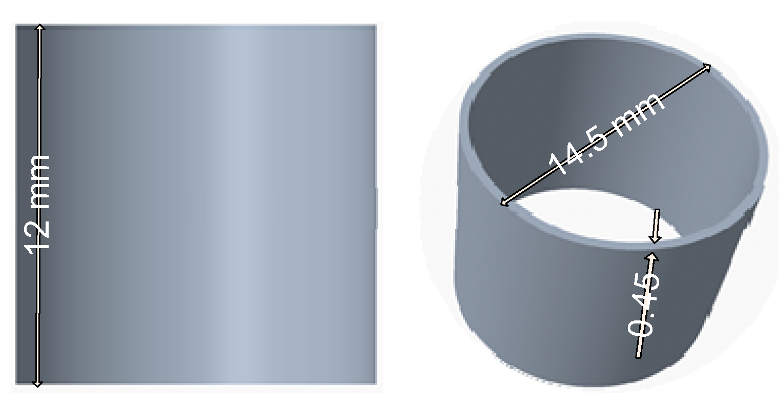
This research investigated the stability of the fused deposition modeling process through measuring the quality characteristics of the process outputs, namely FFF-printed products. A product should have some characteristics that are critical, and any deviations from these specifications beyond the specified limits can be expected to affect the primary function of the product. These characteristics are called critical-to-quality (CTQ). Quality characteristics are determined according to engineering and customer specifications. For this research, a cylinder product that has applications in many industries (e.g., automotive) was selected, as shown in Figure 1. In the considered product, the dimensional properties are considered as CTQ. Based on this, the three-dimensional properties of the products were measured, including the height, diameter, and wall thickness dimensions (see Figure 1). As the product under consideration possesses multiple CTQ characteristics, the correlations between these characteristics must be examined to determine whether univariate or multivariate process monitoring is appropriate.
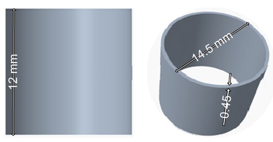
Figure 1.
Product design (CAD model).
2.1. Process
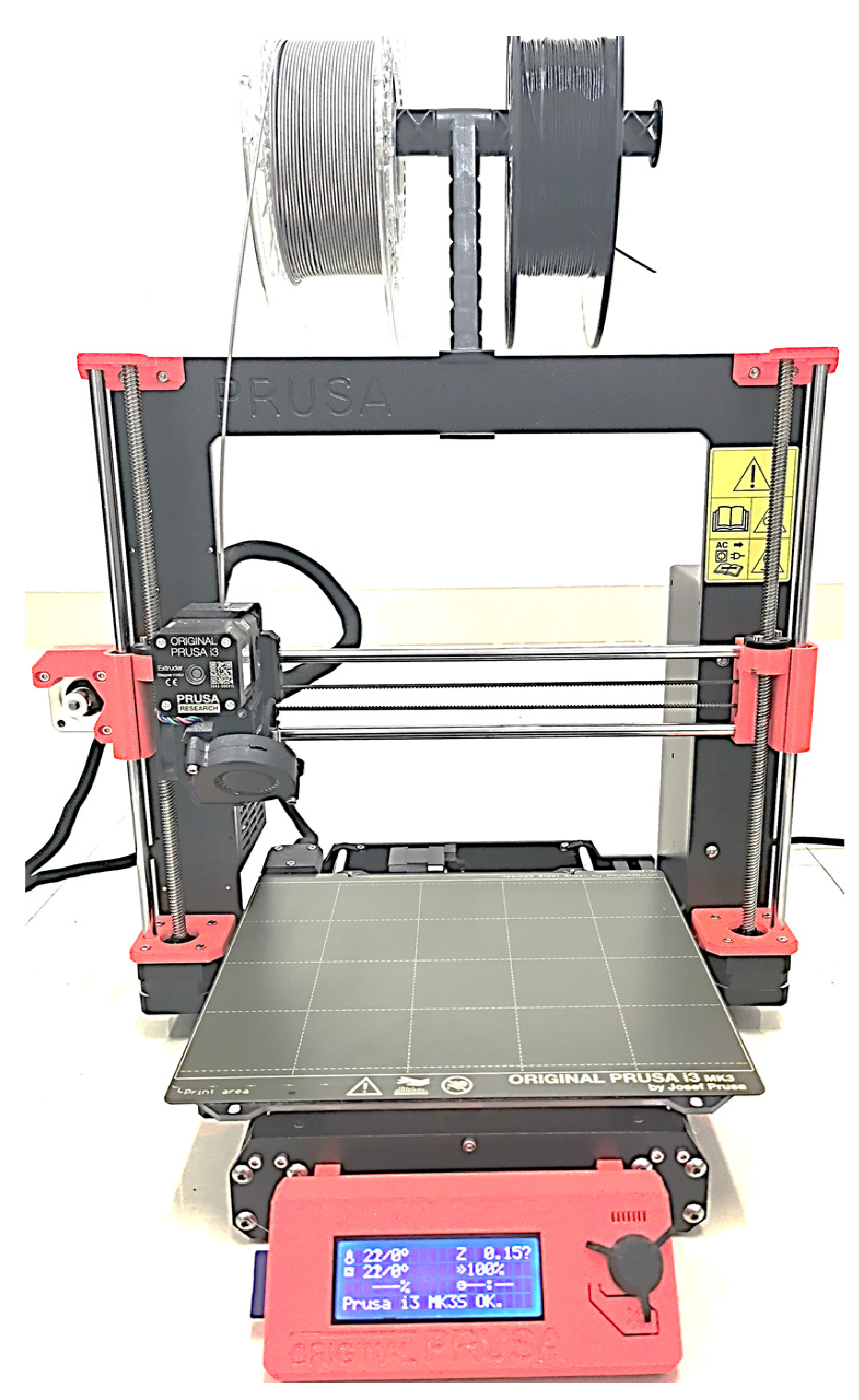
The product was designed using the CREO Parametric 8.0 software in STL format. The STL files of the designed samples were exported from the Creo 8.0 software and imported into Prusa Slicer 2.5.0 for slicing and G-code file generation. An open-access FFF printer (Original Prusa i3 MK3S+) equipped with a 0.4 mm nozzle diameter was used to manufacture the samples. The used printing parameters are listed in Table 1.

Table 1.
FFF printing parameters.
In FFF, a heating chamber is used to melt the polymer material, which is inserted into the system in the form of a filament. The extrusion pressure is created by the filament being pushed into the chamber by an arrangement resembling a tractor wheel; it is this pushing action that creates the pressure. The machine used in this study is shown in Figure 2.
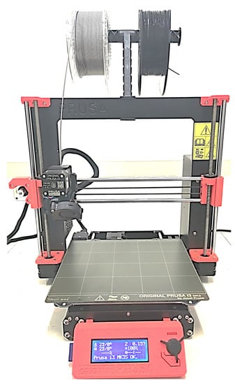
Figure 2.
FFF 3D printer.
2.2. Material
For this study, polylactic acid (PLA) polymer was used. The PLA filament (Prusament PLA Galaxy Silver filament) with a diameter of 1.75 mm was obtained from Prusa Polymers, Czech Republic. Polylactic acid (PLA) is popular for FFF printing due to its excellent printability, low cost, non-toxicity, biocompatibility, biodegradability, and eco-friendliness [36,37]. It shows a high tensile strength, modulus, and elongation at breakage [36]. PLA is an aliphatic polyester derived from non-fossil renewable resources such as corn and sugar cane [37]. In contrast, PLA has the lowest heat resistance of the major 3D printing polymers when it has not been annealed initially. Objects made of PLA can be created using techniques such as solvent welding, 3D printing, casting, injection molding, machining, and extrusion. PLA filament is designed for use in three-dimensional printing. When fabricating fused filament on desktop 3D printers, PLA may be utilized as a feedstock material. When used in a vapor chamber, the low boiling point of ethyl acetate makes it possible to smooth the surfaces of PLA.
3. Methodology
The special requirements of 3D-printed parts impose a high dimensional accuracy, which was considered in this study. In this context, we present a framework for monitoring the dimensional accuracy of FFF outputs, including specifying the critical quality characteristics, a data collection process, 3D printing, a measurement system, normality transformation, multivariate control chart optimization, and assessing the variability of the considered AM process. Moreover, there are many dimensional characteristics that are correlated with each other. Consequently, the proposed methodology is based on multivariate monitoring, which can take the correlations between QCs into consideration. The steps of the proposed methodology are listed in Table 2. The first two steps were described in the previous section, and are related to deciding which additive manufacturing process will be investigated. Determining the process and material to be used is crucial, as the later findings will only be valid with respect to these choices. Selecting the printed product, its characteristics, and applications will help in the trade-off process between the benefits and cost of highly accurate production.

Table 2.
Methodology steps.
3.1. Sampling and Printing Process
Sampling in the field of process monitoring is distinguished from other sampling methods in different scientific fields according to the data collection approach. Specifically, sampling involves two decisions that should be made in order to optimize the data collection and sampling process. These parameters are the sample size, which refers to how many parts should be collected and measured each time, and the frequency of collection, which denotes how often one should collect data or make a sample. A larger number of samples is better, but is not always economically ideal. In this regard, there should be a criterion to judge the appropriate number of samples, such as the average run length, which provides an indication of the point of time at which a process will go out of control. Regarding the sample size, in this context, it is well-known that the sample size typically varies between three and five [38]. Therefore, for this study, we considered ten samples with five observations in each sample. Three-dimensional printed parts are widely used in different industries. In this case, we designed a specific part that is commonly used as a joint in various automotive industries [39] (see Figure 1). This part has three critical dimension quality characteristics: diameter, height, and wall thickness. It is worth noting that the part was produced using a 3D printer that operates according to an FFF additive manufacturing process. The parts during printing and final products are shown in Figure 3.
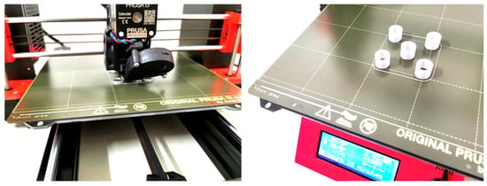
Figure 3.
Printing process.
3.2. Data Collection and Measurement Capability
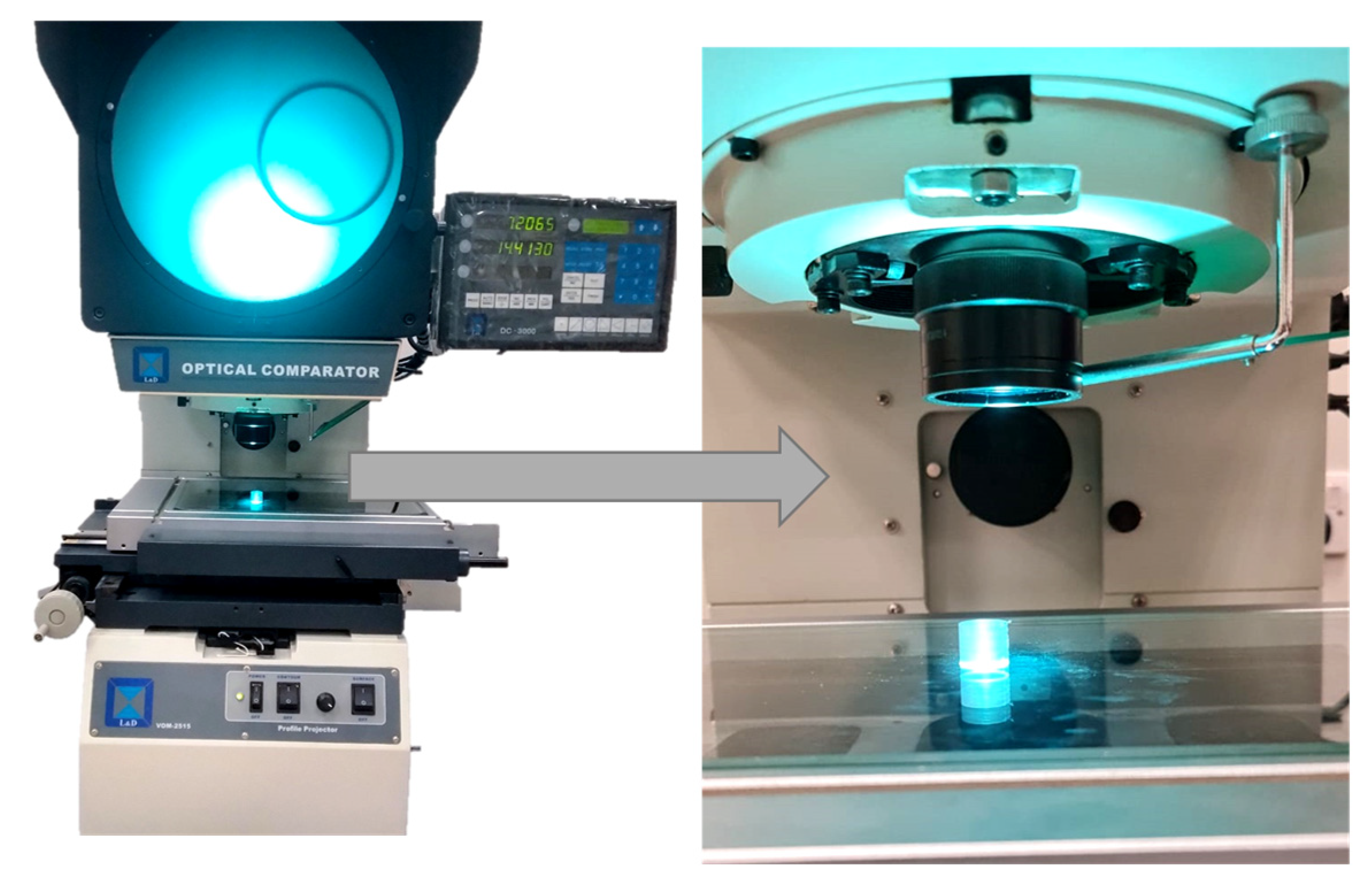
Furthermore, a data collection process was established to measure the three critical quality characteristics (i.e., diameter, height, and wall thickness). The measurement process was conducted using a very precise device called a profile projector, which is shown in Figure 4. The device model is Multi-Lens Profile Projector VOM-2515. According to the manufacture, the error of the contour measuring is under 0.08% under illumination. This measurement device was also examined for its capability to measure the same object various times consistently. Furthermore, the differences between operators were investigated. For this test, ten random parts were chosen to study the capability of the measurement system, where two different operators measured each of these ten parts twice.

Figure 4.
Profile projector measurement system.
3.3. Proposed Normality Improvement
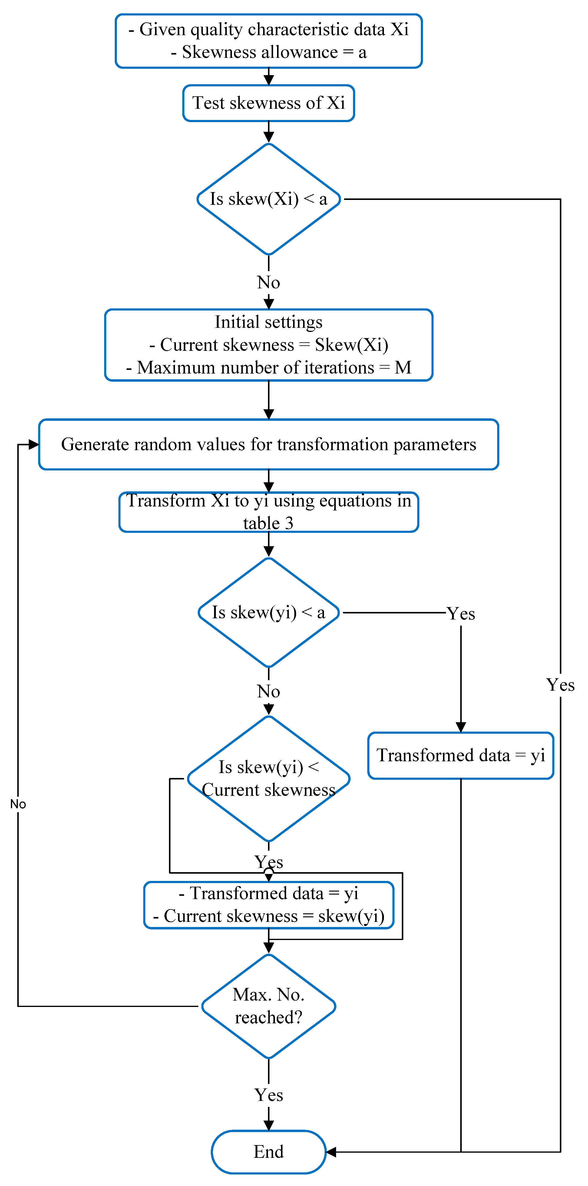
It is worth noting that most statistical tests are based on the assumption of normally distributed data; that is, the conclusion of such tests is valid only if the data fit the normal distribution. The normality assumption can be evaluated through the use of probability plots and histograms. Whenever the data are normally distributed, the measured characteristics may be examined for their correlation directly; otherwise, an appropriate transformation method should be used to transform the data. An improved Johnson transformation method can be used to transform the data to normality; basically, Table 3 was used to transfer the data to follow the normal distribution. However, this transformation does not always perform well. Therefore, another iterative search algorithm was used to continually change the transformation parameters until the data satisfied the normality test. The skewness of the data was used as a measure of the data normality, where normal data have a skewness of zero; a positive skewness indicates that the data are skewed to the right, whereas negative skewness indicates that the data are skewed to the left. The skewness has been used in the literature as an indication of data normality, such as in [40]. Thus, the algorithm presented in Figure 5 was used to search for the optimal parameters for the equations in Table 3, resulting in the minimal skewness of the considered data.

Table 3.
Johnson transformation system [41].
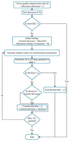
Figure 5.
The proposed transformation algorithm.
The correlations between different quality characteristics were investigated due to the associated direct effects on the process performance. The process under investigation was assessed using sample process outputs, where the outputs denote the finished products. The quality of a product is judged according to the characteristics that are required by the customer, and these characteristics are often statistically or functionally correlated. The existence of a correlation between different characteristics requires their joint monitoring and evaluation, as the individual evaluation of each characteristic may lead to wrong conclusions. A functional correlation is judged according to the engineering design and consumer requirements, whereas a statistical correlation should be tested using statistical methods. The correlation between two variables can be estimated using Equation (1), where the value of the correlation coefficient ranges from −1 to 1, indicating the strength and direction of the relationship between the two variables. A correlation coefficient of −1 between two variables implies a perfect negative relation (i.e., by increasing one variable, the other is decreased), whereas a correlation of 1 implies a perfect positive relation. The strength of the relationship varies from strong to weak as the correlation coefficient comes closer to zero.
where n is the sample size and xj and xk denote any two measured variables, such as height and diameter
3.4. Optimizing the Multivariate Process Variability Monitoring Chart
In this study, the multivariate exponential weighted moving average (MEWMA) chart proposed by Lowry, Cynthia A., et al. [42] was used to monitor the variability of the considered process. MEWMA was chosen due to its ability to detect small deviations in the process mean. MEWMA begins by computing a vector for each variable, as shown in Equation (2):
where n is the number of quality characteristics under investigation;
- λ is a constant number, and 0 < λ ≤ 1;
- z0 = μi;
- xi is the ith quality characteristics;
- zi is the MEWMA statistic; and μi is the mean of ith quality characteristics.
Then, the MEWMA chart gives an out-of-control signal and consequently indicates an unstable process if the following condition occurs:
where is estimated to be the value that results in a desired average run length (ARL), which is a method used to assess the choices made for the sample size and sampling frequency. ARL is the average number of points that should be drawn prior to a point showing an out-of-control situation. denotes the covariance matrix of :
where is the covariance matrix of . The covariance matrix Σ is computed for multivariate data , and i = 1,2,…n. In this study, i = 1, 2, and 3, for height, diameter, and wall thickness.
However, the MEWMA chart must be optimized by selecting the optimal chart parameters. The proposed methodology uses Monte Carlo simulation to optimize the MEWMA parameters, which involves optimizing the values of and that result in ARL = 370, which is a common ARL value used in the literature [38,43]. For example, p = 0.0027 is the probability that a point escapes beyond the limits of while the process is under control. As a result, when the process is under control, the ARL of the chart is ARL = 1/p = 1/0.0027 = 370.
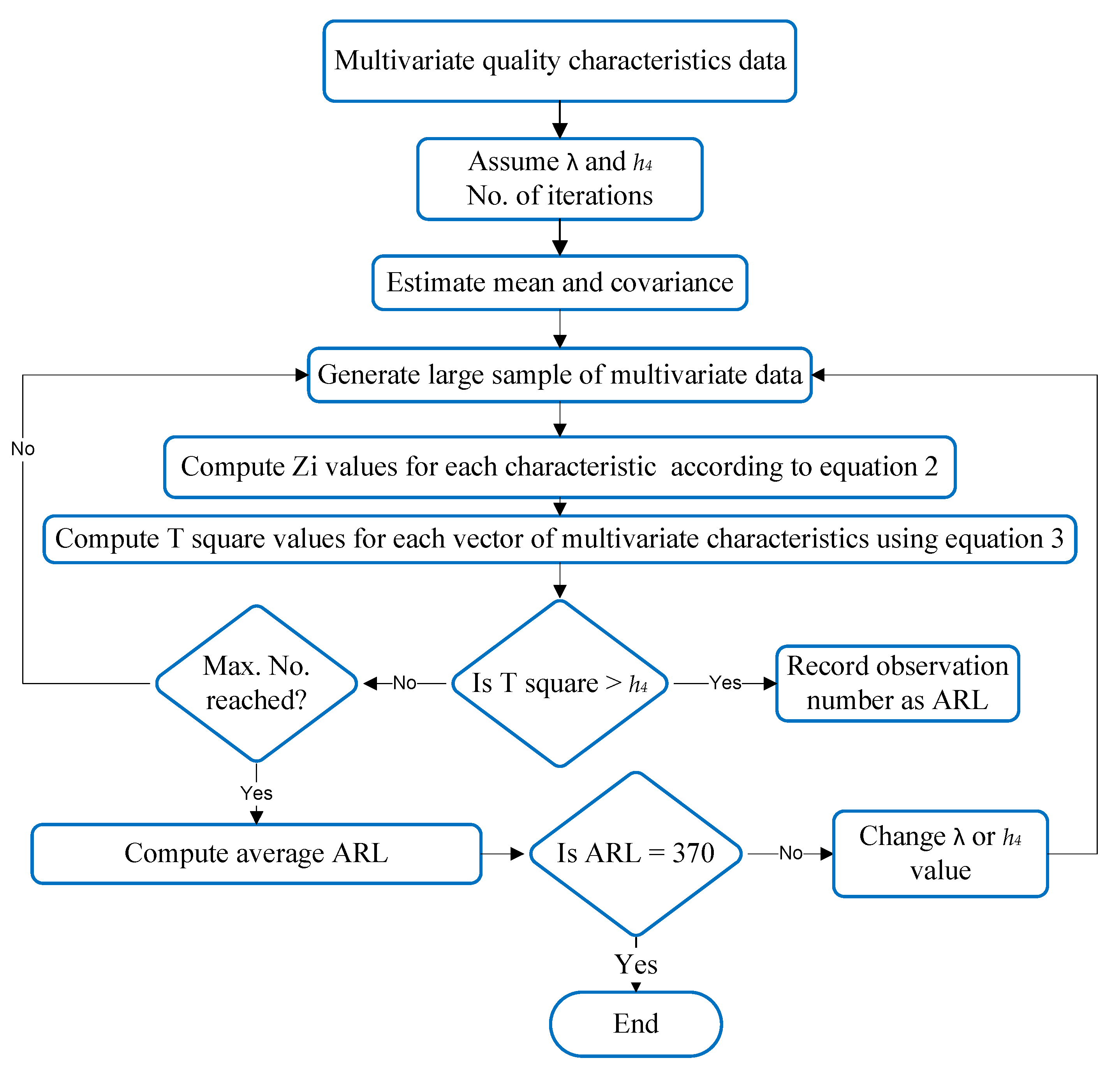
For this reason, an algorithm was constructed that iteratively searches for the optimal values of the MEWMA parameters. The proposed methodology is presented in Figure 6. The algorithm starts by obtaining the multivariate quality characteristic data. These data are then examined for normality, following which the multivariate data are normalized according to the equations provided in Table 3. When the data are normally distributed, the mean and covariance of the considered data are estimated in order to generate large multivariate data based on these parameters. The initial parameters of MEWMA are assigned to the algorithm to compute the corresponding MEWMA values , according to Equation (2). These values are then combined to form a single value for each vector, as in Equation (3). The values of are judged against the upper control limit h4. An initial value for the upper multivariate EWMA chart (h4) is suggested, which is further improved using the proposed MEWMA chart optimization algorithm. For a specific number of iterations, a large sample of multivariate characteristics is generated and evaluated against h4. Whenever an out-of-control signal is found, the corresponding observation number will be registered as an ARL. The process is continued until a preset number of iterations is met, following which the ARL is taken as the average ARL for all iterations. If the ARL is equal to 370, the algorithm is stopped and the optimal MEWMA parameters are obtained; otherwise, an action is taken by changing either or h4. Basically, different runs of the algorithm are performed with different values of h4: each time, a given value of h4 will be fixed, whereas is iteratively changed until ARL = 370 is satisfied.
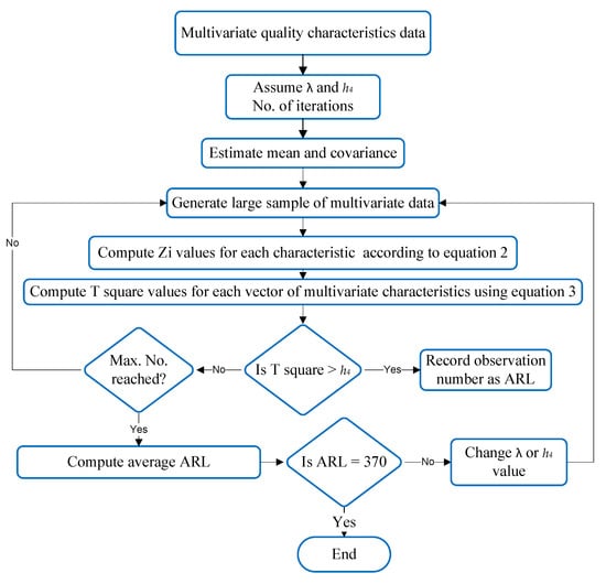
Figure 6.
Algorithm for optimizing MEWMA parameters.
4. Results and Discussions
4.1. Data Collection
The quality characteristics of the obtained samples were measured using a very precise device called a profile projector. Table 4 lists the measurement values. A total of ten samples were measured, each with a sample size of five. For this purpose, 50 parts were manufactured in batches of 5 in order to allow for the monitoring of the process using a sample size greater than one. Three quality characteristics were measured in each part, namely the height, diameter, and wall thickness of the manufactured parts. Consequently, a total of 150 measurements were taken using the profile projector.

Table 4.
Measurements of height, diameter, and wall thickness of 3D-printed parts.
4.2. Capability of the Measurement System
In any measurement system, it is necessary that the measurement system is accurate and precise. Accurate means that the measurement system measures correctly, whereas precise means that it gives the same measurement each time it is used for measuring the same object. However, it is useful to ensure the capability of the measurement system and that it is free of built-in errors or imprecisions using the gauge R&R method or repeatability and reproducibility measures. It is worth noting that there are generally variations from part to part associated with the manufacturing process. However, the measurement system may add more variations between parts if there are measurement errors. In this regard, the variation from part to part and gauge system variation may be considered good at values of around 10% and acceptable up to 30%. However, a variation greater than 30% is the maximum acceptable variability of the measurement system with respect to the tolerance of the process, such that corrective action should be taken [44].
Therefore, ten specimens were selected to be measured by three operators, where each operator measured each specimen twice. The measurements are presented in Table 5.

Table 5.
Measurement system variation test data.
The results of the gauge R&R test are provided in Table 6. The results indicate that the repeatability variation—which indicates the accuracy of the measurement device—was small (5.73%), and most of the measurement system variation was due to part-to-part deviations. The contribution of the measurement system variation to the total variation was 18% of the total variation, which includes the variations due to the measuring device (repeatability) and the variations among different operators (reproducibility).

Table 6.
Gauge R&R test results.
4.3. Normality Assumption
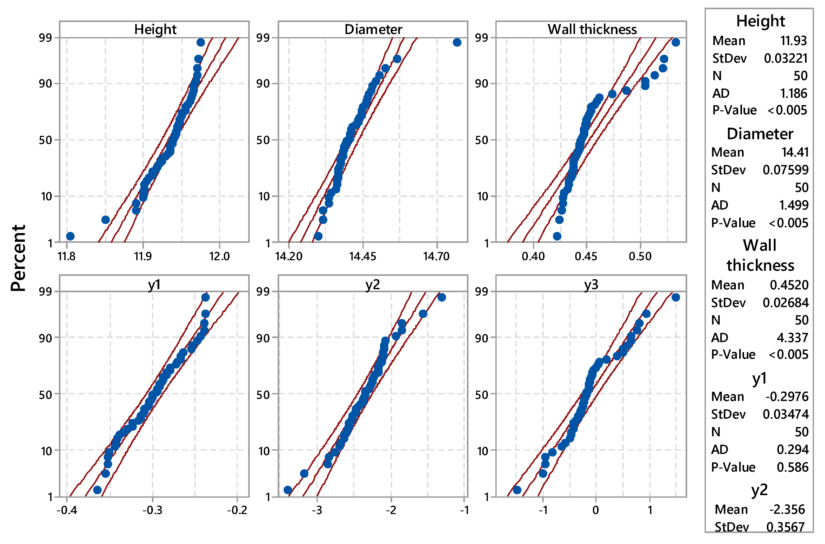
Next, the normality of the data was investigated. Figure 7 presents the normality plots for the weight, diameter, and wall thickness characteristics. Notably, the data for the three characteristics were not centered around a straight line. Furthermore, there were many outliers, especially in the wall thickness data, and the p-values corresponding to the three characteristics were all less than 0.05. These three indicators (off-center data, existence of outliers, and small p-values) all indicate a deviation in the data from the normal distribution. The , , and are the transformations of the three characteristics data, respectively. Figure 7 shows the improvement after the transformation using an improved Johnson transformation. The data become more centered around the straight line and the p-values increase.
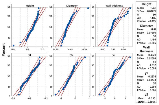
Figure 7.
Normality plots for height, wall thickness, and diameter characteristics.
Based on the results of the normality test, the transformation algorithm described in Figure 5 was used to transform the data to a normal distribution. For this purpose, a MATLAB code was developed to construct the suggested algorithm. The skewness was used as a measure of the accuracy of the transformation, or as a measure of the normality. As mentioned above, zero skewness indicates normal distribution, whereas positive and negative skewness indicate a right and left skew of the data, respectively. Table 7 shows the skewness results for the original, Johnson-transformed, and improved Johnson-transformed data. The results reveal that the Johnson transformation could reduce the absolute skewness of the data, whereas the iterative search further improved the skewness result. It is worth noting that negative and/or positive skewness can be further improved using the improved Johnson algorithm, whereas positively skewed data can be transformed by the Johnson transformation directly.

Table 7.
Skewness of the original and transformed data.
We used the MATLAB software to improve the quality of the transformation of the non-normal data, allowing it to become normally distributed. Consequently, the skewness of the transformed data was dramatically improved by designing an appropriate algorithm based on changing the parameters of the transformation function iteratively and evaluating the corresponding results against the original. Table 7 presents the skewness values for the considered three quality characteristics of the 3D-printed parts (height, ; diameter,; and wall thickness, ), with the skewness values of the same data after transformation by the two considered methods. The table clearly demonstrates the large differences between original and Johnson-/improved Johnson-transformed data in terms of skewness.
The correlation matrix between the three quality characteristics (height, diameter, and wall thickness) is presented in Table 8. The results indicate that the correlation between diameter and wall thickness was positive and moderate (r = 0.761). As there exists a correlation between the considered quality characteristics, these characteristics should be studied together in the multivariate analysis.

Table 8.
Correlation matrix.
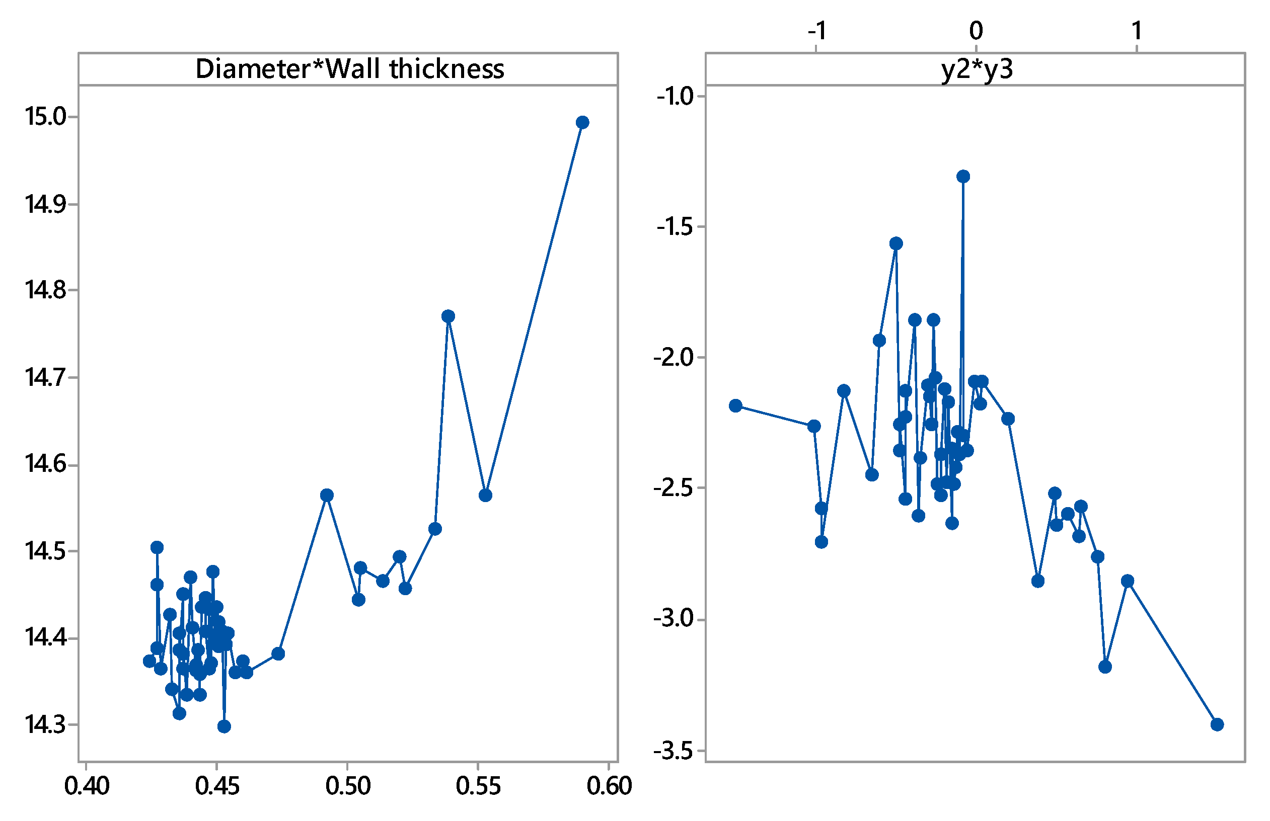
For the above analysis, a Pearson correlation test was conducted. This test requires the relationships between the investigated variables to be linear. Therefore, it is important to validate the linearity assumption. The scatter diagram is ideal for visualizing the type of relationship or judging the existence of a curvilinear relationship between two variables. The two quality characteristics (diameter, wall thickness, and their corresponding transformed data) were plotted in scatter diagrams to investigate the relationships between each pair, as shown in Figure 8 The graph shows a positive trend for diameter and wall thickness data, whereas a negative trend can be observed for the transformed data. Regarding the type of relationship, some constant linear patterns can be observed at the beginning of the data; however, a positive or negative linear pattern can be seen as the data values increase. The interpretation of the existing negative correlation between the transformed data, in contrast to the original data, is attributed to the transformation of each quality characteristic data separately using different parameters, especially when using an iterative search to further improve each type of transformed data.
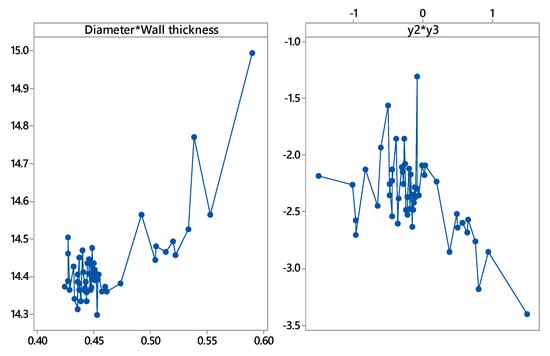
Figure 8.
Scatter diagram of diameter and wall thickness and their corresponding transformed data ( and ).
It is noticed that the most correlated values are those of high observations. This led to an investigation in this study to conduct an outlier test to ensure the existence of outlier values within the collected data. Table 9 shows the results of Grubbs’ test of outliers. The test revealed that, out of four tested variables, the diameter variable has one outlier value.

Table 9.
Grubbs’ test of outliers.
4.4. Multivariate Exponential Moving Average Chart
Constructing multivariate quality control charts begins with grouping all multivariate characteristics into a single factor. This is called dimension reduction, which is essential in establishing multivariate quality characteristics. Dimension reduction in the multivariate exponential moving average chart begins by using the equations mentioned earlier. After transforming the data to a normal distribution, each quality characteristic datum is transformed to an MEWMA statistic using Equation (3). Table 10 presents the mean and variance of original (x), transformed (y), and MEWMA statistic (z) data. The MEWMA statistic (z) data were obtained according to Equation (3), using a suggested value for . For the values presented in Table 10, the used value was 0.1. In fact, this is not a rule, and the choice of is subject to many considerations, such as the associated variability in the process and control limit. Therefore, this section details the optimization of MEWMA parameters, such as and h4.

Table 10.
Mean and variance of original (x), transformed (y), and standardized (z) data.
The multivariate exponential moving average chart parameters were optimized, where the best values of and control limits were chosen. is used to transform the data into standardized data. In addition, it is used in the formula for reducing the dimensionality of the multivariate data to a single factor. Its value ranges from zero to one. Each chosen value of results in a different optimal control limit (h4). The optimal control limit (h4) is chosen based on an average run length of 370. The reduced factor is used to monitor the variability of the process. To determine the variability of the considered additive manufacturing process, the mean and standard deviation of are used to generate large samples of normal data, which are evaluated against the control limit.
In this regard, a MATLAB code was designed to estimate the optimal control limit (h4) for data. The optimal limit is that which results in an ARL equal to 370 runs. In other words, the control limits that approximately cause the data to signal an out-of-control pattern are considered as optimal. It is worth noting that (and, consequently, the control limits) are based on choosing the value of ; that is, different values of result in different and different control limits.
For each combination of and h4, large samples were generated 1000 times, and the ARL was calculated for each iteration as shown in Table 11. The optimal ARL was set as 370 runs. The value of was first fixed, and the ARL was calculated for each value of h4. First, h4 was set as the value of the mean plus half of the standard deviation. With each iteration, h4 was increased by half of the standard deviation of the data, up to three standard deviations. Changing has no significant effect on the ARL value; however, different values of h4 led to different ARL values, with the ARL increasing exponentially along with an increase in h4.

Table 11.
ARL values under different MEWMA parameters.
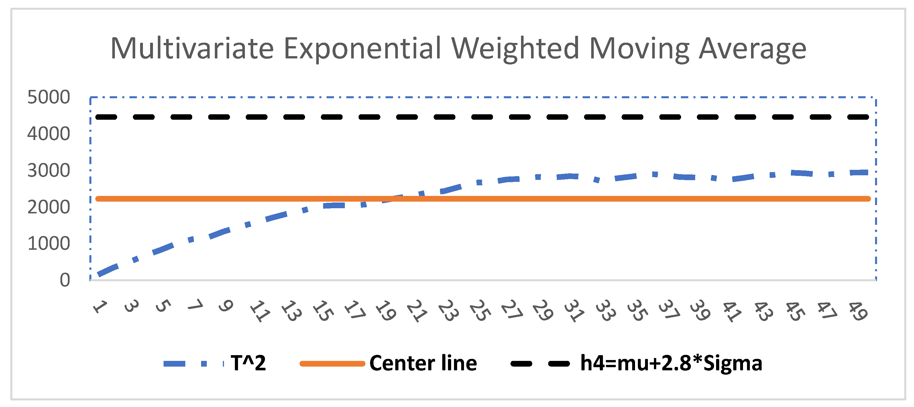
The optimization of the MEWMA parameters revealed that the considered additive manufacturing process was relatively stable. In particular, the natural tolerance (the mean plus three standard deviations) revealed an ARL larger than 370 runs. This indicates that this process will present an out-of-control signal after 370 runs when h4 is set to the mean plus 2.8 standard deviations. To illustrate the stability of the process, Figure 9 shows the control chart of the process. Clearly, the plotted means are far from the control limit (h4). However, the chart in Figure 9 also shows an increasing trend in the beginning of the chart; this is due to the nature of the chart calculations, which start with very small data and move toward the center line before showing stability. Stability is indicated by the points after crossing the center line, which are plotted horizontally. As the increase in the plotted data reduces, the process is predicted to be in control when more samples have been plotted.
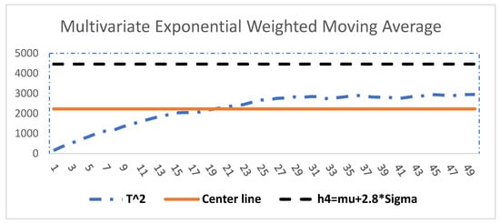
Figure 9.
Optimized MEWMA control chart.
5. Conclusions
AM processes are widely applied in different real-life applications to manufacture various products that must possess high-quality characteristics and precise dimensions. To achieve this goal, AM processes should be monitored using appropriate methods, such as the approach proposed in this paper. An effective monitoring process starts by focusing on the critical-to-quality characteristics, which are obtained according to customer requirements and engineering designs. When a product has more than one QC, they should be monitored jointly when they are statistically and/or functionally correlated. Practically, the data of different characteristics of a single product may be reduced to one index, which can then be used to monitor the stability of the considered AM process. It is worth noting that most real industry data are not normally distributed. Therefore, we presented an improved Johnson transformation algorithm. This proposed algorithm is based on optimizing the Johnson transformation with respect to the objective of minimizing the absolute value of the skewness of the data. When transforming the data, improving the skewness of the data has been recommended as an effective measure of normality. Moreover, the literature has suggested using a profiler projector to measure the considered dimensions, which was evaluated using a gauge R&R test and was shown to be capable of reliably repeating the same measurement. Finally, we investigated choosing the appropriate multivariate chart to monitor the considered process in terms of optimizing the chart parameters against the average run length. As a result, we proposed a heuristic optimization algorithm, which was implemented using MATLAB to simulate the process under different parameters. The optimized parameters were the values of the MEWMA chart constant and the upper control limit (h4). Generally, the values of the MEWMA chart constant ranged between 0 and 1, while the upper control limit (h4) was set to be in the range of the mean plus 0.5–3 standard deviations (σ) of the process. Simulation codes were run to generate very large replicate samples to evaluate the ARL against each configuration of the chart parameters.
Moreover, this work suggests future research directions to be investigated. Some of these directions evaluate the FFF process in term of engineering specifications. An evaluation of the AM process could be conducted using the process’s outputs against specifications. Process capability analysis is one of the quality tools that can be used to evaluate the capability of the process to meet the desired specification limits. Using process capability indices for multivariate AM processes’ responses or quality characteristics is a promising research direction. In addition, multi-response optimization using quality characteristics is another research direction. Each AM process has many parameters that can be changed to influence the different responses of the process. Studying curves of different responses simultaneously is expected to reveal important findings. The multiple responses can be treated together by using multivariate process capability indices. This work can also be applied to more complex scenes, such as corners, 3D lattices, and geometrical cylindricity to figure out the dimensional accuracy with different designs. Moreover, the measurement system is another research point. In this context, various measurement systems can be compared. In addition, analyzing the repeatability of the measure can be extended to involve more than two operators.
Author Contributions
Conceptualization, M.A. and A.M.A.-A.; methodology, M.A. and A.Y.A.; software, M.A.; validation, A.M.A.-A., A.Y.A. and M.S.; formal analysis, M.A.; investigation, M.A.; resources, M.S.; data curation, M.A.; writing—original draft preparation, M.A.; writing—review and editing, A.Y.A.; visualization, M.A.; supervision, A.M.A.-A. and A.Y.A.; project administration, A.M.A.-A. and A.Y.A.; funding acquisition, A.M.A.-A. and A.Y.A. All authors have read and agreed to the published version of the manuscript.
Funding
This research was funded by King Saud University through Researchers Supporting Project number (RSP2023R256), King Saud University, Riyadh, Saudi Arabia.
Data Availability Statement
The data presented in this study are available in this article.
Acknowledgments
The authors are thankful to King Saud University for funding this work through Researchers Supporting Project number (RSP2023R256), King Saud University, Riyadh, Saudi Arabia.
Conflicts of Interest
The authors declare no conflict of interest.
References
- Javaid, M.; Haleem, A.; Singh, R.P.; Suman, R.; Rab, S. Role of additive manufacturing applications towards environmental sustainability. Adv. Ind. Eng. Polym. Res. 2021, 4, 312–322. [Google Scholar] [CrossRef]
- Ngo, T.D.; Kashani, A.; Imbalzano, G.; Nguyen, K.T.; Hui, D. Additive manufacturing (3D printing): A review of materials, methods, applications and challenges. Compos. Part B Eng. 2018, 143, 172–196. [Google Scholar] [CrossRef]
- Pham, D.T.; Gault, R.S. A comparison of rapid prototyping technologies. Int. J. Mach. Tools Manuf. 1998, 38, 1257–1287. [Google Scholar] [CrossRef]
- Kruth, J.-P. Material incress manufacturing by rapid prototyping techniques. CIRP Ann. 1991, 40, 603–614. [Google Scholar] [CrossRef]
- Liu, Z.; Wang, Y.; Wu, B.; Cui, C.; Guo, Y.; Yan, C. A critical review of fused deposition modeling 3D printing technology in manufacturing polylactic acid parts. Int. J. Adv. Manuf. Technol. 2019, 102, 2877–2889. [Google Scholar] [CrossRef]
- Stratasys. Fused Deposition Modelling. Available online: http://www.stratasys.com (accessed on 16 November 2022).
- Ian Gibson, I.G. Additive Manufacturing Technologies 3D Printing, Rapid Prototyping, and Direct Digital Manufacturing; Springer: Berlin/Heidelberg, Germany, 2015. [Google Scholar]
- Ligon, S.C.; Liska, R.; Stampfl, J.; Gurr, M.; Mülhaupt, R. Polymers for 3D printing and customized additive manufacturing. Chem. Rev. 2017, 117, 10212–10290. [Google Scholar] [CrossRef] [PubMed]
- Monticeli, F.; Neves, R.; Ornaghi, H., Jr.; Almeida, J., Jr. Prediction of Bending Properties for 3D-Printed Carbon Fibre/Epoxy Composites with Several Processing Parameters Using ANN and Statistical Methods. Polymers 2022, 14, 3668. [Google Scholar] [CrossRef]
- Ciotti, M.; Campana, G.; Mele, M. A review of the accuracy of thermoplastic polymeric parts fabricated by additive manufacturing. Rapid Prototyp. J. 2022, 28, 358–389. [Google Scholar]
- Turner, B.N.; Strong, R.; Gold, S.A. A review of melt extrusion additive manufacturing processes: I. Process design and modeling. Rapid Prototyp. J. 2014, 20, 192–204. [Google Scholar] [CrossRef]
- Bellini, A.; Güçeri, S.; Bertoldi, M. Liquefier dynamics in fused deposition. J. Manuf. Sci. Eng. 2004, 126, 237–246. [Google Scholar] [CrossRef]
- Agarwala, M.K.; Jamalabad, V.R.; Langrana, N.A.; Safari, A.; Whalen, P.J.; Danforth, S.C. Structural quality of parts processed by fused deposition. Rapid Prototyp. J. 1996, 2, 4–19. [Google Scholar] [CrossRef]
- Idà, E.; Nanetti, F.; Mottola, G. An Alternative Parallel Mechanism for Horizontal Positioning of a Nozzle in an FDM 3D Printer. Machines 2022, 10, 542. [Google Scholar] [CrossRef]
- Kim, H.; Lin, Y.; Tseng, T.-L.B. A review on quality control in additive manufacturing. Rapid Prototyp. J. 2018, 24, 645–669. [Google Scholar] [CrossRef]
- Everton, S.K.; Hirsch, M.; Stravroulakis, P.; Leach, R.K.; Clare, A.T. Review of in-situ process monitoring and in-situ metrology for metal additive manufacturing. Mater. Des. 2016, 95, 431–445. [Google Scholar] [CrossRef]
- Foster, B.; Reutzel, E.; Nassar, A.; Hall, B.; Brown, S.; Dickman, C. Optical, layerwise monitoring of powder bed fusion. In 2014 International Solid Freeform Fabrication Symposium; University of Texas at Austin: Austin, TX, USA, 2015. [Google Scholar]
- Barrett, C.; Carradero, C.; Harris, E.; Rogers, K.; MacDonald, E.; Conner, B. Statistical analysis of spatter velocity with high-speed stereovision in laser powder bed fusion. Prog. Addit. Manuf. 2019, 4, 423–430. [Google Scholar] [CrossRef]
- Ablat, M.A.; Qattawi, A. Numerical simulation of sheet metal forming: A review. Int. J. Adv. Manuf. Technol. 2017, 89, 1235–1250. [Google Scholar] [CrossRef]
- Bandyopadhyay, A.; Traxel, K.D. Invited review article: Metal-additive manufacturing—Modeling strategies for application-optimized designs. Addit. Manuf. 2018, 22, 758–774. [Google Scholar] [CrossRef]
- Colosimo, B.M.; Huang, Q.; Dasgupta, T.; Tsung, F. Opportunities and challenges of quality engineering for additive manufacturing. J. Qual. Technol. 2018, 50, 233–252. [Google Scholar] [CrossRef]
- Colosimo, B.M.; Grasso, M. Spatially weighted PCA for monitoring video image data with application to additive manufacturing. J. Qual. Technol. 2018, 50, 391–417. [Google Scholar] [CrossRef]
- Iqbal, A.; Mahmood, T.; Ali, Z.; Riaz, M. On Enhanced GLM-Based Monitoring: An Application to Additive Manufacturing Process. Symmetry 2022, 14, 122. [Google Scholar] [CrossRef]
- Luan, H.; Post, B.K.; Huang, Q. Statistical process control of in-plane shape deformation for additive manufacturing. In Proceedings of the 2017 13th IEEE Conference on Automation Science and Engineering (CASE), Xi’an, China, 20–23 August 2017; pp. 1274–1279. [Google Scholar]
- Budzik, G.; Woźniak, J.; Paszkiewicz, A.; Przeszłowski, Ł.; Dziubek, T.; Dębski, M. Methodology for the quality control process of additive manufacturing products made of polymer materials. Materials 2021, 14, 2202. [Google Scholar] [CrossRef]
- Khanzadeh, M.; Tian, W.; Yadollahi, A.; Doude, H.R.; Tschopp, M.A.; Bian, L. Dual process monitoring of metal-based additive manufacturing using tensor decomposition of thermal image streams. Addit. Manuf. 2018, 23, 443–456. [Google Scholar] [CrossRef]
- Kousiatza, C.; Karalekas, D. In-situ monitoring of strain and temperature distributions during fused deposition modeling process. Mater. Des. 2016, 97, 400–406. [Google Scholar] [CrossRef]
- Zhang, S.; He, K.; Cabrera, D.; Li, C.; Bai, Y.; Long, J. Transmission condition monitoring of 3d printers based on the echo state network. Appl. Sci. 2019, 9, 3058. [Google Scholar] [CrossRef]
- Oleff, A.; Küster, B.; Stonis, M.; Overmeyer, L. Process monitoring for material extrusion additive manufacturing: A state-of-the-art review. Prog. Addit. Manuf. 2021, 6, 705–730. [Google Scholar] [CrossRef]
- Gomathi, K.; Ganesh, T.; Bharanidharan, J.; Prajathkar, A.A.; Aravinthan, R. Condition Monitoring of 3D Printer Using Micro Accelerometer. In IOP Conference Series: Materials Science and Engineering, Proceedings of the International Virtual Conference on Robotics, Automation, Intelligent Systems and Energy (IVC RAISE 2020), Erode, India, 15 December 2020; IOP Publishing: Bristol, UK, 2021; Volume 1055, p. 012035. [Google Scholar]
- Vidakis, N.; David, C.; Petousis, M.; Sagris, D.; Mountakis, N. Optimization of key quality indicators in material extrusion 3D printing of acrylonitrile butadiene styrene: The impact of critical process control parameters on the surface roughness, dimensional accuracy, and porosity. Mater. Today Commun. 2023, 34, 105171. [Google Scholar] [CrossRef]
- Leng, S.; McGee, K.; Morris, J.; Alexander, A.; Kuhlmann, J.; Vrieze, T.; McCollough, C.H.; Matsumoto, J. Anatomic modeling using 3D printing: Quality assurance and optimization. 3d Print. Med. 2017, 3, 6. [Google Scholar] [CrossRef]
- Mahmood, S.; Qureshi, A.; Talamona, D. Taguchi based process optimization for dimension and tolerance control for fused deposition modelling. Addit. Manuf. 2018, 21, 183–190. [Google Scholar] [CrossRef]
- Kumar, S.; Kolekar, T.; Patil, S.; Bongale, A.; Kotecha, K.; Zaguia, A.; Prakash, C. A low-cost multi-sensor data acquisition system for fault detection in fused deposition modelling. Sensors 2022, 22, 517. [Google Scholar] [CrossRef]
- Alatefi, M.; Ahmad, S.; Alkahtani, M. Performance evaluation using multivariate non-normal process capability. Processes 2019, 7, 833. [Google Scholar] [CrossRef]
- Diez-Escudero, A.; Andersson, B.; Persson, C.; Hailer, N.P. Hexagonal pore geometry and the presence of hydroxyapatite enhance deposition of mineralized bone matrix on additively manufactured polylactic acid scaffolds. Mater. Sci. Eng. C 2021, 125, 112091. [Google Scholar] [CrossRef] [PubMed]
- Bardot, M.; Schulz, M.D. Biodegradable poly (Lactic acid) nanocomposites for fused deposition modeling 3d printing. Nanomaterials 2020, 10, 2567. [Google Scholar] [CrossRef] [PubMed]
- Montgomery, D.C. Introduction to Statistical Quality Control; John Wiley & Sons: Hoboken, NJ, USA, 2020. [Google Scholar]
- Udroiu, R.; Braga, I.C. System performance and process capability in additive manufacturing: Quality control for polymer jetting. Polymers 2020, 12, 1292. [Google Scholar] [CrossRef] [PubMed]
- Abbasi, B.; Akhavan Niaki, S.T. Estimating process capability indices of multivariate nonnormal processes. Int. J. Adv. Manuf. Technol. 2010, 50, 823–830. [Google Scholar] [CrossRef]
- Johnson, N. Systems Of Frequency Curves Generated By Methods Of Translation. Biometrika 1949, 36, 149–176. [Google Scholar] [CrossRef]
- Lowry, C.A.; Woodall, W.H.; Champ, C.W.; Rigdon, S.E. A multivariate exponentially weighted moving average control chart. Technometrics 1992, 34, 46–53. [Google Scholar] [CrossRef]
- Gunaratne, N.G.T.; Abdollahian, M.A.; Huda, S.; Yearwood, J. Exponentially weighted control charts to monitor multivariate process variability for high dimensions. Int. J. Prod. Res. 2017, 55, 4948–4962. [Google Scholar] [CrossRef]
- Beckert, S.F.; Paim, W.S. Critical analysis of the acceptance criteria used in measurement systems evaluation. Int. J. Metrol. Qual. Eng. 2017, 8, 23. [Google Scholar] [CrossRef]
Disclaimer/Publisher’s Note: The statements, opinions and data contained in all publications are solely those of the individual author(s) and contributor(s) and not of MDPI and/or the editor(s). MDPI and/or the editor(s) disclaim responsibility for any injury to people or property resulting from any ideas, methods, instructions or products referred to in the content. |
© 2023 by the authors. Licensee MDPI, Basel, Switzerland. This article is an open access article distributed under the terms and conditions of the Creative Commons Attribution (CC BY) license (https://creativecommons.org/licenses/by/4.0/).

