Economic Dispatch of Combined Heat and Power Plant Units within Energy Network Integrated with Wind Power Plant

Abstract

Cogeneration, also known as a combined heat and power (CHP) system, produces both power and heat simultaneously. It reduces the operating costs and emissions by utilising waste heat from steam turbines and contributes to incapacitating the intermittency of renewable energy. The CHP-economic dispatch (CHP-ED) is needed to overcome the load dynamics as well as renewable intermittency. In this work, a CHP system connected with a wind power plant is considered for analysing the CHPED within a typical power system area. This study examines, the CHPED with and without a wind integrated energy network. The main objective of this work is to minimise the total operating cost, while meeting the generators’ constraints and prioritising the wind power output. The feasible operating region, valve point loading impact, and prohibited working regions of the CHP plants are taken while finding a CHPED solution with an integrated wind turbine. To find a CHPED solution, an optimisation algorithm was applied and the algorithm was based on selecting the best and worst scenarios. A typical 48-unit structure was used for validating the considered technique’s success for CHPED with/without a wind power plant. In our investigation, we found that operational costs were significantly reduced with a wind energy system. The presented methodology will be useful for the CHPED process of the decentralised CHP units for promoting further integration of the wind turbines and other distributed clean energy resources.

1. Introduction

Power generation from conventional thermal power plants has become less attractive in recent years. It decreases the productivity of a traditional power plant and increases the pollutant gases in the environment [1]. Due to the increasing demand for electricity consumption, cogeneration plants are becoming more popular. A cogeneration, i.e., combined heat and power (CHP), system increases the overall combined efficiency up to 90% and reduces the emissions by 13–18% [2]. The CHP units are more economical for operating in a power system, because they contribute in electrical and thermal energy at the same time [3]; and can facilitate the integration of intermittent renewable energy sources due to their capability of fast power dispatching as well as for primary frequency control. The economic dispatch (ED) operation is critical in optimising the power flows power system operation, especially with increasing penetration of renewable resources. The objective of ED is to reduce the cost of fuel while meeting all the network constraints [4].

The integration of CHP units with traditional ED problems has resulted in a significant change in the power sector. In terms of economics and environmental impact, cogeneration units are a better alternative in the power sector [5]. The operating performance of energy network with thermal power plants is very complex. It creates nonlinear and nonconvex behaviours, and generate technical operational challenges with renewable energy sources [6]. However, a sinusoidal term is considered with the fuel cost function to address the valve point loading (VPL) effect of thermal units. It pushes the objective function into a nonconvex region. For a better understanding, the feasible operating region and network losses should be considered [7].

Several mathematical and metaheuristic optimisation methods have been introduced in recent decades. Mathematical optimisation includes Newton’s method [8], Lagrange relaxation [9], Lagrange relaxation with a surrogate subgradient technique [10], the branch-and-bound algorithm [11], and so on. The disadvantages of the above methods are that they are not suitable for nonconvex and nonlinear objective problems.

However, metaheuristic techniques overcome the aforementioned problem and are able to handle both single- and multiobjective problems. The single-objective function consists of minimising operational costs. In [12], the author(s) suggested an IGA-MU by adjusting the penalty value to obtain a small population size. In contrast, in [13], a modified genetic algorithm with a penalty function method was used to resolve the CHPED problem. A self-adaptive genetic algorithm was introduced in [14], based on selection and crossover phenomena with good convergence characteristics. In [15], the hybrid combination of genetic harmony searching was proposed to resolve the CHPED issue. In [16], the authors suggested the binary value technique, which removes the nonconvexity of the CHPED issue. However, the VPL and POZs of power units were not taken into consideration in the articles [12,13,14,15,16] and CHPED with the plant’s constraints with the integration of a wind power plant was not sufficiently analysed in the literature.

In [17], the hybridisation of DE (differential evolution)-SQP (sequential quadratic programming) was applied to minimise the fuel price and pollutants, while taking the ramp rate limits into consideration. The algorithm gave effective results. Similarly, in [18], a novel self-adaptive learning technique was used to explain CHP-ED optimisation, where VPL, the ramp rate limit, and the reserve constraint were considered. An demand incentive based technique was adopted to minimise the fuel price and carbon emissions [19]. In [20], the authors suggested the CSA to solve the CHP-ED issue and it is easy to implement due to less design parameters. In [21], the Lagrangian alternative technique was applied to replace the nonconvex region by a convex operating zone by using the Big M theory.

In [22], PSO with a time varying acceleration coefficient (TVAC-PSO) optimisation procedure was applied. The dynamic alteration of the coefficient generated the optimal search space and removed early convergence. In contrast, the oppositional teacher–learner-based (OTLBO) method improved the CHPED solution’s accuracy and demonstrated fast convergence in [23]. In [24], the authors recommended a crisscross optimisation algorithm using horizontal and vertical crossover to solve CHPED effectively. Meanwhile, in [25], a genetic algorithm with real coding (RCGA) method was applied to the standard system using advanced alteration to explain CHPED, including VPL and power losses.

The intermittent behaviour of the thermal units due to POZs, creates some practical operational challenges in the system. The authors have proposed the oppositional group searching method to explain CHPED problem considering POZs and VPL [26]. Another proposed method for addressing the CHPED challenge is the heat exchange algorithm, which consists of diffusion, condensation, and radiation [27]. To overcome the CHPED problem with large barriers, a biogeography based PSO was developed, which employs a migrant agent to ensure the desired particle orientation [28].

Several authors have proposed a multi-objective function which consists of minimising fuel costs and emissions. In [29], a PSO with time-varying coefficients (TVAC-PSO) was proposed to solve CHP economic/emission dispatching including losses. In [30], the author proposed different metaheuristic algorithms to resolve the CHPED problem consisting of VPL and transmission losses. To increase the solution’s accuracy, other multi-objective solvers with different weighting factors were used. The NSGA-II algorithm was applied in [31] to solve the CHPED problem.

Each of the above-mentioned activities can become more cost-effective when decentralised forms of clean energies (e.g., a wind power plant) are combined with CHP structures. In this article, a wind energy system is integrated with the CHPED framework. Combining a CHP with a wind energy system is the most efficient mode to transition to a zero-carbon future, while also reducing the operating fuel costs. The most challenging aspect of incorporating wind power into the CHPED is the unpredictability of wind speed [32]. Large-scale wind energy integration needs power system operational adaptability to manage the supply and demand imbalances. The CHP system can effectively contribute in managing the variability of wind energy resources and contributes in operational flexibility within power system due to its fast power-dispatching capability [33].

Several research studies have been carried out in the field of basic economic dispatch problems with renewable sources. For example, in [34], the author developed a decomposition-based differential evolution (DE) technique for electric/thermal allocation using stochastic wind, photovoltaic, and hydroelectric power. The researcher proposed a new EED combined with wind energy to begin investigating the carbon tax [35]. The overall objective of developing such an alternative is to reduce the operational fuel cost and to promote the penetration of renewables. The DE technique could be used to evaluate the optimal power flow (OPF) based on decentralised energy resources [36]. Probability density features are frequently used to forecast renewable energy outcomes. Many sustainable economic load dispatch discussions take place to ensure low costs and carbon emissions [37,38]. In [39], the author(s) proposed the PSO to resolve a combined economic/emission scheduling issue involving various power generation modules and photovoltaics.

Earlier, wind based CHPED problem has not been addressed significantly considering the CHP unit constraints [34,35,36,37,38,39]. Therefore, this article proposes use of an optimisation algorithm for CHPED, with and without wind power plant integrated in energy network. The operational constraints of a CHP unit with the prioritisation of wind energy are used in the algorithm for finding the wind-based CHPED (W-CHPED). The other optimisation techniques, previously discussed, are difficult to apply due to the considered constraints/operating variables. The proper tuning of these variables creates complications during programming, so a very simple metaphor-less Rao-3 algorithm is proposed to handle the constrained CHPED/W-CHPED issue. This is based on best- and worst-case scenarios. A random communication occurs between the particles and it only needs two design variables i.e., population size and number of iterations. In this work or more accurate analysis, VPL, the POZs of power plants, and the feasible operating regions (FOR) of CHP units are taken into consideration. To handle all the constraints, the external penalty technique is applied. A typical 48-unit test case power system network is used to authenticate the success of the planned procedure. The outcomes demonstrate that when a wind energy system is integrated with a CHPED structure, the operational fuel cost is significantly reduced.

The rest of the paper is structured as follows: The mathematical design of the wind-based CHPED system is provided in Section 2. The suggested Rao-3 algorithm is given in Section 3. Section 4 compares the results of the considered 48-unit test case system. Finally, in Section 5, the obtained results and findings are concluded.

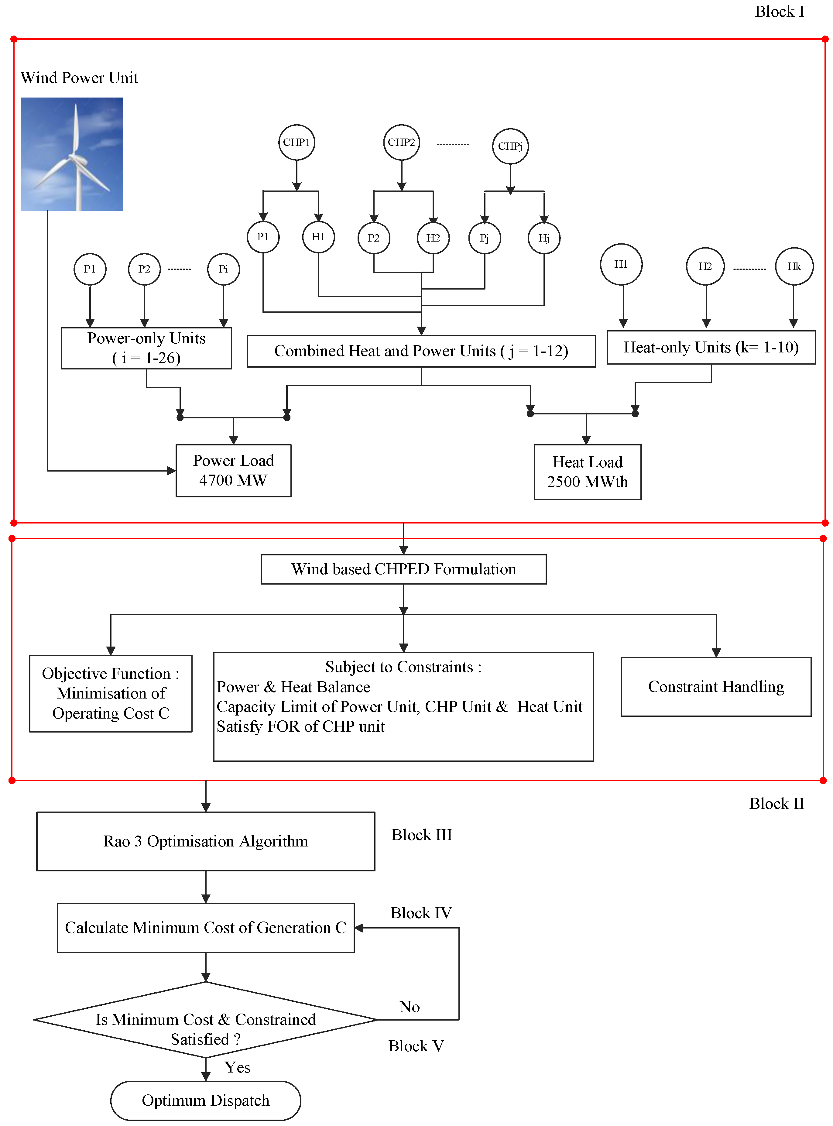
2. Mathematical Modelling of Wind-CHPED

The cost functions of various units are included in the statistical model of the wind-based CHPED issue.

2.1. Thermal Power Plant Costing

The power unit’s fuel analytical function is represented via a quadratic polynomial and given by Equation (1) [40,41].

$$\sum _{i=1}^{N_T}{C}_i(P_i^T)=\sum _{i=1}^{N_T}[a_i{P}_i^{T^2}+b_i{P}_i^T+c_i](\$/h)$$

(1)

In Equation (1), for an ${\mathrm{i}}^{\mathrm{t}\mathrm{h}}$ thermal power plant, $C_i(P_i^T)$ is the fuel cost, ${\mathrm{P}}_{\mathrm{i}}^{\mathrm{T}}$ is the power output, N_T is the number of thermal power plant units, and $a_i,b_i\mathrm{a}\mathrm{n}\mathrm{d}{c}_i$ are the cost constants.

Due to valve point loading impacts, the optimisation function converts into a nonconvex zone. It causes ripples in the heat rate characteristics. A rectified sine wave component is inserted to the cost function for realistic modelling [40,41]. Equation (2) represents a mathematical concept for a cost function with valve point loading.

$$\sum _{i=1}^{N_T}{C}_i(P_i^T)=\sum _{i=1}^{N_T}[a_i{P}_i^{T^2}+b_i{P}_i^T+c_i+|e_{i}sin\{f_i\left(P_i^{T^{min}}-P_i^T\right)\}|](\$/h)$$

(2)

In Equation (2) for the $i^{th}$ unit, $e_i$ and $f_i$ are cost constants, and $P_i^{T^{min}}$ is the minimum power.

2.2. Cogeneration Unit Costing

The analytical cost function for the cogeneration unit is given in Equation (3) [42,43,44].

$$\sum _{j=1}^{N_C}{C}_j\left(P_j^C,h_j^C\right)=\sum _{j=1}^{N_C}[a_j{P}_j^{C^2}+b_j{P}_j^C+c_j+d_j{h}_j^{C^2}+e_j{h}_j^C+f_j{P}_j^C{h}_j^C]\left(\$/h\right)$$

(3)

In Equation (3), the ${\mathrm{j}}^{\mathrm{t}\mathrm{h}}$ cogeneration unit’s cost function is ${\mathrm{C}}_{\mathrm{j}}\left({\mathrm{P}}_{\mathrm{j}}^{\mathrm{C}},{\mathrm{h}}_{\mathrm{j}}^{\mathrm{C}}\right)$. ${\mathrm{a}}_{\mathrm{j}},{\mathrm{b}}_{\mathrm{j}},{\mathrm{c}}_{\mathrm{j}},{\mathrm{d}}_{\mathrm{j}},{\mathrm{e}}_{\mathrm{j}},{\mathrm{f}}_{\mathrm{j}}$ are constants. ${\mathrm{P}}_{\mathrm{j}}^{\mathrm{C}}$ (MW) and ${\mathrm{h}}_{\mathrm{j}}^{\mathrm{C}}$ (MWth) are the active power and heat generation, respectively. The number of cogeneration units is N_C. The possible operating area (FOR) of the CHP unit is shown in Figure 1 [2,5], i.e., ABCDA. It is known as the heat–power characteristic, where the CHP unit can only operate in its specific FOR.

2.3. Heat Unit Costing

The analytical cost function expression for the heat unit is explained by Equation (4) [42,43,44].

$$\sum _{k=1}^{N_H}{C}_k\left(h_k^H\right)=\sum _{k=1}^{N_H}{a}_k{h}_k^{H^2}+b_k{h}_k^H+c_k\left(\$/h\right)$$

(4)

In Equation (4), ${\mathrm{k}}^{\mathrm{t}\mathrm{h}}$ is the heat-only units and ${\mathrm{C}}_{\mathrm{k}}\left({\mathrm{h}}_{\mathrm{k}}^{\mathrm{H}}\right)$ is the cost of $\mathrm{i}\mathrm{t}$. ${\mathrm{a}}_{\mathrm{k}},{\mathrm{b}}_{\mathrm{k}}\mathrm{a}\mathrm{n}\mathrm{d}{\mathrm{c}}_{\mathrm{k}}$ are cost constants. The number of heat units is N_H.

2.4. Wind Power Plant Unit Cost Function

The Weibull probability distribution function (pdf) for wind speed v m/s is given in Equation (5), where, k is a shape factor and x is a scale factor [35,37].

$$f_v(v)=(k/x)\ast {\left(\frac{v}{x}\right)}^{\left(k-1\right)}\ast e^{{-\left(\frac{v}{x}\right)}^k}for 0<v<\infty$$

(5)

$p_w$ is the power generated by the wind turbine and a function of the wind speed v, given by Equation (6) [35,37].

$$p_w(v)=\left\{\begin{array}{c}0 forv <v_{in} and v>v_o\hfill \\ p_{wt}\{\frac{(v-v_{in})}{{(v}_r-v_{in})}\} for v_{in}\le v\le v_r\hfill \\ p_{wt} for v_r<v\le v_o\hfill \end{array}\right.$$

(6)

In Equation (6), the cut-in, rated and cut-out wind speeds of the turbine are ${\mathrm{v}}_{\mathrm{i}\mathrm{n}}$, ${\mathrm{v}}_{\mathrm{r}}$, ${\mathrm{v}}_{\mathrm{o}\mathrm{u}\mathrm{t}}$, respectively, and the rated output power is ${\mathrm{p}}_{\mathrm{w}\mathrm{t}}$.

The wind turbine cost function includes the direct cost $C_{w,n}(p_{ws,n})$, reserve cost $C_{rw,n}(p_{ws,n}-p_{wav,n})$, and penalty cost $C_{pw,n}(p_{wav,n}-p_{ws,n})$ of the $n^{th}$ wind turbine.

The $n^{th}$ wind unit’s direct cost is given by Equation (7) [37].

$$C_{w,n}(p_{ws,n})=g_n\ast p_{ws,n}$$

(7)

In Equation (7) for the $n^{th}$ unit, $g_n$ is the direct cost constant and $p_{ws}$ is the planned wind power.

As the wind speed is a variable, the power output from the wind turbine is highly random. In this scenario, if the real power output of the wind turbine is small, as compared to the planned wind power, then a reserve or overestimation price is experienced. On the other hand, due to the extra quantity of wind power production, the real power exceeds the planned wind power and a penalty or underestimation price is observed. For the ${\mathrm{n}}^{\mathrm{t}\mathrm{h}}$ wind turbine, the reserve cost is given by Equation (8) [37].

$$\begin{array}{cc}\hfill C_{rw,n}(p_{ws,n}-p_{wav,n})& =k_{rw,n}(p_{ws,n}-p_{wav,n})\hfill \\ & =k_{rw,n}{\int }_0^{p_{ws,n}}\left(p_{ws,n}-p_{w,n}\right)f_w{(p}_{w,n}){dp}_{w,n}\hfill \end{array}$$

(8)

In Equation (8), for the $n^{th}$ wind turbine, the reserve cost constant is $k_{rw,n}$ and the real power offered is $p_{wav,n}$.

For the $n^{th}$ wind turbine, the penalty is given by Equation (9) [37].

$$\begin{array}{cc}\hfill C_{pw,n}(p_{wav,n}-p_{ws,n})& =k_{pw,n}(p_{wav,n}-p_{ws,n})\hfill \\ & =k_{pw,n}{\int }_{p_{ws,n}}^{p_{wr,n}}\left(p_{w,n}-p_{ws,n}\right)f_w{(p}_{w,n}){dp}_{w,n}\hfill \end{array}$$

(9)

In Equation (9), for the $n^{th}$ wind turbine, the penalty cost constant is $k_{pw,n}$ and the rated output power is $p_{wr,n}$.

A block diagram representation of the wind-based CHPED is shown in Figure 2.

2.5. Objective Function

The purpose of the CHPED is minimising the operational price and delivering the best heat and power generation values while trying to meet all constraints. To evaluate real aspects, the wind-based CHPED involves the VPL effect as well as the POZs of the power unit, the FOR of the cogeneration unit, and the wind power ambiguity. In addition, the wind-based CHPED gives the optimal value of the wind power output. Here, two cases are presented. In the first step, the objective function is modelled without a wind power unit, and in the second step, the objective function is expressed with a wind power unit. The mathematical equations of the CHPED and wind-energy-based CHPED are given below.

Case I: CHPED.

$$MinC=\sum _{i=1}^{N_T}{C}_i(P_i^T)+\sum _{j=1}^{N_C}{C}_j\left(P_j^C,h_j^C\right)+\sum _{k=1}^{N_H}{C}_k(P_k^H)(\$/h)$$

(10)

Case II: Wind-based CHPED.

$$\begin{array}{cc}\hfill MinC& ={\displaystyle \sum _{i=1}^{N_T}}{C}_i(P_i^T)+{\displaystyle \sum _{j=1}^{N_C}}{C}_j\left(P_j^C,h_j^C\right)+{\displaystyle \sum _{k=1}^{N_H}}{C}_k(P_k^H)\hfill \\ & +{\displaystyle \sum _{n=1}^{N_{wt}}}{[C}_{w,n}\left(p_{ws,n}\right)+C_{rw,n}\left(p_{ws,n}-p_{wav,n}\right)+C_{pw,n}(p_{wav,n}-p_{ws,n})](\$/h)\hfill \end{array}$$

(11)

In Equation (11), the total operating cost is C and the number of the wind turbine is $N_{wt}$.

The following constraints should be satisfied for the formulation of the wind-CHPED problem.

2.6. Constraints

The equality and inequality constraints to solve the CHPED issue are explained below.

2.6.1. Balancing of Power Generation

The complete generation of power through power, cogeneration, and wind turbine units should match the total power demand shown in Equation (12) [40,41].

$$\sum _{i=1}^{N_T}{P}_i^T+\sum _{j=1}^{N_C}{P}_j^C+\sum _{n=1}^{N_{wt}}{p}_{ws,n}=P_d$$

(12)

In Equation (12), the power demand is $P_d$.

2.6.2. Balancing of Heat Generation

The complete heat generated by the combined cycle and heat units must be equal to the total heat demand, expressed by Equation (13) [43].

$$\sum _{j=1}^{N_C}{h}_j^C+\sum _{k=1}^{N_H}{h}_k^H=h_d$$

(13)

In Equation (13), the heat outputs are $h_j^C$ and $h_k^H$ for the $j^{th}$ CHP unit and $k^{th}$ heat unit, respectively. The heat demand is $h_d$.

2.6.3. Capacity Limits of Power Unit

The power unit’s capacity limit is described by Equation (14) [40,41].

$$P_i^{T^{min}}\le P_i^T\le P_i^{T^{max}};i=1,\dots ,N_T$$

(14)

In Equation (14), for the $i^{th}$ power unit, the minimum and maximum bound of power is $P_i^{T^{min}}$(MW) and $P_i^{T^{max}}$(MW), respectively.

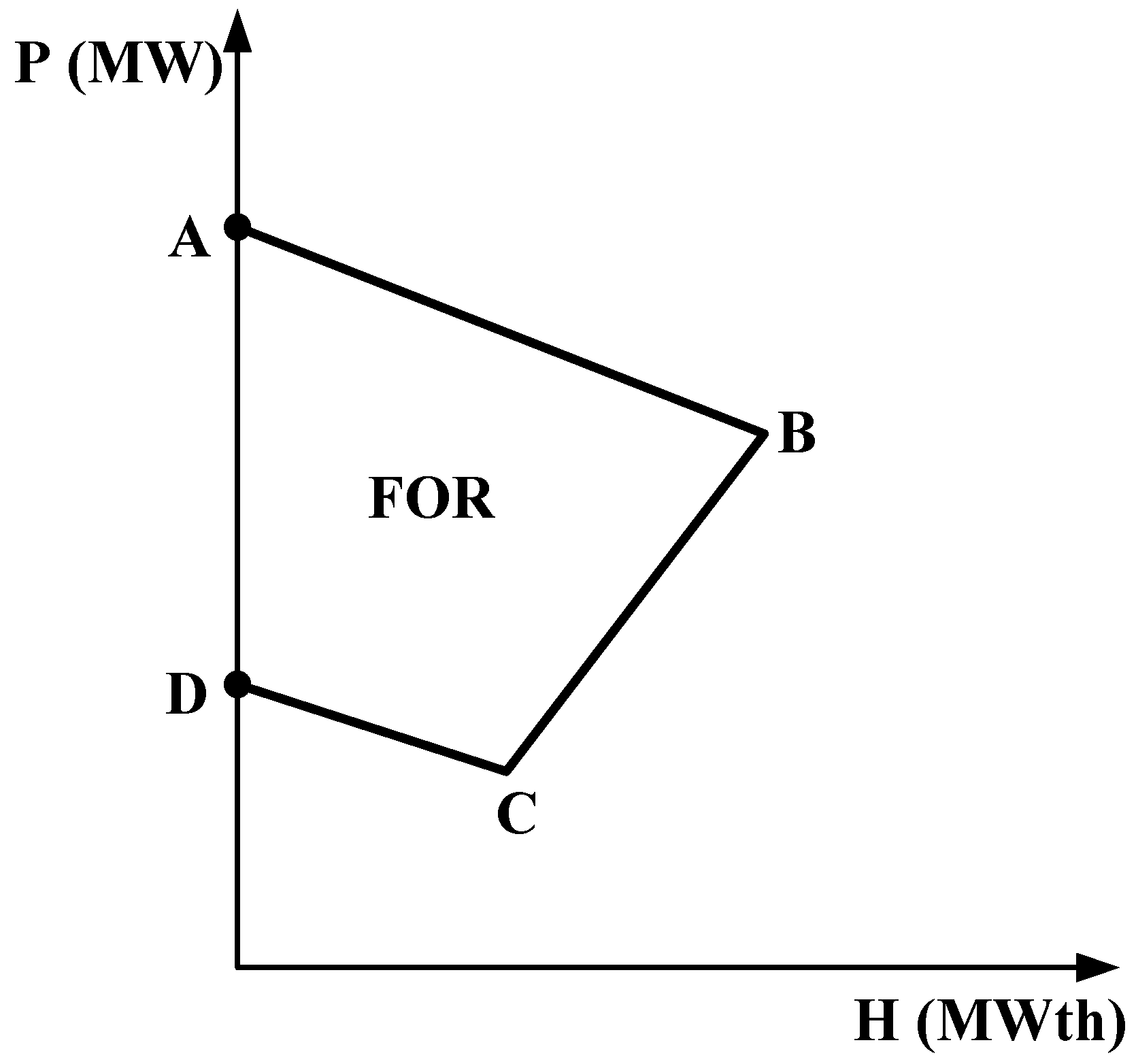
2.6.4. Capacity Limits of CHP Units

The cogeneration unit’s capacity limit is expressed by Equations (15) and (16) [44].

$$P_j^{C, min}\left(h_j^C\right)\le P_j^C\le P_j^{C, max}\left(h_j^C\right);j=1,\dots ,N_C$$

(15)

$$h_j^{C,min}\left(P_j^C\right)\le h_j^C\le h_j^{C,max}\left(P_j^C\right);j=1,\dots ,N_C$$

(16)

In Equations (15) and (16), for the $j^{th}$ cogeneration unit, $P_j^{C,min}\left(h_j^C\right)$ MW and $P_j^{C,max}\left(h_j^C\right)$ MW are the minimum and maximum limits of power generation, respectively, and for the $j^{th}$ CHP unit, $h_j^{C,min}\left(P_j^C\right)$ MWth and $h_j^{C,max}\left(P_j^C\right)$ MWth are the minimum and maximum heat production, respectively.

2.6.5. Capacity Limits of Heat Units

The heat unit’s capacity limit is expressed by Equation (17) [44].

$$h_k^{H,min}\le h_k^H\le h_k^{H,max}:k=1,\dots ,N_H$$

(17)

In Equation (17), for the $k^{th}$ heat unit, $h_k^{H,min}$ MWth is the lowest bound and $h_k^{H,max}$ MWth is the highest bound of heat generation.

2.6.6. Constraint of Prohibited Operating Zones (POZs)

The input–output curve of a device becomes discontinuous due to difficulties in machinery or its parts, such as pumps or boilers, in practical generating units [40,41]. The POZs of a power unit are conveyed by Equation (18).

$$\left\{\begin{array}{c}{P}_i^{T^{min}}\le P_i^T\le P_{i,1}^{T^L}\\ P_{i,m-1}^{T^U}\le P_i^{TH}\le P_{i,m}^{T^L},\hspace{1em}where\hspace{1em}m=\mathrm{2,3},...........Z_i^{}\\ P_{i,zi}^{T^u}\le P_i^T\le P_i^{T^{max}}\end{array}\right.$$

(18)

In Equation (18), $P_{i,m}^{T^L}$ and $P_{i,m}^{T^U}$ are the lowest and highest boundaries of the $m^{th}$ POZ of the $i^{th}$ power unit, and $Z_i^{}$ is the number of POZs.

2.7. Constraint Handling Technique

In this study, the external penalty factor was imposed to handle all constraints. After various trials, the best suitable penalty value was chosen. Assume a function x = (x₁, x₂, …, x_n), which is nonlinear and contains n design variables. The modified objective function is given as follows:

$$\begin{gathered} min c (x_1, x_2,\dots , x_n) \\ {g}_i{(x}_1,x_2,\dots ,x_N)=0;\hspace{1em}where\hspace{1em}i=\mathrm{1,2},\dots ,ne \end{gathered}$$

$$h_j{(x}_1,x_2,\dots ,x_N)\le 0;\hspace{1em}where\hspace{1em}j=\mathrm{1,2},\dots ,nie$$

where $\mathrm{n}\mathrm{e}$ is the equality constraint and $\mathrm{n}\mathrm{i}\mathrm{e}$ is the inequality constraint.

Suppose an infeasible value is $x_1$; then, $g_i$ (${\mathrm{x}}_1$) is not equal to zero for the equality constraint and $h_j$ ($x_1$) is greater than zero for the inequality constraint. For handling this situation, an appropriate value of penalty was imposed. After several trials, a suitable value of R was finalised. The restructured objective function is expressed by Equation (19).

$$f(x)=min c(x_1,x_2, \dots ,x_n) + R({\sum }_{i=1}^{ne}{g}_i^2(x)+{\sum }_{j=1}^{nie}{max(0,h_j\left(x\right)}^2)$$

(19)

3. Rao-3 Optimisation Algorithm

The Rao-3 optimisation technique is an algorithm-specific and parameter-less method to explain constrained and unconstrained optimisation difficulties in a straightforward manner. It has only two control variables, i.e., the size of the population and the maximum number of iterations. The best and worst candidates are selected during the iteration. The Rao-3 algorithm has random interfacing among the candidates [45]. The process flow diagram is given in Figure 3. The algorithm’s steps are outlined below:

Step 1. Model the fitness function: Model an exact fitness function F(X) for the total operating cost of the CHPED. The nature of the function is minimising.

Step 2. Initialise the input variables: Initialise the problem design variables for all generating units. Set the demand in terms of power and heat. Define the size of the search space as n, the control variables as m, and the maximum termination counts.

Step 3. Choose the required outcomes: Find F(X) _best and F(X)_worst, which are the lowest and highest values of the fitness function during the iterative process. Recognise the best and worst values among ${\mathrm{X}}_{\mathrm{j},\mathrm{k},\mathrm{i}}$ of F(X). During the ${\mathrm{i}}^{\mathrm{t}\mathrm{h}}$ iteration, ${\mathrm{X}}_{\mathrm{j},\mathrm{k},\mathrm{i}}$ is the value of the ${\mathrm{j}}^{\mathrm{t}\mathrm{h}}$ control parameter for the ${\mathrm{k}}^{\mathrm{t}\mathrm{h}}$ candidate.

Step 4. Adjust the results: Adjust the result based on the lowest and highest values of F(X) and the random communication among them. in the Rao-3 algorithm based on Equation (20).

$$X_{j,k,i}^{\prime }=X_{j.k.i}+r_{1,j,i}\left(X_{j,best,i}-{|X}_{j,worst,i}|\right)+r_{2,j,i}(|X_{j,k,i} or X_{j,l,i}|-(X_{j,l,i}or{X}_{j,k,i}))$$

(20)

In Equation (20), during the $i^{th}$ iteration, $X_{j,best,i}$ and $X_{j,worst,i}$ are the best and worst values for the variable j. The modified value of $X_{j.k.i}$ is $X_{j,k,i}^{\prime }$ and two random numbers are taken, i.e., $r_{1,j,i}$ and $r_{2,j,i}$ between 0 and 1.

In Equation (20), information is exchanged between the candidates k and l and it is given by the term “$X_{j,k,i} or X_{j,l,i}$”. Finalise $X_{j,k,i},\mathrm{i}\mathrm{f}$ the fitness of candidate k is better than candidate l; otherwise, finalise $X_{j,l,i}$.

Step 5. Finalise the optimum results: Check if the modified value $X_{j,k,i}^{\prime }$ is better than $X_{j.k.i}$; then, take the modified value in place of the previous value corresponding to the fitness function; otherwise, preserve the previous value. Quote the optimum values of the CHPED problem. Repeat the same process until the termination criteria have been satisfied. The methodology is based on the single-objective framework, but in future, it can be extended to multi-objective CHPED formulation.

4. Results and Discussion

This test arrangement comprises 48 units. The number of power units is 26, of cogeneration units is 12, and of heat units is 10. The results are generated with/without the POZs of the power unit. The unit test statistics are taken from ref. [46]. The units of power and heat are represented in MW and MWth, respectively. To demonstrate the economic aspects of wind power generation, a wind energy system with a capacity of 75 MW is used to resolve the CHPED issue. The shape factor is 2, scale factor is 9, and wind speed is 9 m per second. The actual power available, ${\mathrm{P}}_{\mathrm{w}\mathrm{a}\mathrm{v},\mathrm{n}}$, at a given wind speed is 46.4953 MW.The shape factor is 2 and the scale factor is 9 [35,37]. The power demand is 4700 MW and the heat demand is 2500 MWth.

Assume the size of the population is 50 and the maximum iterative count is 1000. Due to the stochastic algorithm’s arbitrary outcomes, the actual measures receive approximately 50 distinct trials. To prove the success of the planned optimisation technique [45], for the CHPED issue, the outcomes were compared with other literature sources. For a more accurate explanation, the test system was classified into two cases, which are explained below.

Case I: Here, only the VPL impact was taken. This test system also considered the renewable energy source to mean a wind turbine. The optimum values of power and heat with or without wind turbine is displayed in

Table 1. Optimal distribution of power–heat production considering VPL effect.

Optimum Points/Algorithm	Rao-3 Optimisation Algorithm
	Without Wind Power Plant	With Wind Power Plant
P1	448.9016	538.5576
P2	150.5174	235.499
P3	299.1002	299.2794
P4	111.9267	159.2979
P5	109.9999	109.3577
P6	61.7496	109.4513
P7	160.9235	110.0024
P8	60.0000	60.3871
P9	159.9627	159.7271
P10	115.0031	40.0000
P11	78.4031	78.4161
P12	90.4963	55.0000
P13	94.9297	55.0010
P14	361.9246	551.3106
P15	223.8261	300.2331
P16	360.0000	299.1706
P17	159.7575	109.7134
P18	60.1047	109.8406
P19	160.0031	109.1617
P20	160.9213	159.9191
P21	164.7013	109.2717
P22	159.7283	109.2472
P23	78.5423	40.0000
P24	40.0000	40.0021
P25	91.1438	55.0000
P26	93.8026	55.0000
P27	93.9081	81.0000
P28	40.0312	40.0000
P29	92.1826	81.0000
P30	50.3218	40.0010
P31	11.001	10.0000
P32	35.0000	35.0000
P33	86.1734	81.1064
P34	41.9321	45.2648
P35	100.0316	81.0000
P36	48.1031	40.0191
P37	10.0000	10.0000
P38	35.0000	35.0000
H27	125.9296	105.8131
H28	76.8746	74.9929
H29	110.4213	105.9921
H30	84.0013	75.0000
H31	40.0000	40.0000
H32	19.9999	19.9999
H33	107.9086	104.9929
H34	80.0301	75.0000
H35	115.9063	104.8899
H36	84.0301	76.9999
H37	39.9999	40.0000
H38	19.0301	20.0000
H39	470.9036	506.1681
H40	60.0000	60.0000
H41	60.0000	60.0000
H42	120.0000	120.0000
H43	119.9998	120.0000
H44	405.1475	430.1987
H45	60.0000	59.9999
H46	59.9926	60.0000
H47	120.0000	119.9999
H48	119.9286	119.9999
Pw	-	62.7620
Pd	4700.0543	4699.998
Hd	2500.1039	2500.0472

. Numerical examinations of the maximum, minimum, and mean costs are displayed in

Table 2. Statistical analysis considering only VPL.

Cost/Algorithm	OGSO [26]	TVAC-PSO [22]	GSA [47]	Rao-3 Optimisation Algorithm
				Without Wind Power Plant	With Wind Power Plant
Minimum cost ($/h)	116,403.3311	117,824.8956	117,266.6810	116,080.6742	115,665.9278
Max cost ($/h)	116,423.9803	-	-	116,807.0083	116,298.9705
Mean cost ($/h)	116,412.6214	-	-	116,459.5012	116,028.7724
Ca ($/h)	-	-	-	116,080.6201	115,665.8650
Cd ($/h)	-	-	-	0.0541	0.0628

. It was found that the minimum cost generated by the proposed algorithm was 116,080.6742 ($/h) and it was less compared to another algorithm, GSA [47]. The insertion of a wind turbine with a CHP unit showed more economically beneficial results. It reduced the cost as well as environmental hazards. The minimum cost obtained was 115,665.9278 ($/h) after considering a wind turbine system. The optimal power sharing, Pw, obtained from the wind turbine is 62.7620 MW. Ca is the minimum calculated cost and Cd is the deviated cost between the calculated cost and the cost attained using the suggested method. It was seen that after the integration of the renewable energy source, the system became more economically beneficial. The minimum cost curve of the planned procedure is revealed in Figure 4.

Case II: Here both VPL impacts and POZ are taken into consideration.

Table 3. Optimal allocation of power and heat generation considering VPL effect and POZs.

Optimum Points/Algorithm	Rao-3 optimisation Algorithm
	Without Wind Power Plant	With Wind Power Plant
P1	179.9998	538.0023
P2	359.6587	224.1854
P3	149.9965	298.6296
P4	60.0000	60.3146
P5	60.0000	109.9267
P6	160.0128	111.1143
P7	159.0098	159.2184
P8	177.2365	156.2358
P9	114.9548	109.1301
P10	111.0125	40.0013
P11	115.2487	40.0000
P12	94.2485	55.0116
P13	55.0000	55.0000
P14	628.9987	628.9006
P15	359.9965	151.8136
P16	299.6507	299.1876
P17	121.8057	174.1376
P18	110.8311	160.8615
P19	60.0000	110.0172
P20	86.0972	109.1392
P21	159.6231	109.8406
P22	60.0000	109.1403
P23	119.9991	114.0926
P24	40.0000	40.0000
P25	108.2158	55.0096
P26	92.8015	55.0000
P27	94.5184	81.734
P28	44.1719	40.0361
P29	94.4329	81.0015
P30	44.0106	40.0013
P31	10.0018	10.0000
P32	45.2846	35.5172
P33	98.2765	81.0340
P34	47.2480	40.0176
P35	87.1258	81.6112
P36	44.2851	40.1372
P37	10.8425	10.0000
P38	35.4597	35.0073
H27	114.9581	104.7216
H28	81.2501	74.0134
H29	104.4857	104.1387
H30	78.5420	75.0000
H31	40.0745	40.0057
H32	24.5480	20.0001
H33	104.2471	104.6872
H34	82.0024	75.1372
H35	109.8548	104.0019
H36	89.9021	75.2476
H37	40.0000	40.0012
H38	20.5049	19.2939
H39	449.1954	506.1939
H40	59.9964	59.5296
H41	60.0000	60.0000
H42	120.0000	119.9296
H43	120.0000	120.0000
H44	440.9541	438.1092
H45	60.0000	59.9929
H46	59.9984	60.0000
H47	119.5486	120.0000
H48	119.9046	120.0000
Pw	-	49.9921
Pd	4700.0558	4700.0001
Hd	2499.967	2500.004

displays the optimum distribution of power/heat production with/without a wind turbine. The numerical measurements of minimum, maximum, and mean cost are displayed in

Table 4. Statistical analysis considering VPL and POZs.

Cost/Algorithm	MPSO [49]	GSO [48]	Rao-3 Optimisation Algorithm
			Without Wind Power Plant	With Wind Power Plant
Minimum cost ($/h)	117,132.4379	117,098.4186	116,986.2277	115,841.3764
Maximum cost ($/h)	-	-	117,868.8103	116,173.7265
Mean cost ($/h)	-	-	117,440.9501	116,035.8226
Ca ($/h)	-	-	116,985.9734	115,841.2456
Cd ($/h)	-	-	0.2543	0.1308

. It was found that the minimum operational price from the proposed method is 116,986.2277 ($/h), which is less compared to GSO [48]. When a wind energy unit is taken with a cogeneration unit, the cost is reduced significantly. The minimum cost calculated with a wind energy system is 115,841.3764 ($/h). The economic impact of considering a renewable energy system is visible, and the optimal power sharing, Pw, obtained from the wind turbine is 49.9921 MW. Ca is the minimum calculated price and Cd is the deviated cost between the calculated cost and the cost attained with the proposed algorithm. The minimum cost convergence curve of the proposed technique is revealed in Figure 5.

5. Conclusions

In the present work, Rao-3 algorithm was applied to resolve the constrained CHPED problem with and without a wind power plant integrated in a typical power system area considering a CHP unit. Most of the metaheuristic algorithm was difficult to handle due to various algorithm-specific parameters. The Rao-3 algorithm can overcome this issue due to less design parameters. To enhance the potential benefits of a basic CHP unit, a wind energy source was inserted. The optimised results of power and heat were calculated considering the VPL effect, the POZs of the power unit, and the FOR of the cogeneration unit. An exterior penalty method was applied to handle the constraints.

The main findings of the article are as follows:

▪

It was observed that after the integration of a wind energy resource, the minimum operating cost decreased significantly.

▪

When considering only the VPL effect, the minimum cost observed from the proposed algorithm was 116,080.6742 (USD/h) and 115,665.9278 (USD/h) in the case of without and with the wind energy plant, respectively.

▪

When considering both the VPL effect and POZs, the minimum cost observed from the proposed algorithm was 116986.2277 (USD/h) and 115841.3764 (USD/h) in the case of without and with the wind energy plant.

▪

The proposed Rao-3 algorithm was found to be suitable to resolve the large-scale CHPED issue, especially with the integration of a wind power plant and considering the operational constraints of the CHP unit.

It was found that the recommended algorithm gave more optimised outcomes for CHPED. The presented work can be further extended by considering the additional limitations of a power unit, such as the ramp rate limit, spinning reserve constraints, etc. Additionally, other renewable energy sources can be added in the power system area for reducing the operational cost and emissions from the thermal power units and finding a solution for managing the intermittency using the dispatchable power capacity of the CHP unit.

References

1. Kazda, K.; Li, X. A Critical Review of the Modeling and Optimization of Combined Heat and Power Dispatch. Processes 2020, 8, 441. [Google Scholar] [CrossRef]
2. Kaur, P.; Chaturvedi, K.T.; Kolhe, M.L. Techno economic power dispatching of combined heat and power plant considering prohibited operating zones and valve point loading. Processes 2022, 10, 817. [Google Scholar] [CrossRef]
3. Wood, J.; Wollenberg, B.F. Power Generation, Operation and Control, 2nd ed.; Wiley: New York, NY, USA, 1996. [Google Scholar]
4. Grainger, J.J.; Stevenson, W.D., Jr. Power System Analysi; McGraw-Hill: New York, NY, USA, 1994. [Google Scholar]
5. Kaur, P.; Chaturvedi, K.T.; Kolhe, M.L. Combined heat and power economic dispatching within energy network using hybrid metaheuristic technique. Energies 2023, 16, 1221. [Google Scholar] [CrossRef]
6. Nazari-Heris, M.; Mohammadi-Ivatloo, B.; Asadi, S.; Geem, Z.W. Large-scale combined heat and power economic dispatch using a novel multi-player harmony search method. Appl. Therm. Eng. 2019, 154, 493–504. [Google Scholar] [CrossRef]
7. Niknam, T.; Azizipanah-Abarghooee, R.; Roosta, A.; Amiri, B. A new multi-objective reserve constrained combined heat and power dynamic economic emission dispatch. Energy 2012, 42, 530–545. [Google Scholar] [CrossRef]
8. Rooijers, F.J.; Van, A. Static economic dispatch for co-generation systems. IEEE Trans. Power Syst. 1994, 3, 1392–1398. [Google Scholar] [CrossRef]
9. Tao, G.; Henwood, M.I.; Van, O.M. An algorithm for heat and power dispatch. IEEE Trans. Power Syst. 1996, 11, 1778–1784. [Google Scholar] [CrossRef]
10. Sashirekha, A.; Pasupuleti, J.; Moin, N.; Tan, C.S. Combined heat and power (CHP) economic dispatch solved using Lagrangian relaxation with surrogate subgradient multiplier updates. Int. J. Electr. Power Energy Syst. 2013, 44, 421–430. [Google Scholar] [CrossRef]
11. Rong, A.; Lahdelma, R. An efficient envelope-based branch and bound algorithm for non-convex combined heat and power production planning. Eur. J. Oper. Res. 2007, 183, 412–431. [Google Scholar] [CrossRef]
12. Su, C.T.; Chiang, C.L. An incorporated algorithm for combined heat and power economic dispatch. Electr. Power Syst. Res. 2004, 69, 187–195. [Google Scholar] [CrossRef]
13. Song, Y.H.; Xuan, Y.Q. Combined heat and power economic dispatch using genetic algorithm-based penalty function method. Electr. Mach. Power Syst. 1998, 26, 363–372. [Google Scholar] [CrossRef]
14. Subbaraj, P.; Rengaraj, R.; Salivahanan, S. Enhancement of combined heat and power economic dispatch using self-adaptive real-coded genetic algorithm. Appl. Energy 2009, 86, 915–921. [Google Scholar] [CrossRef]
15. Huang, S.H.; Lin, P.C. A harmony-genetic based heuristic approach toward economic dispatching combined heat and power. Electr. Power Energy Syst. 2013, 53, 482–487. [Google Scholar] [CrossRef]
16. Geem, Z.W.; Kho, Y.H. Handling non-convex heat-power feasible region in combined heat and power economic dispatch. Electr. Power Energy Syst. 2012, 34, 171–173. [Google Scholar] [CrossRef]
17. Elaiw, A.M.; Xia, X.; Shehata, A.M. Combined heat and power dynamic economic dispatch with emission limitations using hybrid DE-SQP method. Abstr. Appl. Anal. 2013, 2013, 1–10. [Google Scholar] [CrossRef]
18. Bahmani-Firouzi, B.; Farjah, E.; Seifi, A. A new algorithm for combined heat and power dynamic economic dispatch considering valve-point effects. Energy 2013, 2, 320–332. [Google Scholar] [CrossRef]
19. Nwulu, N. Combined heat and power dynamic economic emissions dispatch with valve point effects and incentive-based demand response programs. Computation 2020, 8, 101. [Google Scholar] [CrossRef]
20. Nguyen, T.T.; Vo, D.N.; Dinh, B.H. Cuckoo search algorithm for combined heat and power economic dispatch. Int. J. Electr. Power Energy Syst. 2016, 81, 204–214. [Google Scholar] [CrossRef]
21. Chen, J.; Zhang, Y. A lagrange relaxation-based alternating iterative algorithm for non-convex combined heat and power dispatch problem. Electr. Power Syst. Res. 2019, 177, 105982. [Google Scholar] [CrossRef]
22. Mohammadi-Ivatloo, B.; Moradi-Dalvand, M.; Rabiee, A. Combined heat and power economic dispatch problem solution using particle swarm optimization with time-varying acceleration coefficients. Electr. Power Syst. Res. 2013, 95, 9–18. [Google Scholar] [CrossRef]
23. Roy, P.K.; Paul, C.; Sultana, S. Oppositional teaching learning-based optimization approach for combined heat and power dispatch. Int. J. Electr. Power Energy Syst. 2014, 57, 392–403. [Google Scholar] [CrossRef]
24. Meng, A.; Mei, P.; Yin, H.; Peng, X.; Guo, Z. Crisscross optimization algorithm for solving combined heat and power economic dispatch problem. Energy Convers. Manag. 2015, 105, 1303–1317. [Google Scholar] [CrossRef]
25. Haghrah, A.; Nazari-Heris, M.; Mohammadi-Ivatloo, B. Solving combined heat and power economic dispatch problem using real coded genetic algorithm with improved Mühlenbein mutation. Appl. Therm. Eng. 2016, 99, 465–475. [Google Scholar] [CrossRef]
26. Basu, M. Combined heat and power economic dispatch using opposition-based group search optimization. Int. J. Electr. Power Energy Syst. 2015, 73, 819–829. [Google Scholar] [CrossRef]
27. Pattanaik, J.K.; Basu, M.; Dash, D.P. Heat Transfer Search Algorithm for Combined Heat and Power Economic Dispatch. Iran. J. Sci. Technol. Trans. Electr. Eng. 2019, 44, 963–978. [Google Scholar] [CrossRef]
28. Chen, X.; Li, K.; Xu, B.; Yang, Z. Biogeography-based learning particle swarm optimization for combined heat and power economic dispatch problem. Knowl.-Based Syst. 2020, 20, 106463. [Google Scholar] [CrossRef]
29. Shaabani, Y.A.; Seifi, A.R.; Kouhanjani, M.J. Stochastic multi-objective optimization of combined heat and power economic/emission dispatch. Energy 2017, 141, 1892–1904. [Google Scholar] [CrossRef]
30. Alomoush, M.L. Microgrid combined power-heat economic emission dispatch considering stochastic renewable energy resources, power purchase and emission tax. Energy Convers. Manag. 2019, 200, 112090. [Google Scholar] [CrossRef]
31. Basu, M. Combined heat and power economic emission dispatch using nondominated sorting genetic algorithm-II. Int. J. Electr. Power Energy Syst. 2013, 53, 135–141. [Google Scholar] [CrossRef]
32. Goudarzi, A.; Li, Y.; Xiang, J. A hybrid non-linear time-varying double weighted particle swarm optimization for solving non-convex combined environmental economic dispatch problem. Appl. Soft Comput. 2020, 86, 105894. [Google Scholar] [CrossRef]
33. Hetzer, J. An Economic Dispatch Model Incorporating Wind Power. IEEE Trans. Energy Convers. 2008, 23, 603–611. [Google Scholar] [CrossRef]
34. Liu, X. Optimization of a combined heat and power system with wind turbines. Electr. Power Energy Syst. 2012, 43, 1421–1426. [Google Scholar] [CrossRef]
35. Biswas, P.P.; Suganthan, P.N.; Qu, B.Y.; Amaratunga, G.A.J. Multi objective economic-environmental power dispatch with stochastic wind-solar-small hydro power. Energy 2018, 150, 1039–1057. [Google Scholar] [CrossRef]
36. Hu, F.; Hughes, K.J.; Ingham, D.B.; Ma, L.; Pourkashanian, M. Dynamic economic and emission dispatch model considering wind power under Energy Market Reform: A case study. Electr. Power Energy Syst. 2019, 110, 184–196. [Google Scholar] [CrossRef]
37. Biswas, P.P.; Suganthan, P.N.; Amaratunga, G.A.J. Optimal power flow solutions incorporating stochastic wind and solar power. Energy Convers. Manag. 2017, 148, 1194–1207. [Google Scholar] [CrossRef]
38. Joshi, P.M.; Verma, H.K. An improved TLBO based economic dispatch of power generation through distributed energy resources considering environmental. Sustain. Energy Grids Networks 2019, 18, 100207. [Google Scholar] [CrossRef]
39. Basu, M. Squirrel search algorithm for multi-region combined heat and power economic dispatch incorporating renewable energy sources. Energy 2019, 182, 296–305. [Google Scholar] [CrossRef]
40. Chaturvedi, K.T.; Pandit, M.; Srivastava, L. Self-organising hierarchical particle swarm optimisation for non-convex economic dispatch. IEEE Trans. Power Syst. 2008, 23, 1079–1087. [Google Scholar] [CrossRef]
41. Chaturvedi, K.T.; Pandit, M.; Srivastava, L. Particle swarm optimization with time varying acceleration coefficients for non-convex economic power dispatch. Int. J. Electr. Power Energy Syst. 2009, 31, 249–257. [Google Scholar] [CrossRef]
42. Mellal, M.A.; Williams, E.J. Cuckoo optimization algorithm with penalty function for combined heat and power economic dispatch problem. Energy 2015, 93, 1711–1718. [Google Scholar] [CrossRef]
43. Rabiee, A.; Jamadi, M.; Mohammadi-Ivatloo, B.; Ahmadian, A. Optimal non-convex combined heat and power economic dispatch via improved artificial bee colony algorithm. Processes 2020, 8, 1036. [Google Scholar] [CrossRef]
44. Nazari-Heris, M.; Mohammadi-Ivatloo, B.; Gharehpetian, G.B. A comprehensive review of heuristic optimization algorithms for optimal combined heat and power dispatch from economic and environmental perspectives. Renew. Sustain. Energy Rev. 2017, 81, 2128–2143. [Google Scholar] [CrossRef]
45. Rao, R.V. Rao algorithms: Three metaphor-less simple algorithms for solving optimization problems. Int. J. Ind. Eng. Comput. 2020, 11, 107–130. [Google Scholar] [CrossRef]
46. Zou, D.; Li, S.; Kong, X.; Ouyang, H.; Li, Z. Solving the combined heat and power economic dispatch problems by an improved genetic algorithm and a new constraint handling strategy. Appl. Energy 2019, 237, 646–670. [Google Scholar] [CrossRef]
47. Beigvand, S.D.; Abdi, H.; Scala, M.L. Combined heat and power economic dispatch problem using gravitational search algorithm. Electr. Power Syst. 2016, 133, 160–172. [Google Scholar] [CrossRef]
48. Basu, M. Group search optimization for combined heat and power economic dispatch. Int. J. Electr. Power Energy Syst. 2016, 78, 138–147. [Google Scholar] [CrossRef]
49. Basu, M. Modified particle swarm optimisation for non-smooth non-convex combined heat and power economic dispatch. Electric. Mach Power Syst. 2015, 43, 2146–2155. [Google Scholar] [CrossRef]
Figure 1. Possible operating area of CHP unit.
Processes 11 01232 g001
Figure 2. Block diagram of wind-based CHPED system.
Processes 11 01232 g002
Figure 3. Flow chart of Rao-3 algorithm.
Processes 11 01232 g003
Figure 4. Minimum cost curve considering VPL effect.
Processes 11 01232 g004
Figure 5. Minimum cost curve considering VPL effect and POZs.
Processes 11 01232 g005