Abstract
The traditional circuit breaker fault diagnosis method suffers from insufficient feature information extraction and is easily affected by abnormal signal acquisition. To address this, this paper introduces the phase space reconstruction algorithm to reconstruct the current signal for fault diagnosis based on phase trajectory features. The proposed method uses a first-order forward differencing method and mutual information method to process abnormal data and select the parameters of the reconstruction, then extract overall and local inflection point features to construct a fault feature set. The support vector machine algorithm-based model is trained and tested using actual samples, and the results show that the proposed method can adaptively sample anomalous signals, exhibit strong robustness, and significantly improve the accuracy of fault classification.
1. Introduction
The circuit breaker is a critical device that plays a vital role in controlling and protecting the power system. During its operation, the current timing signal of the breaking coil reflects the operating characteristics of the electromagnetic coil and contains rich information about the operating mechanism, thus characterizing the operating status of the circuit breaker operating mechanism [1,2], extracting the relevant characteristics of the current signal and analyzing and judging it can timely evaluate the operating status of the circuit breaker operating structure and accurately identify the type of fault, providing a technical basis for realizing condition maintenance and improving the stability and reliability of the power system [3,4].
The effectiveness of fault feature extraction for the circuit breaker is critical to the performance of the fault classification model. At present, scholars at home and abroad have conducted a lot of research on the fault feature extraction of high-voltage circuit breaker coil current signals, mainly focusing on signal time-frequency domain analysis. In Reference [5], a time-domain model based on spline interpolation combined with multiscale linear fitting was used to extract features from circuit breaker breaking coil currents, which provided a basis for subsequent circuit breaker fault state analysis. References [6,7] optimized the extraction of multiple feature vectors in the coil current time domain by principal component analysis and relief optimization methods to achieve accurate fault state assessment and improve the diagnosis efficiency. Reference [8] proposed the use of ensemble empirical modal decomposition and wavelet analysis to filter the current signal, combined with the time-domain polarization method for waveform feature extraction, which can effectively improve the feature extraction accuracy and fault diagnosis accuracy.
The time-frequency domain methods mentioned above are based on the linear characteristics of the signal system for analysis. Since the coil current signal generated by the circuit breaker has nonlinear and non-smooth characteristics, only partial and limited information can be obtained from the perspective of this single variable with low accuracy, so the above linear analysis methods have their limitations, and it is difficult to accurately portray the nonlinear characteristics of the coil current signal. Therefore, for the single-variable time series of the circuit breaker coil current signal, another method needs to be introduced that can obtain more information from the high-dimensional space containing dynamic changes.
Currently, the technical method of extracting characteristic parameters in chaotic systems for evaluation and analysis of time-varying nonlinear and nonstationary systems is gaining more and more attention from scholars and is widely used in the field of fault diagnosis. For example, the phase space reconstruction technique is applied for signal characterization. In Reference [9], the phase space reconstruction method is applied for voltage gap detection and feature parameter localization identification, and the accurate detection of gaps can be performed even when the voltage signal is disturbed. Reference [10] transforms the sampling points in the one-dimensional time-series segments to the two-dimensional phase space based on the phase space reconstruction technique and calculates the similarity degree between the time-series segments based on the distribution of discrete points in the obtained two-dimensional phase space, which effectively realizes the real-time diagnosis of the signal fault state. Reference [11] used the phase space reconstruction technique to process the arc current signal, extracted the geometric features and attribute features of the phase plane attractor as the features to discriminate the arc fault, and characterized the change law of randomness and chaos before and after the occurrence of the arc fault. In References [12,13,14], phase space reconstruction was performed on the mechanical vibration signal of a high-voltage circuit breaker. The morphological features, attribute features, and image edge features of phase space trajectory were extracted as feature covariates for fault diagnosis, and good diagnostic results were achieved.
In the phase space reconstruction, the above literature did not consider the phenomenon of abnormal sampling points in the process of monitoring signal acquisition, resulting in the phase space reconstruction may occur at the sampling abnormalities, which cannot correctly describe the original signal structure dynamic state; at the same time, the above literature mainly focuses on the overall characteristics of the phase space trajectory, ignoring the differences in the local characteristics of different fault phase trajectories, which makes it difficult to ensure the diagnosis accuracy of different fault. It is difficult to ensure the accuracy of diagnosis for different fault types.
Therefore, this paper adopts phase space reconstruction technology to study the feature extraction of high-voltage circuit breaker coil current signal, study the influence of signal abnormal data on the phase space reconstruction effect, introduce the abnormal data processing method based on the first-order forward difference algorithm for signal processing, and then determine the reconstruction parameter delay time τ based on the two-dimensional phase space, and carry out phase space reconstruction to obtain the corresponding phase trajectory; secondly, in order to realize the full utilization of phase trajectory, in order to make full use of the phase trajectory information and enhance the differentiation of fault types, the overall features and local features of the phase trajectory are extracted to build a comprehensive fault feature set, which is used to establish a support vector machine fault classification model to achieve accurate diagnosis of different faults in circuit breakers. The experimental results demonstrate that the proposed method for fault diagnosis, which extracts phase trajectory features from signals with abnormal data, achieves an error rate of less than 1.1%. Furthermore, the average error in different fault feature extractions is less than 1.368% even under high noise levels. The accuracy rate for diagnosing different faults using this approach reaches 98.67%, representing a significant improvement over other diagnostic algorithms.
2. Coil Current Temporal Sequence Phase Space Reconstruction and Reconstruction Parameter Determination
In this section, the chaotic characteristics of circuit breaker coil currents are explored, and a novel approach based on phase space reconstruction and adaptive parameter determination is proposed. Specifically, the first-order forward difference method is introduced to determine appropriate adaptive reconstruction parameters for phase space reconstruction, and the resulting trajectories of coil currents in two-dimensional phase space effectively capture the system’s nonlinear dynamic behavior.
2.1. Chaotic Characteristics of Breaker Coil Current Signal
In this paper, the HP550B2 high-voltage circuit breaker is used as the research object, as shown in Figure 1a for its solenoid mechanism to split-close the solenoid structure model. In the process of splitting and closing, the current applied to the coil causes the core of the solenoid to move upward, the spring is released to drive the mechanical parts to move after triggering the closing the button, and any abnormality in the process will affect the change of current in the coil. The equivalent circuit of the solenoid coil is shown in Figure 1b, where US is the circuit power supply, RS is the power supply internal resistance, RL is the coil and wiring equivalent resistance, and the circuit inductance L varies with the position of the closing the button. The coil is energized when the coil circuit receives a break-open command, where the variable inductance L is related to the air gap of the solenoid core. The closing coil current waveform is shown in Figure 1c. From the above analysis, it can be seen that during the closing process of the circuit breaker, the core mechanism, the closing decoupling close, the closing coil body, and other changes, which subsequently cause changes in the coil current time T1, T3, and T5 and the corresponding current I1, I3, and I5, which provides information for identification of faults in the circuit breaker operating mechanism such as core jamming and coil short circuit between turns.
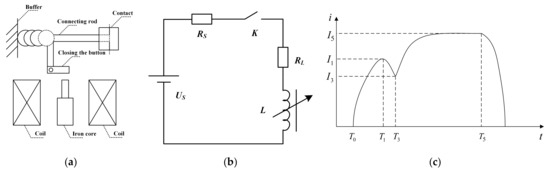
Figure 1.
Model of HP550B2 breaking solenoid with coil equivalent circuit diagram and its closing current waveform: (a) split-close solenoid model; (b) coil solenoid equivalent circuit diagram; (c) coil current waveform.
The phase space reconstruction technique used in this paper is to reconstruct the one-dimensional chaotic time series into the high-dimensional phase space to extract and recover the original laws of the dynamical system. Therefore, prior to the application of this method, it is necessary to ascertain whether the high-voltage circuit breaker coil current signal exhibits chaotic characteristics. Only if this is the case can we analyze the signal using the phase space reconstruction technique.
According to chaos theory, a positive maximum Lyapunov exponent [15] can indicate that the signal has chaotic properties [16]. In this paper, we use the wolf method [17] to calculate the maximum Lyapunov exponent of the normal state during the closing process, where the initial point X(t0) is taken in the reconstruction space, and its distance from the nearest neighbor X0(t0) is set to L0. The time evolution of these two points is tracked until their spacing exceeds a specified value ε > 0 at the moment t1, L′ = |X(t1)−X0(t1)| > ε, Keep X(t1) and find another point X1(t1) adjacent to X(t1) such that L1 = |X(t1)-X1(t1)| < ε and the angle with it is as small as possible. Continue the above process until X(t) reaches the end of the time series, at which time the total number of iterations of the tracking evolution process is M. The maximum Lyapunov exponent is:
where t0 and tM are the initial and end moments; L′i = |X(ti)–X(ti–1)|; Li = |X(ti)–Xi(ti)|.
In order to better analyze the chaotic characteristics of the circuit breaker coil current, take the same operating state of the continuous action test cycle for combined analysis, such as Figure 2a for the normal state of 10 cycles of successive current signals. Among them, Figure 2b shows the Lyapunov exponent spectrum in the normal state, and the maximum Lyapunov calculated by the mean value using the Wolf method is 1.2507 > 0. The calculation results of the current signals in five states are shown in Table 1, and the maximum Lyapunov exponent is greater than 0, indicating that the circuit breaker coil current signal has chaotic characteristics, and the phase space reconstruction technique can be used for subsequent analysis.
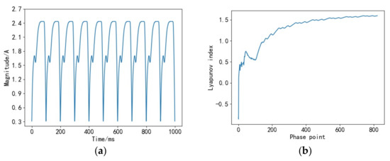
Figure 2.
Normal state multi-cycle current signal with corresponding Lyapunov exponential spectrum: (a) multi-cycle current signal; (b) Lyapunov index spectrum.

Table 1.
Maximum Lyapunov index for different fault states.
2.2. Phase Space Reconstruction of Coil Current Signal
According to Takens’ theorem [18], for a given current time series of length N with , with delay time τ and embedding dimension m, the reconstructed phase space can be expressed as:
where . These K points in the phase space together constitute the current signal time-series phase trajectory.
From Takens’ theorem, it is clear that the choice of τ and m in phase space reconstruction determines whether the reconstructed phase space can accurately reflect the characteristic information of the time series.
Figure 3 and Figure 4 show the variation of the phase trajectory diagram of the coil current time series with different delay time variations when the embedding dimension m = 2, where the variable x(t) is the horizontal axis, and the delay variable x(t + τ) with x(t) is the vertical axis. Figure 3 shows the phase space reconstruction trajectory of the current signal time series in the normal state at the delay time τ = 9. At this time, there is an obvious correspondence between the key points of the time-domain waveform of the coil current signal and the characteristic points of the phase space reconstruction trajectory: the T1 and T3 key points correspond to the trajectory inlet point A, and the T5 key point corresponds to the prominent point B at the top right of the trajectory; as in Figure 4a,b, respectively, the delay time τ = 3 and 15 of the phase space reconstruction trajectories with delay time τ = 3 and 15, respectively. As can be seen from the figure, when the delay time τ is too small, the phase trajectory transformation point A is compressed on the inner trap closed trajectory, and the phase trajectory transformation point B is compressed around the right vertex of the trajectory curve transformation complex; the delay time τ is too large, which will lead to the phase trajectory dispersion and make the component of the phase trajectory feature point A is stretched. Therefore, too large or too small a time delay will result in the current signal in the phase space not being obvious, making the subsequent feature extraction analysis difficult, and a suitable delay time needs to be selected to reconstruct a phase space that can correctly restore the initial signal dynamics information.
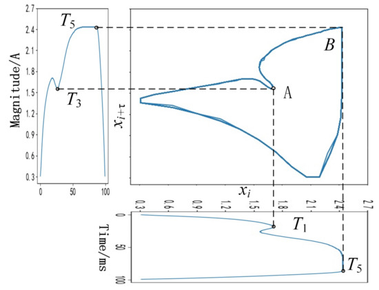
Figure 3.
Phase trajectory at delay time τ = 9 with the characteristics corresponding to the critical point of the current signal.
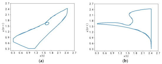
Figure 4.
Phase trajectory with delay time τ = 3, 15: (a) τ = 3; (b) τ = 15.
In addition, since the current signal collected during the actual circuit breaker breaking and closing process has abnormal sampling points in addition to noise, it will likewise have an impact on the selection of reconstruction parameters and subsequent feature extraction.
The acquisition process of the circuit breaker coil current signal is highly susceptible to the actual working conditions, and the acquired signal often appears abnormal. The abnormal data of the signal without considering noise are divided into two categories: one is missing data, and the other is data fluctuation over the limit. The abnormal signal with missing data cannot be reconstructed in phase space and thus cannot obtain the phase trajectory; the current signal with abnormal data fluctuation is shown in Figure 5a. Anomalous fluctuations in data points occurred in the T1–T3 segment of Cycles 3, 4, and 7 and in the vicinity of the T5 characteristic point of Cycles 5 and 6, and the abnormal acquisition in actual working condition basically occurs near the more complex T1–T3 section and T5 time-domain feature points, which is manifested as abnormal fluctuation in itself or the nearby data points, according to which the reconstructed phase trajectory is shown in Figure 5b, corresponding to T1, T3, and T5. The trajectory features of key points are mingled around the phase trajectory corresponding to the abnormal data, which directly affects the extraction accuracy of the subsequent phase trajectory feature points.
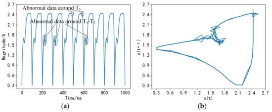
Figure 5.
Current signals containing data fluctuation anomalies and corresponding reconstructed phase trajectory: (a) current signal; (b) reconstructed phase trajectory.
2.3. Adaptive Determination of Phase Space Reconfiguration Parameters
To solve the above problems, this paper proposes an adaptive processing method for the current signal based on the first-order forward differencing algorithm for anomalous data, and then uses the mutual information method to select a suitable delay time τ, so as to realize the adaptive determination of the phase space reconstruction parameters and lay the foundation for the subsequent feature extraction based on the phase trajectory.
2.3.1. Signal Anomaly Data Processing Based on First-Order Forward Differencing
For the lack of current signal data, it is only necessary to check whether the sampling point data are continuous and complete the data; for the signal abnormality in which the signal data fluctuation exceeds the limit described in Section 2.2, the continuous action of the current signal is to collect the abnormal fluctuation exceeding the limit. The differential value of the current signal time series reflects the fluctuation of the signal, and the frequency histogram distribution of the first-order positive differential absolute value of the current signal measuring point containing abnormal fluctuation data is analyzed, as shown in Figure 6.
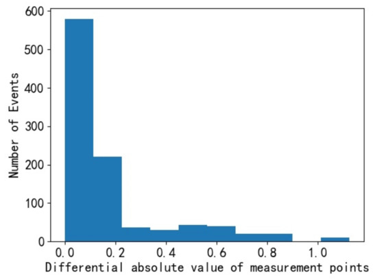
Figure 6.
Frequency histogram distribution of the absolute value of the first-order forward difference.
From the figure, it is found that the frequency of the absolute value of the difference in the interval of 0~0.2 is close to 800, while the frequency of the place where the absolute value of the difference is after 1.0 is low, so the data corresponding to the part of the absolute value of the difference are relatively large and more likely to be abnormal overrun data. Therefore, based on the above analysis, the first-order forward differencing method is introduced for abnormal data processing of the current signal.
For the anomalous data of the current signal, the specific process of filling in the missing data and rejecting the anomalous fluctuation data based on the first-order forward differencing method is as follows.
- (1)
- Firstly, detecting the anomalous missing values of the signal and completing them by linear interpolation.
- (2)
- Secondly, detection of abnormal overrun values based on the first-order forward difference algorithm: the first-order forward difference {xi} is calculated sequentially for the current signal time series Δxi, where Δxi = xi+1 − xi, i = 1, 2, …, N − 1. Then, the threshold λ for judging abnormal overrun data is determined according to the frequency distribution of the absolute value of the difference, and the maximum number of signal abnormal segment data is recorded as n. The number of adjacent consecutive abnormal points in front of xi + 1 is recorded as ei, and k is cycled sequentially from 1 to N − 1. The initial situation ei = 0, i = 0, 1,…, N − 1, and the rules for judging the abnormal overrun data are shown in Figure 7.
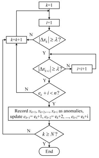 Figure 7. Abnormal overrun data detection.
 - (3)
- Finally, remove the detected abnormal out-of-range points and perform linear interpolation to complete them.
2.3.2. Determination of Delay Time
Since too small a τ will lead to the compression of the reconstructed phase space signal features and too large a τ will lead to the dispersion of the reconstructed phase space signal where no effective features can be obtained, a suitable value of τ must be selected to allow the features to be expressed more effectively. For the circuit breaker coil current signal time series in this paper, the mutual information method [19] is selected to obtain the delay time. The time series of the current signal is x(t), and the time series x(t + τ) via the delay time τ. The mutual information method for selecting the delay time τ is the time corresponding to the first minimal value point of the mutual information function of the general dependence between successive points of the time series as the delay time, where the mutual information function is calculated as:
where Nτ is the length of the time series after the delay, P(i) is the probability that the value of x(t) is i, P(j) is the probability that the value of x(t + τ) is j, and P(i, j) is the joint probability that the value of x(t) is i and the value of x(t + τ) is j.
Take the time series of the circuit breaker coil current with normal signal acquisition as x(t), the time series of the coil current with abnormal acquisition (with abnormal data) as x’(t), and the time series of the coil current after abnormal data processing as x″(t) to calculate the mutual information function of the three, and the correlation change curve between mutual information function and τ is shown in Figure 8.
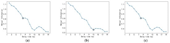
Figure 8.
Mutual information function curve: (a) normal; (b) contains abnormal data; (c) after abnormal data processing.
According to the delay time selection principle of the mutual information method, when the signal is normal without abnormal data, the first local minima of the mutual information function is the point of τ = 8; when the signal has abnormal data, the first local minima of mutual information function is the point of τ = 13; when the signal has abnormal data but after the process of Section 2.3.1, the first local minima of mutual information function is the point of τ = 8. It can be seen that after the signal anomaly data processing based on the first-order forward difference, the first local minima of the current timing mutual information function originally affected by the anomaly data are the same as when the signal is normal without the anomaly data, and the optimal delay time τ is chosen to be the same.
Based on the optimal delay time selected by the above mutual information method and the selected embedding dimension m = 2, the phase trajectories in two-dimensional phase space are shown in Figure 9.
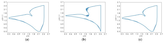
Figure 9.
Phase trajectory comparison chart: (a) normal; (b) contains abnormal data; (c) after abnormal data processing.
The phase trajectories in Figure 9a have an obvious distribution of phase trajectory points A and B in the trapped angle and the right vertex, and the trajectories are uniformly distributed in the phase space as a whole; in Figure 9b, the trajectory trajectories have expanded in the trapped angle, the phase trajectory feature points A are mixed around the phase trajectories corresponding to the anomalous data and the feature components are stretched, and the overall state is diffuse; in Figure 9c, the overall shape of the phase trajectories and the distribution of local trajectory transformation points are basically the same as in Figure 9a.
It can be seen that the presence of anomalous data affects the selection of delay time for phase space reconstruction, resulting in large differences in the overall and local morphology of the reconstructed phase trajectory between the signal with normal acquisition and the signal with anomalous data, which further makes the subsequent phase trajectory analysis and feature extraction difficult, while the introduction of the first-order forward difference-based anomalous data processing method can adapt to the anomalous changes of the signal, and the reconstructed phase trajectory can still maintain stable morphological features when the signal contains anomalous data, thus avoiding the impact of the signal anomalous data on the subsequent signal analysis.
3. Extraction of Feature Parameters for Current Timing Phase Trajectories
The previously proposed phase space reconstruction method is utilized to extract the phase space trajectories of circuit breaker coil currents in different fault states, and their global and local characteristics are obtained. The global features consist of attribute features, such as association dimension D, and morphological features, including origin moments E. Meanwhile, the local features are represented by the amplitudes M1, M3, and M5 of T1, T3, and T5 in the phase space. Analysis of feature distribution reveals that the overall trajectory features cannot fully capture the differences among different fault types. Therefore, combining both global and local features is necessary to achieve a more precise fault diagnosis.
3.1. Phase Space Trajectory of Current Signal
According to the phase space reconstruction method described above, the 10-cycle current time series x(t) of normal and four different faults are taken for phase space reconstruction analysis to obtain the phase trajectory plane diagram. Among them, the single-cycle current signals in different states and the corresponding multi-cycle phase trajectory plots are shown in Figure 10a–f.
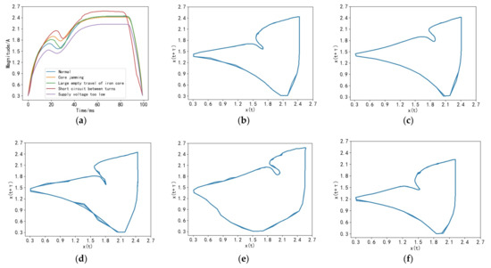
Figure 10.
Current signals in different states and corresponding multi-period phase planes: (a) comparison of time-domain waveforms of current signals under different states; (b) normal state phase trajectory; (c) core card astringent phase track; (d) core empty travel large phase trajectory; (e) inter-turn short-circuit phase trajectory; (f) supply voltage too low phase track.
Combined with Figure 10a–d, the overall difference between current signal waveforms of core jamming and the large core air travel fault state compared with the normal state is small, while the amplitude and time in local T1 and T3 key points have different degrees of rise and delay, which is reflected in the consistency of the overall shape of the corresponding phase trajectory and the offset of local trajectory shift point A in the direction of origin. The diagram of the core empty travel large fault around A point shows that the trajectories are compressed together, making them more susceptible to abnormal data. Combined with Figure 10a,b,e,f, the inter-turn short-circuit supply voltage is too low a fault state compared to the normal state of the overall difference in the current signal waveform, while in the local T1, T3, and T5, the key points have obvious amplitude changes, corresponding to the difference in the overall shape of the corresponding phase trajectory and local key points A and B in the direction of the origin of the obvious offset.
The attractor phase trajectories of the fault current signals in the above figures after phase space reconstruction have different degrees of differences in the overall and local characteristics, and the overall and local characteristics of the phase trajectories can be used to quantitatively characterize their trajectory characteristics and more intuitively and effectively analyze the potential differences before and after the occurrence of the fault.
3.2. Overall Characteristics and Distribution of Attractor Trajectories in Phase Space
- (1)
- Property characteristics of phase trajectories
The correlation dimension reflects the sensitivity to the inhomogeneity of the system attractor and can quantitatively characterize the complexity of the dynamic structure of the attractor [20]. The correlation dimension is used to analyze the attribute of the system attractor, extract the correlation dimension of the attractor trajectory in normal and different fault states, and analyze the change law of the attribute characteristic quantity, so as to better characterize the system chaotic characteristics of the coil current when different states occur. The calculation process of the correlation dimension is as follows:
Calculate the Euclidean distance dij of any two phase points in phase space:
The critical distance variable d is set, and the associated integral Nm(d) is defined as the proportion of all vectors less than d:
where K is the number of state points constituting the phase space trajectory, , .
Determine the association dimension D:
- (2)
- Morphological characteristics of phase trajectories
From the above phase plane diagram, it can be seen that the trajectory of the current signal phase plane attractor as a whole deviates from the origin. In the fault state, the attractor distribution changes, and it is close to or deviates from the origin, so the distance and each state point in the phase plane to the origin is extracted. This is called the origin moment, which can reflect the distribution characteristics of the phase point in the phase space to some extent. The specific expressions are:
where (xi, xi+τ) are the coordinates of the two-dimensional phase plane state points.
Figure 11 shows the distribution of the overall characteristic correlation dimension D and the origin moment E of the phase trajectory for each of the 10 cycles of the current signal in the normal state and the four fault states: the correlation dimension for the normal state fluctuates in the range of 0.48, while the correlation dimension for all four fault states exceeds 0.51, i.e., it is more than 6.25% higher than the normal state, which indicates that the unevenness of the system itself increases after the occurrence of a fault increases, and among them, the correlation dimensions of core jamming, large core air travel, and short circuit between turns, and low supply voltage all fluctuate in the range around 0.52 and 0.56, respectively, which indicates that different fault types will have similar unevenness changes. The normal state origin moment characteristics are distributed in the range of 870~880, while the characteristics of core jamming and large core air travel are all distributed between 880 and 900, with less than 2% change from the normal state and insignificant or even no difference in distribution, but the inter-turn short-circuit and low supply voltage origin moment characteristics are distributed between 910~920 and 790~800, respectively, with a 5% increase and a decrease of about 9%. The analysis of the above results shows that the different types of faults determine the degree of difference of the overall phase trajectory morphology distribution compared with the normal state, and the indicators of core jamming and large core air travel fault states are relatively close to each other, indicating that the phase trajectory morphology of some fault types is similar. Therefore, only the overall phase trajectory characteristics cannot effectively classify and identify each fault state.
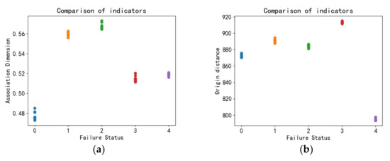
Figure 11.
Overall characteristics of different fault phase trajectories D, E distribution: (a) association dimension D; (b) origin moment E.
3.3. Local Characteristics and Distribution of Attractor Trajectories in Phase Space
Under the premise that the overall characteristics of the phase plane attractor are analyzed in the previous section, further local characteristics of the system attractor are further analyzed in order to improve the variability of the trajectory characteristics of the faulty phase. As the trajectory transition point shown in Figure 3 of Section 2.2, the state coordinates of the two trajectory transition points of the attractor in the normal and fault states are extracted, which are the state coordinates xi and xi + τ of the trajectory transition inlet point A and the state coordinates xi of the trajectory transition protrusion point B, which are noted as the amplitudes M1, M3, and M5 of T1, T3, and T5 in the phase space, respectively.
Figure 12 shows the distribution of the phase trajectory local characteristics M1, M3, and M5 for each of the 10 cycles of the current signal in the normal state and the four fault states; the amplitude M1 under the T1 phase space in the normal state fluctuates in the range of 5.5~5.75, while the M1 of the four fault states has different degrees of change relative to this range, in which the M1 of core jamming, large core empty travel, and inter-turn short circuit, respectively. The T1 value of low supply voltage is reduced by about 11%, while the M1 indexes of core jamming and large core empty travel faults are relatively close to each other; the amplitude of M3 under the T3 phase space in the normal state is distributed between 5.15 and 5.3, and the M3 value distribution of large core empty travel faults has no obvious change relative to the normal state, while other faults have more obvious changes. Meanwhile, the M3 value distribution of core jamming and inter-turn short circuit are 5.8~6.3 and 6.1~6.4, respectively, with overlapping parts; the M5 value distribution under T5 phase space in the normal state is around 8.1~8.15, and the M5 values of core jamming and inter-turn short circuit are in 8.0~8.1 and 8.5~8.6, respectively, with more obvious differences.
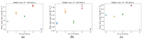
Figure 12.
Distribution of local features M1, M3 and M5 for different fault phase trajectories: (a) amplitude M1 under T1 phase space; (b) amplitude M3 under T3 phase space; (c) amplitude M5 under T5 phase space.
From the above data analysis, it can be concluded that the local features indexes have different degrees of change when different faults occur, which is corresponding to the change of key points of the time-domain model, and the differentiation of fault states can be improved by combining the three local features. Therefore, since the overall features of the trajectory have the defect of incomplete description in the differentiation of fault types, combining these local features with the overall features mentioned above can maximize the differentiation of different fault type features, which can effectively improve the accuracy of subsequent fault identification.
4. Circuit Breaker Fault Diagnosis Process Based on Current Timing Phase Trajectory Feature and Support Vector Machine
The support vector machine [21] (SVM) can use the kernel function to map the feature vectors of the samples to the high-dimensional space and construct the hyperplane in the high-dimensional space to classify the sample feature vectors, which is more suitable for the small sample classification application of coil current signal phase trajectory characteristics. The key to the performance of the SVM model is to select the appropriate penalty parameter C and kernel function parameter g [22,23], to train with the feature parameters of the training samples and the corresponding fault labels, to find the optimal parameters C and g, and then to obtain the optimal classification model.
As shown in Figure 13, the process of circuit breaker fault identification based on current timing phase trajectory characteristics and support vector machine in this paper is as follows:
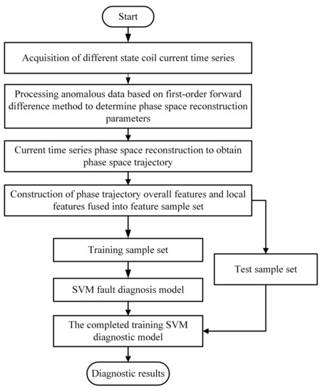
Figure 13.
Overall fault identification process.
- (1)
- Use the anomaly data processing method based on the first-order forward difference algorithm to process the coil current signal with anomaly data, determine the optimal phase space reconstruction parameters on the basis of the processed signal, and carry out phase space reconstruction with these parameters.
- (2)
- Obtain the phase space trajectories of the coil current signals under different fault states, extract the overall features and local features of each phase trajectory, and constitute the sample set of phase trajectory fault features [D,E,M1,M3,M5].
- (3)
- The fault feature sample set is configured as the training set and the test set, the training set is input to the support vector machine model for training, and the model parameters are optimized to establish the fault diagnosis model based on phase trajectory fault feature-SVM. Finally, the test set is used to test the adaptive fault diagnosis performance of this model.
5. Test Results and Analysis
In this paper, the HP550B2 high-voltage circuit breaker is used for testing experiments, simulating five states of normal closing, core jamming, large core air travel, and low power supply voltage for inter-turn short circuit in the closing process; 40 groups of each of the above five state current signals are collected using current sensors, 25 groups are taken as training samples, and the remaining 15 groups are used as test samples. Firstly, the adaptiveness and robustness of the diagnostic model in fault feature extraction are verified and analyzed by introducing abnormal data and noise, and then the diagnostic performance of the model based on different algorithms and different feature indicators are compared.
5.1. Adaptation Analysis of Phase Trajectory Feature Extraction
To analyze the adaptability of feature extraction in the case of acquisition signal with abnormal data, the signal without abnormal data in the acquisition process is noted as I, the signal with abnormal data introduced is Ierror, and the average error is:
where XiI is the i-th fault feature indicator of the signal without abnormal data, XiIerror is the i-th fault feature indicator of the signal with abnormal data, n is the number of phase trajectory feature indicators, and the same feature indicators of different fault states have been normalized. Table 2 describes some of the results of extracting phase trajectory feature indicators for signals with and without abnormal data in each fault state of the circuit breaker. Based on the table of results, it is apparent that the average error range for extracting all state trajectory features falls between 0.702% and 1.064%. Furthermore, even for the core air travel large fault feature extraction, which is highly susceptible to abnormal data, the average error rate is just 1.064%. These findings demonstrate that the proposed method of phase space reconstruction based on the first-order forward difference algorithm can effectively extract phase trajectory features from signals containing abnormal data, with an error rate of less than 1.1%, and the feature indicator values of signals containing abnormal data are obtained more accurately, indicating that the method can be adaptive to the extraction of signal features containing abnormal data. It shows that the method is adaptive to the extraction of signal features of anomalous data.
Table 2.
Selected results of extracted phase trajectory characteristic indexes.
5.2. Robustness Analysis of Phase Trajectory Feature Extraction under Noise
However, the signals collected in real operating situations are usually accompanied by noise in addition to the anomalous data mentioned in this paper, which affects the performance of the diagnostic model. For example, Figure 14 shows different state current waveforms with 40 dB noise, and the algorithm model needs more stable feature extraction capability in the case that the current waveforms contain different levels of noise. Therefore, to test the robustness of the algorithm model proposed in this paper, different proportions of noise are added to the initial coil current signal with signal-to-noise ratios of 40 dB, 35 dB, 30 dB, 25 dB, and 20 dB, respectively, and further tested at the phase trajectory feature extraction based on different fault state current signals, and the test results are shown in Table 3, where the average error is calculated as described in Section 5.1 (where XiIerror is the noise containing signal).
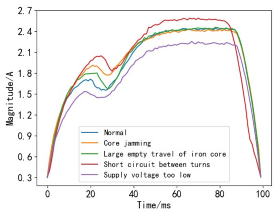
Figure 14.
Current waveform with noise.
Table 3.
Average error of phase trajectory feature extraction under different levels of noise.
From the data in the table, it can be seen that the average error of phase trajectory feature extraction increases with the increase in noise severity (i.e., the signal-to-noise ratio decreases) for the current signals of different fault states, but the range of change is small, and even in the case of only a 20 dB signal-to-noise ratio, the highest average error in each state is 1.101% to 1.368%, which shows the good robustness of phase trajectory feature extraction of the method in this paper under different degrees of noise environment.
5.3. Comparison of Different Algorithmic Models
The fault feature set [D,E,M1,M3,M5] is constructed after the phase trajectory fault features of the circuit breaker current signal are extracted; the training set is input to the SVM model for training; the cross-validation method is used to obtain the model parameters C = 3.24 and g = 1.52, respectively; and the test set is input to the constructed SVM model for fault diagnosis test, and the accuracy of fault diagnosis is 98.67%.
In order to further verify the superiority of the algorithm model of this paper, the algorithm of this paper is compared with other commonly used machine learning classification algorithms, and the input features are compared with the time-domain current signal features and the phase trajectory features proposed in this paper for fault identification accuracy comparison. The algorithm aspect compares the performance of k-nearest neighbor [24] (KNN) and back propagation neural network [25] (BPNN, using the network seeking method to determine neurons and genetic algorithm to determine weights and bias parameters [26]) to identify faults under the same training samples and test samples, respectively. When the time-domain current signal features are set to the feature set [T1,T3,T5,I1,I3,I5] constructed from the time-domain features in Section 2.1, the training and test sample configurations are the same as the phase trajectory feature samples. The test comparison results are shown in Table 4.
Table 4.
Accuracy of different classification models and input features.
From the analysis of the results in the above table, when phase trajectory features are used as input instead of time-domain current signal features, the diagnostic accuracy of the three classifiers is improved by 5.33%, 5.33%, and 4%, respectively. Therefore, using phase trajectory features as input can improve the accuracy of identifying circuit breaker faults. The accuracy rates of the three classifiers are 78.66%, 93.33%, and 98.67% when using phase trajectory features as input, with SVM having significantly higher accuracy rates than other algorithms.
6. Conclusions
This paper studies the distribution trajectory of the circuit breaker opening and closing coil current signal in the phase space, and establishes a circuit breaker fault diagnosis model based on coil current phase trajectory characteristics-SVM. Five different fault states of high-voltage circuit breakers were simulated for diagnostic testing, and the following conclusions were drawn:
- (1)
- The preprocessing method employed, based on the first-order forward difference method, can adaptively eliminate anomalous data, resulting in an accurate reconstruction of phase trajectory characteristics of the coil current signal.
- (2)
- Incorporating local phase trajectory characteristics enables maximum differentiation of different fault states, effectively solving the challenge of classifying similar phase trajectory patterns between certain faults, such as core jamming and large core air travel.
- (3)
- Experimental verification confirms that the proposed fault diagnosis model has strong robustness in feature extraction against interference, with an average error of approximately 1% when the signal-to-noise ratio of noise is between 20 and 40 dB. Furthermore, utilizing phase trajectory features and SVM algorithm models results in significantly improved fault identification accuracy compared to the traditional diagnosis model based on time-frequency domain feature classification algorithms.
However, due to the large number of models of circuit breakers and their operating mechanisms and various types of faults, this study was conducted under common faults that can be simulated. For some faults that are difficult to simulate and cause irreversible damage to the circuit breakers, this method needs to be further validated due to the lack of sample data.
Author Contributions
Conceptualization, Y.C. and Q.L.; Data curation, Y.C.; Investigation, G.L.; Methodology, Y.C. and Q.L.; Project administration, R.F.; Resources, Q.L.; Software, Q.L.; Supervision, Y.Z.; Validation, Y.C.; Visualization, N.Y.; Writing—original draft, Y.C.; Writing—review and editing, Q.L. All authors have read and agreed to the published version of the manuscript.
Funding
This research was funded by State Grid Jiangxi Electric Power Co. Project, grant number 52182023000L and The APC was funded by National Natural Science Foundation of China, grant number 52267008.
Institutional Review Board Statement
Not applicable.
Informed Consent Statement
Not applicable.
Data Availability Statement
Not applicable.
Conflicts of Interest
The authors declare no conflict of interest.
References
- Lu, H.; Ilihamu, Y.; Liu, P.; Zhang, P.; Li, Z.; Kari, T. High Voltage Circuit Breaker Fault Diagnosis Based on GWO-SVM. Comb. Mach. Tools Autom. Mach. Technol. 2022, 103–107. [Google Scholar] [CrossRef]
- Peng, Z.; Wang, S.; Yi, L.; Liu, Q.; Chen, X.; Liang, M.; Chu, F.; Cao, C.; Yan, H.; Liu, D. Research on fault diagnosis of high voltage circuit breaker breaking and closing coil based on SVM principal component analysis. High Volt. Appl. 2019, 55, 39–46. [Google Scholar] [CrossRef]
- Pang, X.; Gan, Y.; Long, Y.; Xiu, S. Research on the diagnosis technology of SF6 circuit breaker interrupter defect based on gas decomposition products. J. Electr. Mach. Control 2020, 24, 122–130. [Google Scholar] [CrossRef]
- Hu, J.; Zhang, W.; Cao, D.; Wen, Y.; Rong, Y. Research on the health condition of power system based on fuzzy theory. Power Syst. Prot. Control 2016, 44, 61–66. [Google Scholar]
- Yang, W.; Ke, Y.; Zhu, S.; Li, B.; Chen, Z.; Zhao, C.; Song, D.; Yang, H. High voltage circuit breaker spring mechanism condition detection based on spline interpolation and linear fit analysis. High Volt. Appl. 2017, 53, 147–153. [Google Scholar] [CrossRef]
- Fan, H.; Li, X.; Su, H.; Chen, L.; Shi, Z. Research on circuit breaker fault diagnosis method based on principal component analysis-support vector machine optimization model. High Volt. Appl. 2020, 56, 143–151. [Google Scholar] [CrossRef]
- Zhang, H.; Zhao, L.; Jing, W.; Yang, W.; Jiang, H.; Zhu, L.; Rong, Q.; Fu, R. Condition evaluation of circuit breaker operating mechanism based on Relief eigenvolume optimization and SOM network. High Volt. Appl. 2017, 53, 240–246. [Google Scholar] [CrossRef]
- Sun, Y.; Zhang, W.; Zhang, Y.; Li, S.; Liu, X. Extraction of high voltage circuit breaker breaking coil current signal features and fault discrimination method. High Volt. Appl. 2015, 51, 134–139. [Google Scholar] [CrossRef]
- Wang, N.; Ma, Z.; Jia, Q.; Dong, H. Voltage gap detection and feature parameter identification based on phase space reconstruction. Chin. J. Electr. Eng. 2017, 37, 5220–5227. [Google Scholar] [CrossRef]
- Wu, X.; Dong, Y.; Hou, Z.; Cheng, W. Extraction of event-based time series segments based on phase space reconstruction. Vib. Shock. 2020, 39, 39–47. [Google Scholar] [CrossRef]
- Cui, R.; Li, Z.; Tong, D. Aero-arc fault detection based on phase space reconstruction and PCA. Chin. J. Electr. Eng. 2021, 41, 5054–5065. [Google Scholar] [CrossRef]
- Li, Z.; Wei, L.; Han, D.; Teng, W. Research on mechanical fault diagnosis of high-voltage circuit breaker based on phase space reconstruction. Power Syst. Prot. Control 2018, 46, 129–135. [Google Scholar]
- Xia, X.; Lu, Y.; Su, Y.; Yang, J. Mechanical fault diagnosis of high-voltage circuit breaker based on phase space reconstruction and improved GSA-SVM. Electr. Power 2021, 54, 169–176. [Google Scholar]
- Sheng, J.; Yin, X.; Deng, W.; Yuan, H.; Yang, A.; Wang, X.; Rong, M. Extraction of edge features of circuit breaker vibration signal based on phase space reconstruction technique. High Volt. Appl. 2022, 58, 27–36. [Google Scholar] [CrossRef]
- Lorenz, E.N. Deterministic Nonperiodic Flow. J. Atmos. Sci. 1963, 20, 130–141. [Google Scholar] [CrossRef]
- Ruan, J.; Yang, Q.; Huang, D.; Zhuang, Z. Chaotic attractor morphology characteristics of mechanical vibration signal of high voltage circuit breaker. Power Autom. Equip. 2020, 40, 187–193. [Google Scholar] [CrossRef]
- Wolf, A.; Swift, J.B.; Swinney, H.L.; Vastano, J.A. Determining Lyapunov Exponents from a Time Series. Phys. D Nonlinear Phenom. 1985, 16, 285–317. [Google Scholar] [CrossRef]
- Takens, F. Detecting Strange Attractors in Turbulence. In Dynamical Systems and Turbulence, Warwick 1980; Rand, D., Young, L.-S., Eds.; Lecture Notes in Mathematics; Springer: Berlin/Heidelberg, Germany, 1981; Volume 898, pp. 366–381. ISBN 978-3-540-11171-9. [Google Scholar]
- Albers, D.J.; Hripcsak, G. Estimation of Time-Delayed Mutual Information and Bias for Irregularly and Sparsely Sampled Time-Series. Chaos Solitons Fractals 2012, 45, 853–860. [Google Scholar] [CrossRef]
- Liu, Y.; He, H.; Xiao, J. Characterization of the correlation dimension of the dynamic pressure at the outlet of a centrifugal compressor. J. Aerodyn. 2021, 36, 300–309. [Google Scholar] [CrossRef]
- Cortes, C.; Vapnik, V. Support-Vector Networks. Mach. Learn. 1995, 20, 273–297. [Google Scholar] [CrossRef]
- Jannah, N.; Hadjiloucas, S. A Comparison between ECG Beat Classifiers Using Multiclass SVM and SIMCA with Time Domain PCA Feature Reduction. In Proceedings of the 2017 UKSim-AMSS 19th International Conference on Computer Modelling & Simulation (UKSim), Cambridge, UK, 5–7 April 2017; IEEE: Piscataway, NJ, USA; pp. 126–131. [Google Scholar]
- Li, Y.; Zhang, R.; Guo, Y.; Huan, P.; Zhang, M. Nonlinear Soft Fault Diagnosis of Analog Circuits Based on RCCA-SVM. IEEE Access 2020, 8, 60951–60963. [Google Scholar] [CrossRef]
- Li, B.; Qi, W.; Yang, Z.; Chen, C.; Gui, Y.; Ren, Z.; Yao, Y.; Wang, H.; Tu, S. High voltage circuit breaker fault diagnosis based on multi-feature selection method. High Volt. Appl. 2020, 56, 218–224. [Google Scholar] [CrossRef]
- Rumelhart, D.E.; Hinton, G.E.; Williams, R.J. Learning Representations by Back-Propagating Errors. Nature 1986, 323, 533–536. [Google Scholar] [CrossRef]
- Yan, R.; Lin, C.; Song, W.; Gao, S.; Zhong, L.; Zhang, W. High Voltage Circuit Breaker Fault Diagnosis Based on EEMD and Convolutional Neural Network. High Volt. Appl. 2022, 58, 213–220. [Google Scholar] [CrossRef]


Disclaimer/Publisher’s Note: The statements, opinions and data contained in all publications are solely those of the individual author(s) and contributor(s) and not of MDPI and/or the editor(s). MDPI and/or the editor(s) disclaim responsibility for any injury to people or property resulting from any ideas, methods, instructions or products referred to in the content. |
© 2023 by the authors. Licensee MDPI, Basel, Switzerland. This article is an open access article distributed under the terms and conditions of the Creative Commons Attribution (CC BY) license (https://creativecommons.org/licenses/by/4.0/).