Article

Shewhart Control Charts Implementation for Quality and Production Management

by
Marcela Malindzakova
1,
Katarína Čulková
2,* and
Jarmila Trpčevská
2
1
Faculty BERG, Technical University of Košice, 042 00 Košice, Slovakia
2
Faculty MMR, Technical University of Košice, 042 00 Košice, Slovakia
*
Author to whom correspondence should be addressed.
Processes 2023, 11(4), 1246; https://doi.org/10.3390/pr11041246
Submission received: 22 February 2023 / Revised: 4 April 2023 / Accepted: 13 April 2023 / Published: 18 April 2023
(This article belongs to the Special Issue 10th Anniversary of Processes: Women's Special Issue Series)

Abstract

:
Shewhart control charts are suitable for stable but repetitive production processes used for the subsequent identification of random deviations while indicating breached quality limits. They provide information on process variability and, at the same time, make it possible to obtain information on the reliability of monitored processes. The objective of this paper is to assess the quality characteristics of plastic mouldings for the needs of the automotive industry with the application of the control charts method, specifically Shewhart control charts. The Shewhart control charts were applied to evaluate the quality characteristics, or, more specifically, to evaluate the measured width and length of the produced plastic mouldings by statistical analysis. Statistical analyses show that the set parameters are not met in the first two days of the test series. An improvement in the process is observed on the last day of the test series. The process is well set, as confirmed by our verification of the stability of the process. An important condition for setting the control charts is to observe the correct chronological arrangement and regular acquisition of measured values. Solving tasks in the future must be oriented to an evaluation of the capability of the production process of the monitored product. The proposal for future research will be oriented toward the evaluation of this capability via process capability indices that derive continuous data by using the classical method.

1. Introduction

The production and processing of plastic moulding constitutes an important industry, as many traditional materials are replaced by cheap and inexpensive plastic materials. Plastics are characterized by high specific strength, comparable thermal stability with excellent chemical resistance, low cost, and their extremely light weight. Plastic materials are an integral part of the modern lifestyle, and their use has increased significantly over the past three decades. The total production of plastic materials in 2021 was 350.7 million tons. European plastics production reached 57.2 Mt. PP, PVC, and HDPE are the major contributors to the total production of plastics in the world. Due to its versatile application and advantages, the consumption of plastic materials is increasing day by day. In 2021, packaging, and building and construction applications were the two largest global plastics markets (www.plasticseurope.org, accessed on 2 January 2023) [1].
This material also has highly beneficial properties in terms of shaping possibilities. By using suitable procedures, it is possible to achieve a huge variability of shapes. In order to maintain consistent quality level, it is possible to apply the Shewhart control chart to ensure the smooth running of the moulding production process.
By definition, statistical process control (SPC) is a highly powerful tool used to reduce the amount of variability to stabilise the process. Statistical process control problem solving can be implemented in any process. Additionally, SPC data can be used to predict future process performance. If the process is stable but operates outside of the required specification limits, the causes for the failures can be identified, removed, and the process thus improved [2,3,4,5,6,7]. Processes will often operate in the in-control state for relatively long periods. However, even if the process is relatively stable for a certain period of time, no process can remain stable forever. Due to some determinable causes, every process will eventually move to an unbalanced state with output parameters outside of the limit requirements. The role of an SPC tool is to specifically identify such causes before their full effect occurs. Subsequent process analysis and corrective measures can prevent non-conforming process outputs from being produced [7].
From this toolset, the control chart is the most sophisticated approach. The control charts are named after Walter A. Shewhart and are a popular tool implemented within industrial processes, particularly when more than one variable needs to be controlled [3]. A great advantage of the control chart is it allows for the identification of change points in time series and excess variability of a process. This functionality, along with its applicability in real-time conditions, makes this SPC method highly suitable as an early failure warning prevention system [5].
The popularity of control charts is primarily attributed to their functionality, as they provide a reliable approach to the increase of productivity and offer diagnostic data in order to evaluate the capability of a process. This can be achieved by implementing pc technology that monitors and analyses these data in real time. Therefore, the careful implementation of control charts can improve the performance of a process by identifying possible failures [3]. They present a graphical method by which a comparison is made based on the number of samples that represent the investigated system. This is done in order to establish limits that consider the typical process variability [4].
In practice, two main types of control charts are used, namely variables control charts and attributes control charts. Each one includes two categories, based on whether the standard value is specified or not. The selection of the relevant category should be based on the quality attributes, on the specification of controlled parameters, and on the quality requirements of the given product. Other specifications for the creation of control charts include the sample size of the data provided, the number of sampling units, the specification of control limits, and the central line. Once control charts are constructed, it can be determined whether the process is stable or not [8].
The research observed so far does not take into account the implementation of Shewhart’s control diagrams for the needs of the production of plastic mouldings. The optimal setting of monitored parameters contributes to the realization of the continuous operation of the production process and to ensuring customer satisfaction. This paper proposes a methodological framework for improving the quality parameters of plastic mouldings. The goal of this paper is to determine the possible implementation of the Shewhart control chart in the practical conditions of an industrial company that had not statistically managed the quality of their output, with an aim to establish possible deformations of the products during the production process. From a strategic point of view, the vision of the company is focused not only on its development, but above all on ensuring its success in the market. The scientific contribution of the presented contribution lies in the constant improvement, innovation and advancement of the company to a higher level both in terms of technology and in terms of quality in order to ensure the requirements of customers in the market are met. In connection with the specific requirements of customers for products, the number of products that are “tailor-made” for each customer is growing significantly. The investigated company is focused on the production of specific products and for this reason it is necessary to control the stability of the production process.

2. Literature Review

Efficient online quality control monitoring using control charts is a strategic aspect of eliminating or reworking scrap to meet demand at the time specified by the production plan. Starting the online monitoring of a quality characteristic by means of a control chart at the beginning of a short production run is often a challenging issue for quality practitioners. In the study of Castagliola et al. (2013), adapted control charts that had typically been implemented with success in long runs to increase the performance of the variable sample size strategy, were investigated for a chart used in a short run [9]. The statistical performance of the VSS t-chart was compared with that of the fixed-parameter (FP) t-chart for scenarios representing both fixed and unknown shift size, with the latter a frequent situation in short-run manufacturing environments.
In the following year several authors studied the area of control charts, such as Celano et al. (2012), who examined the way in which SPC inspection cost optimization is constrained by the configuration of the manufacturing and the inspection activities [10]. Their study aimed to evaluating the economic performance of the Shewhart t-chart versus the Shewhart chart with known parameters. The expected economic loss associated with the implementation of the Shewhart t-chart is acceptable with respect to the ideal condition—a control chart with known parameters and where the cost optimization is achieved without a statistical constraint limiting the number of expected false alarms. Additionally, Li and Pu (2012) made an evaluation and computation based on statistical performance measures for the two-sided Shewhart, cumulative sum, and exponentially weighted moving average control charts for short-run production [11]. Their study compares the efficiency of the three charts and the corresponding Q charts in the cases of known and unknown nominal values of process parameters. Tasias and Nenes (2012) presented a new statistical process control model for the economic optimization of a variable-parameter control chart monitoring a process operation where two assignable causes may occur, one affecting the mean and the other the variance of the process [12]. Their study used an economic (or an economic/statistical) optimization criterion for the time to the next sampling instance, the size of the next sample, as well as the control limits of the inspection. That is, all design parameters of the control scheme were selected so as to minimize the total expected quality-related costs.
Bersimis et al. (2007), searched the basic procedures for the implementation of multivariate statistical process control via control charting, while also reviewing multivariate extensions for all kinds of univariate control charts, such as multivariate Shewhart-type control charts, etc. [13]. In addition, the study reviewed unique procedures for the construction of multivariate control charts, based on multivariate statistical techniques and partial least squares.
Consequently, Zhou and Tsung (2011) developed a new multivariate SPC methodology for monitoring location parameters [14] in order to formulate the charting statistic by incorporating the exponentially weighted moving average control (EWMA) scheme. This control chart possesses some other favourable features: it is fast to compute with a similar computational effort to the MEWMA chart; it is easy to implement; and it is also very efficient in detecting process shifts.
Nenes et al. (2014) investigated a Shewhart control chart in a process with finite production horizon because, when the production horizon is finite, the statistical properties of a control chart are known to be a function of the number of scheduled inspections [15]. The study orientates to a short run producing a finite batch. In 2014, Chowdhury et al. (2014) also studied a distribution-free Shewhart-type chart according to the Cucconi statistic, called the Shewhart–Cucconi (SC) chart [16]. Additionally, they proprosed a follow-up diagnostic procedure useful to determine the type of shift that the process may have undergone when the chart signals an out-of-control process. Li (2015) proposed a new nonparametric multivariate phase-II control chart, not dependent on any tuning parameter and considered to be a natural generalisation of the generalised likelihood ratio chart to the nonparametric setting [17]. The study showed that the proposed control chart performs well across a broad range of settings and compares favourably with existing nonparametric multivariate control charts.
Qiu (2018) gives some perspectives as to the robustness of conventional SPC charts and the strengths and limitations of various nonparametric SPC charts [18]. Mukherjee and Marozzi (2021) found that most of the charts are not robust when the real process parameters are unknown [19]. During their study, they proposed Shewhart-type nonparametric monitoring schemes based on specific distance metrics for the surveillance of multivariate and high-dimensional processes.
The literature does not provide sufficient studies of the use of control charts in areas of plastic moulding. Therefore, the goal of this contribution is to use control diagrams to ensure the operation of the production process and to provide important information about the process. The direct use of Shewhart control charts will then contribute to the optimization of economic aspects, as well as to increase the accuracy of the dimensions of the moulding products. In the case of this research, there is a particular emphasis on the width and length of the moulding.
The aim of the paper is to suggest the use of a Shewhart control chart for the statistical management of production quality. The topic is important because the literature does not provide research in the area of moulding. This method seems to be the most proper for such conditions.

3. Materials and Methods

3.1. Plastic Injection

A variety of technologies are used to process plastics, depending on the technological properties of the plastic used, as well as the shape and function of the final product. At present, injection moulding is the most widely used method. It is a cyclic discontinuous process. The injection moulding process is suitable for all types of plastics. The principle of injection moulding is that the prepared molten material is injected into the cavity of the metal mould, which, after solidification, forms a finished product. This technology can produce complex products with good dimensional tolerances and a good surface finish. The disadvantage of this technology is the high initial cost of the technology and of the moulds (Figure 1).
The actual injection process has well-defined steps. The initial phase is the removal of the granules from the hopper—a helix is placed into the melting chamber by the action of pressure and by the supplied heat by which the granules are plasticized, i.e., by which they become liquid. In the next phase, the plastic is input into the cavity of the mould by moving the helix as a piston, where it cools. However, during cooling the volume decreases, which could cause dents and nicks. Through subsequent overpressure, achieved by pressing another material during cooling, the formation of depressions and sink marks is prevented. This pressure can be the maximum pressure, or weaker. After the product part has partially cooled, the mould is opened, and the finished part is removed from the mould (Figure 1). The whole cycle repeats [20,21,22,23].
The data come from the verification series. The specified quality features are measured for all products, namely the width and length of the product. A digital calliper measures the dimensions (Figure 1).
The quality benchmarks dictate the variability tolerance for the dimensions of the product, specifically its length and width. The data were obtained during a verification series, in which the widths and lengths of all 30 produced pieces were measured within three production days.
Shewhart control charts were used to evaluate the results. Shewhart control charts were used, since they assess the ability of the process to meet the criteria set by the customer, namely compliance with the specified limits and variability around the desired value. Shewhart control charts are useful for identifying deviations that indicate non-compliance with quality limits. The proposed methodological framework is subsequently implemented in a real case study of a company focused on the field of automobile production. The research aims at improvement, innovation, and advancement to a higher level, not only in terms of technology but also in compliance with quality parameters in order to satisfy the demands of customers on the market. During the research we processed according to the process, illustrated in Figure 2.
For the correct application of Shewhart control charts it is necessary to verify three assumptions normalities of data: constant mean, constant standard deviation, and data independence. The normality of the data is tested by the Pearson test of normality and the Kolmogorov test as well as by a rapid test for determining normality, namely the test of normality for asymmetry or excess. The paper applies Pearson’s normality test to test the data normality.

3.2. Specification of Control Diagrams

To verify the stability of the process, it is appropriate to apply Shewhart’s control charts. Shewhart has introduced control charts that serve the needs of statistical process control. The actual control diagram (see Figure 3) shows the monitored parameters in a traditional xy-chart, where the x-axis represents the time sequence and the y-axis the measured values for the monitored parameter (width and length of the product). The chart is continuously updated at regular intervals and thus provides a continuous overview of the current situation of the process. These control charts measure and compare the control. A combination of a control diagram for the arithmetic mean and a control diagram for the variation range evaluates the parameters of the product (moulding).

3.3. Control Diagram for the Range of Variation and Control Diagram for the Arithmetic

Control diagram for the selection range of variation [24,25]
Test   criterion   R j = x m a x . , j x m i n . , j
Central line (CL), lower control line (LCL) and upper control line (UCL)
C L = R ¯ = 1 k · j = 1 k R i
L C L = D 3 · R ¯
U C L = D 4 · R ¯
Control diagram for the selection arithmetic mean [23,24]
Test criterion
x ¯ j = 1 n · i = 1 n x i j
Central line (CL), lower control Line (LCL) and upper control line (UCL)
C L = x = = 1 k · j = 1 k x ¯ j
L C L = x = A 2 · R ¯
U C L = x = + A 2 · R ¯

4. Results

In the investigated company, the measurement values for the samples were taken for three days. A digital calliper measures the dimensions and every day 30 pieces of data were obtained in this manner. The width of the product was determined based on customer requirements, namely 168.5 mm with a maximum permissible deviation of ±0.4 mm. The measured data from the first day are shown in Figure 4.

4.1. Evaluation of the Parameter “Width”

Figure 4 shows that the manufactured products from day one do not meet the customer’s requirements. This is the first production day of the test (verification) series, in which the parameters were set.
The first phase is to verify the normality of the process. Figure 5 shows that the generated histogram and frequency function does not correspond to the normal distribution. This finding was also confirmed by Pearson’s test of a good fit with the normal distribution.
As the data do not show a normal distribution, it is not possible to verify the stability. This is because the measured values from the first day were affected by the setting of all process parameters.
The measured values for the “width” parameter for day two are shown in Figure 6. The corresponding chart in terms of variability with respect to the set limits shows much better results than the graph for the “width” parameter compared with the values on day one. On the other hand, there is a challenge to centring a specific process, with all values being within the set limits below the target value. An incorrect setting for the parameters of the production equipment causes the subsequent occurrence of a non-conforming product.
Figure 7 shows the verification of normality, which indicates that the measured values in the series have a normal distribution, though the second class has fewer values than the first class.
Thus, a histogram presents data with a normal distribution. Because the first assumption applies, namely that the data show a normal distribution, it is possible to proceed with the stability verification. Based on the results of the Pearson test as well as the method of obtaining the values, it is possible to apply a combination of Shewhart control diagrams for sliding ranges and individual values.
Figure 8 shows that the process is stable, though the value 12 is at the lower control limit, which may be caused by the two identical values in succession.
The course of the values in Figure 9 also confirms that the process is stable, as do both of the charts. For the width parameter, the measured values from day three are in Figure 10, in which an improvement in the process can be observed. The measured values for the width parameter were inappropriate in the previous two days in terms of variability and centring. The measured values for day three are evenly distributed above and below the target value, without a significant number of values in a row on one side. It is possible to consider this a well-established process, though it is necessary to verify its stability and capability.
Figure 11 shows that the measured values have a normal distribution. It would be appropriate if there were more values in the last product class compared with the previous classes, for example in the middle class. The bell-shaped division would be more pronounced. The production process is in good order, as the middle class has a class symbol close to the required value of 168.5 mm.
From the Shewhart control chart (Figure 12) it can be determined that the process is stable even if it contains a series of five values in a row below the target value, which is not suitable. The use of the upper control limit except for the first value is very good.
The second pair of constructed charts are charts (Figure 13) for individual values. Additionally, all values are found in the chart and so this process can be labelled, from the perspective of the calculated regulatory limits of Shewhart’s control charts, as stable. A maximum of half of the regulatory limits is reached, and points move regularly around the central line.

4.2. Evaluation of the Parameter “Length”

In the same way as the evaluation for the “width” parameter, the measured values for the “length” parameter were also available. The measurements were performed over three days, and thirty values were collected. The customer’s request for the length of the product was 344.4 mm with a maximum permissible deviation of ±0.45 mm. Figure 14 presents the measured values for the “length” parameter for all manufactured components that are required to meet the customer specified limits.
To verify the normal distribution, it is appropriate to apply Pearson’s chi-square goodness of fit test (Figure 15). Because the values of the fifth class have a class symbol lower than the target value, i.e., the generated histogram has a shape—a ridge shape— that can indicate measurement errors.
Figure 16 shows that the variability of measurements is very low concerning the customer requirements. For process purposes, an improvement can be seen in both the centring and the value variability, indicating that the process is centred slightly above the target value.
In the first class, there are components with a size of approximately 344.4 mm, and the following five classes represent a longer component, which can also be seen in the histogram. According to the histogram (Figure 17), poor centring is confirmed, though the set has a normal distribution.
After a positive finding of a normal distribution, it is necessary to verify the stability of the process. The constructed control chart for the sliding ranges (Figure 18) does not indicate any problem, though point 16 is at the lower control limit.
The above Shewhart control chart for individual values (Figure 18 and Figure 19) show that all points are within the control limits, and it can be stated that the process is statistically mastered. The evaluation for the length parameter was also performed on the third day. As part of the centring of the process, it is possible to see an improvement over the previous day. Significant changes in variability are not visible and this was confirmed by the calculation of the standard deviation.
Following the determination of the normal distribution, it is possible to verify the stability of the process of the respective production batch (Figure 20).
Figure 21 presents the Shewhart control chart for sliding margins, which indicates the mastered process. All values oscillate around the target value and are within the regulatory limits. The exception is point nine, which is located on the lower control limit. This does not indicate a significant problem, rather it indicates that successive components have the same dimension.
The Shewhart control chart for individual values (Figure 22) can be used to describe the way in which all values of the test criteria are within the control limits. The only problem is the grouping of the three values located on one side of the central line. This situation is acceptable but is not suitable for a statistically managed process.

5. Discussion and Conclusions

The investigated product is a license plate holder. As it is a supply element for the automotive industry, high demands are placed on its quality. However, according to Ercole et al. (2021), the results of the production of plastic material can be supported by the production of succinic acid by acid succinogenes immobilized on plastic materials (50% polypropylene) [26]. The results of the presented study may be helpful as there are still limitations to the current technologies for recycling and processing waste plastics [27], resulting in significant environmental problems. Other research has shown the potential for solvent-based processing to produce secondary plastic materials from E-waste for cross-industry reuse [28]. The using of plastics can also be applied to the manufacture of utility objects to help cater to the immediately emerging need for the rapid production of personal protective equipment [29].
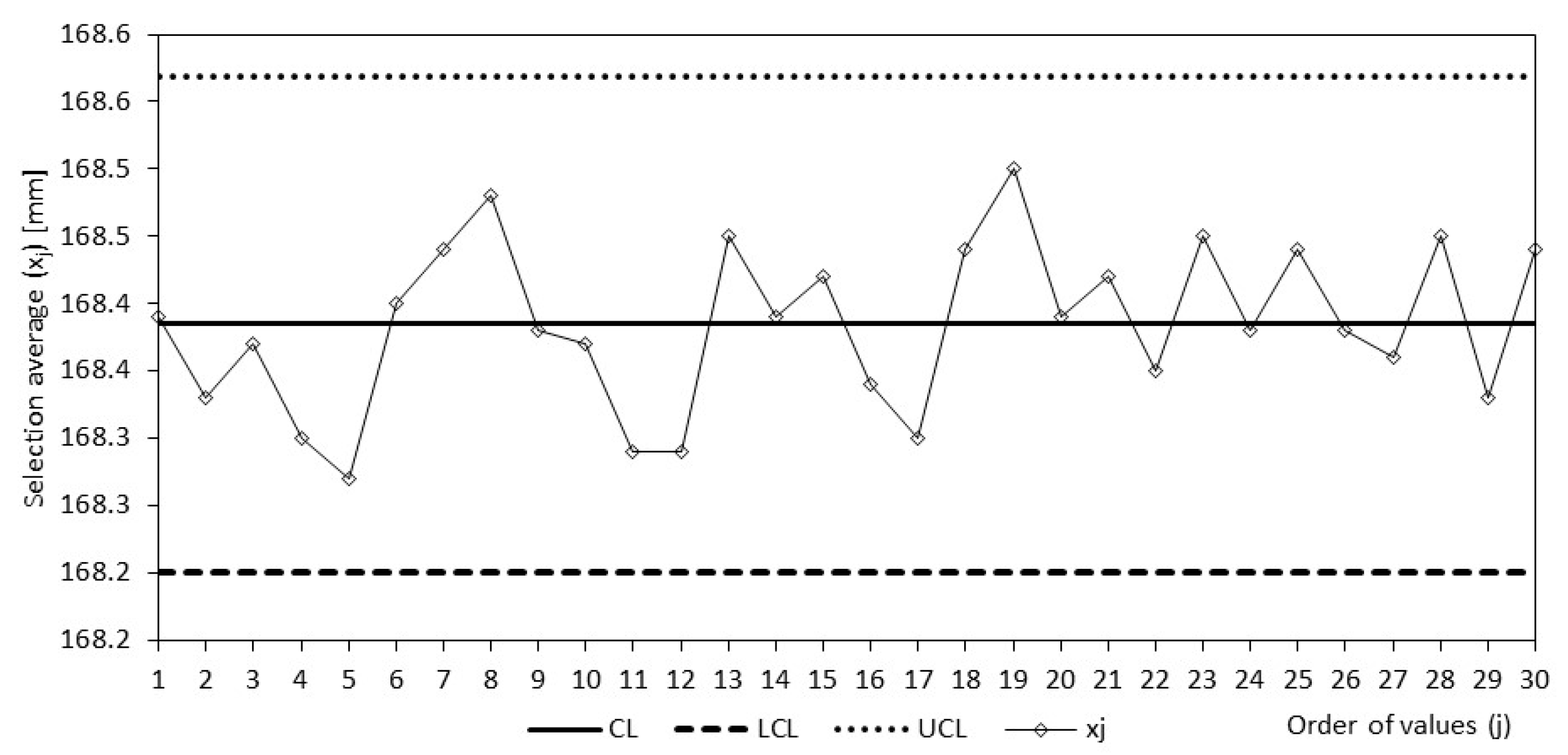
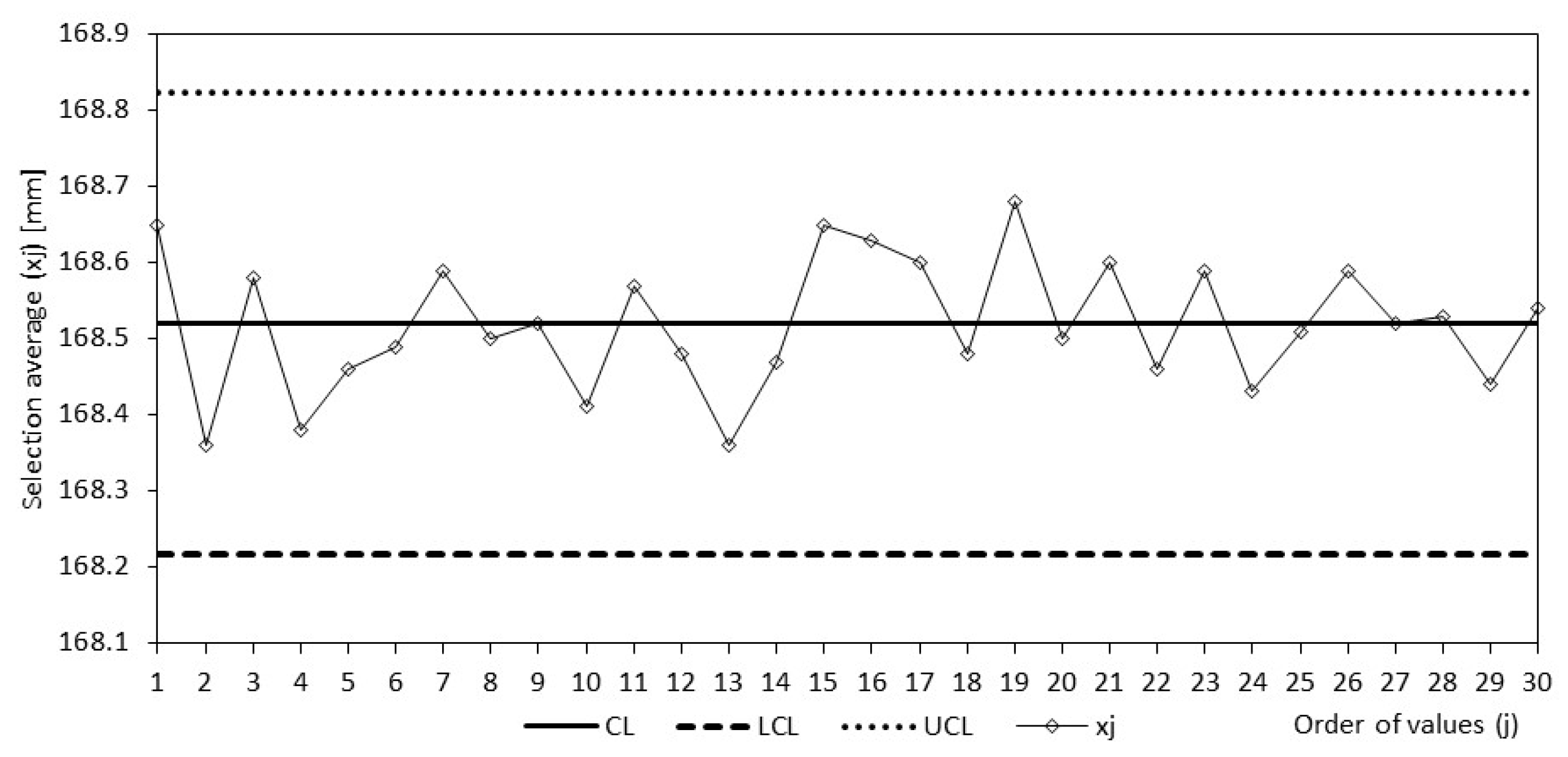
The data used in this paper come from the production of the verification series, but the investigated company subsequently switched to serial production for this product series. In the verification series, three production batches were produced within three days and within one month. The production management identified two critical parameters: the width and length of the product. By implementing Shewhart control diagrams, it was possible to diagnose adverse effects and then take corrective and preventive measures. The purpose of Shewhart’s control diagrams is to obtain information about interventions in the process. Using Shewhart control diagrams, it is possible to achieve and maintain the production process at the required level to ensure the required product parameter compliance. Shewhart control charts indicate problems in the parameter setting of the production process. It is crucial to monitor the variability and maintain the centre values of the respective measurements when setting up the production process. Within the investigated case study scenario, at the beginning of the verification series for parameters “width” and “length”, the findings show that both set parameters did not meet the customer’s requirements. In both cases, measurement errors were evident on the first day of the verification series. This study also confirms that, from the point of view of statistical calculations on the first day of the verification series, the production process needs to be set to specific required parameters. The following measurements show an improvement on the second and third verification days.
Statistical analyses show that the set parameters still need to be met in the first two days of the test series. An improvement in the process is observed on the third day of the test series. Based on the setting and fine-tuning of the parameters in the case of the third day of the test series, it can be concluded that the process is well set, which is confirmed by verifying the stability of the process. An essential condition for setting the control charts is to observe the correct chronological arrangement and regular acquisition of measured values.
Due to inaccuracy and mistakes during the measurements, repeated measurements were necessary. The purpose of managing the smooth running of the production process is to regulate, coordinate and control the production process through management tools and statistical quality control. The current turbulent and dynamically developing environment requires, in addition to compliance with delivery dates, the use of ecologically appropriate materials and technologies and compliance with product quality parameters. On the other hand, it is a complex, laborious and demanding tool; collecting the necessary data and evaluating them objectively and effectively is necessary. The implementation of statistical regulation in the management and control of the production process allows the company’s top management to eliminate the consumption of used material and used energy and reduce the total production costs.
Solving tasks in the future must be oriented toward the evaluation of the capability of the production process of the monitored product. The proposal for the following research will be oriented to evaluating the capability through process capability indices for continuous data using the classical method for Cp, Cpk, Pp, and Ppk and with a set minimum limit of 1.33. Another suggestion for process capability assessment is the calculation of Cpmk and Cpm indices.
This specific and realized research has demonstrated, in the form of a case study of the conditions of a real company, that it can offer that company an advantage due to the quality control of the “width” and “length” parameters. The priority of the organization in the long term is toward an effort to comply with the required parameters “width” and “length” determining the quality of manufactured products. In the case of the increasing variability, this result may have a negative impact on the basic parameters of the product. The implementation of Shewhart’s control diagrams contributes to the elimination or removal of the deformation of plastic mouldings, which in turn leads to ensuring the correct functioning of their related production process. The current modern era requires an increase in the quality parameters of individual production processes, which will ultimately have an impact on the competitiveness of the company and an increase in market share.
Shewhart control charts are useful for identifying deviations that indicate non-compliance with quality limits. The proposed methodological framework was subsequently implemented in a real case study of a company focused on the field of automobile production. The research showed the improvement, innovation and advancement to a higher level, not only in terms of technology but also in compliance with quality parameters in order to satisfy the demands of customers on the market.
Realized Shewhart control diagrams present the measurements taken during test batches while setting up the machines and establishing the process itself. The scientific contribution consists in monitoring and investigating the deformation of plastic mouldings with a connection to the method of statistical quality control. The positive scientific contribution of the application of Shewhart’s control diagrams derives from the way it leads to improved quality and higher efficiency. The everyday reality of the company centres around ensuring the continuous operation of the production process, minimizing non-conforming products and eliminating downtime. Applying these three motivations helps to ensure quality, reduce production line times and eliminate waste.
Ultimately, the company must respond flexibly to change and it is in the company’s interest to prosper and increase its market share. It is the application of Shewhart control diagrams that contributes to the elimination of non-conforming products as well as to the elimination of downtime. Through the application of Shewhart control charts, production of non-conforming products was reduced by 10%. It should be emphasized that the result must have a positive effect on the basic parameters of the product. The current modern era requires the streamlining of production processes by applying Shewhart’s control charts, the application of which has begun to represent a major trend in manufacturing companies. The implementation of Shewhart control charts is aimed at increasing productivity as well as eliminating costs incurred.
The calculation of process capability through process capability indices, namely Cp, Cpk, Cpm, Cpmk and Pp, Ppk will be the subject of further studies. The use of more modern and reliable indices will focus on both variability and on the degree to which the optimal value of the observed quality is achieved in order to achieve further improvement of the results.

Author Contributions

Conceptualization, M.M. and K.Č.; methodology, M.M., J.T. and K.Č.; software, M.M.; validation, K.Č., M.M. and J.T.; formal analysis, K.Č.; investigation, J.T.; resources, M.M.; data curation, K.Č. and J.T.; writing—original draft preparation, K.Č.; writing—review and editing, M.M.; visualization, M.M.; supervision, K.Č., J.T. and M.M.; project administration, K.Č.; funding acquisition, M.M. All authors have read and agreed to the published version of the manuscript.

Funding

This work is supported by the Scientific Grant Agency of the Ministry of Education, Science, Research, and Sport of the Slovak Republic and the Slovak Academy Sciences as part of the research project VEGA 1/0408/23.

Data Availability Statement

Data is unavailable due to privacy.

Conflicts of Interest

The authors declare no conflict of interest.

References

  1. Plastics Europe. Plastics—The Facts 2022. Available online: https://plasticseurope.org/wp-content/uploads/2022/12/PE-PLASTICS-THE-FACTS_FINAL_DIGITAL.pdf (accessed on 20 February 2023).
  2. Flegner, P.; Bogdanovska, G. Drilling tool speed analysis using Shewhart charts. Elektrotechnika Strojárstvo 2013, 6, 1–9. [Google Scholar]
  3. Kisić, E.; Petrović, V.; Jakovljević, M.; Đurović, Z. Fault detection in electric power systems based on control charts. Serb. J. Electr. Eng. 2013, 10, 73–90. [Google Scholar] [CrossRef]
  4. Fu, X.; Wang, R.; Dong, Z. Application of a Shewhart control chart to monitor clean ash during coal preparation. Int. J. Miner. Process. 2017, 158, 45–54. [Google Scholar] [CrossRef]
  5. Berlemann, M.; Freese, J.; Knoth, S. Dating the start of the US house price bubble: An application of statistical process control. J. Empir. Econ. 2019, 58, 2287–2307. [Google Scholar] [CrossRef]
  6. Biswas, R.K.; Masud, M.S.; Kabir, E. Shewhart control chart for individual measurement: An application in a weaving mill. Australas. J. Bus. Soc. Sci. Inf. Technol. 2016, 2, 89–100. [Google Scholar]
  7. Montgomery, D.C. Statistical Quality Control; Wiley Online Library: Hoboken, NJ, USA, 2012; Available online: https://www.oreilly.com/library/view/statistical-quality-control/9781118146811/ (accessed on 14 December 2022).
  8. Zhu, F. Application of Shewhart Control Charts in the inspection of pharmaceutical manufacturing process. Int. J. Pharm. Chem. 2019, 5, 1–11. [Google Scholar] [CrossRef]
  9. Castagliola, P.; Celano, G.; Fichera, S.; Nenes, G. The variable sample size t control chart for monitoring short production runs. Int. J. Adv. Manuf. Technol. 2013, 66, 1353–1366. [Google Scholar] [CrossRef]
  10. Celano, G.; Castagliola, P.; Trovato, E.; Fichera, S. The economic performance of the Shewhart t chart. Qual. Reliab. Eng. Int. 2012, 28, 159–180. [Google Scholar] [CrossRef]
  11. Li, Y.; Pu, X.L. On the performance of two-sided control charts for short production runs. Qual. Reliab. Eng. Int. 2012, 28, 215–232. [Google Scholar] [CrossRef]
  12. Tasias, K.A.; Nenes, G. A variable parameter Shewhart control scheme for joint monitoring of process mean and variance. Comput. Ind. Eng. 2012, 63, 1154–1170. [Google Scholar] [CrossRef]
  13. Bersimis, S.; Psarakis, S.; Panaretos, J. Multivariate statistical process control charts: An overview. Qual. Reliab. Eng. Int. 2007, 23, 517–543. [Google Scholar] [CrossRef]
  14. Zhou, C.L.; Tsung, F. Multivariate sign EWMA control chart. Technometrics 2011, 53, 84–97. [Google Scholar] [CrossRef]
  15. Nenes, G.; Castagliola, P.; Celano, G.; Panagiotidou, S. The variable sampling interval control chart for finite-horizon processes. IIE Trans. 2014, 46, 1050–1065. [Google Scholar] [CrossRef]
  16. Chowdhury, S.; Mukherjee, A.; Chakraborti, S. A new distribution-free control chart for joint monitoring of unknown location and scale parameters of continuous distributions. Qual. Reliab. Eng. Int. 2014, 30, 191–204. [Google Scholar] [CrossRef]
  17. Li, J. Nonparametric multivariate statistical process control charts: A hypothesis testing—Based approach. J. Nonparametric Stat. 2015, 27, 384–400. [Google Scholar] [CrossRef]
  18. Qiu, P. Some perspectives on nonparametric statistical process control. J. Qual. Technol. 2018, 50, 49–65. [Google Scholar] [CrossRef]
  19. Mukherjee, A.; Marozzi, M. Nonparametric phase-II control parts for monitoring high-dimensional processes with unknown parameters. J. Qual. Technol. 2021, 54, 44–64. [Google Scholar] [CrossRef]
  20. Lenfeld, P. Technology II: Plastics Processing; Technická Univerzita Liberec, Fakulta Strojní: Liberec, Czech Republic, 2015; 138p. [Google Scholar]
  21. Beaumont, J.P.; Nagel, R.F.; Sherman, R. Successful Injection Molding; Hanser: Munich, Germany, 2002; 361p. [Google Scholar]
  22. Hluchý, M. Engineering Technologies II: Semi-Finished Products and Their Technological; Scienta: Praha, Czech Republic, 2001; 352p. [Google Scholar]
  23. Trebuna, P.; Straka, M.; Rosova, A.; Malindzakova, M. Petri nets as a tool for production streamlining in plastics processing. Przem. Chem. 2015, 94, 1605–1608. [Google Scholar] [CrossRef]
  24. Andrejiova, M. Statistical Methods in Practise, 1st ed.; Technical University of Kosice: Kosice, Slovakia, 2016; 318p. [Google Scholar]
  25. Kačmáry, P.; Rosová, A.; Straka, M.; Malindzakova, M.; Puškáš, E. Introduction to the combined model of forecasting and its application and comparation with Arima model. In Proceedings of the 6th Carpathian Logistics Congress (CLC 2015), Jesenik, Czech Republic, 4–6 November 2015. [Google Scholar]
  26. Ercole, A.; Raganati, F.; Salatino, P.; Maerzocchella, A. Continuous succinic acid production by immobilized cells of Actinobacillus succinogenes in a fluidized bed reactor: Entrapment in alginate beads. Biochem. Eng. J. 2021, 169, 107968. [Google Scholar] [CrossRef]
  27. Xu, H.; Shi, B. Design and System Evaluation of Mixed Waste Plastic Gasification Process Based on Integrated Gasification Combined Cycle System. Processes 2022, 10, 499. [Google Scholar] [CrossRef]
  28. Anderson, L.; Yu, E.; Chen, W.T. Chemical Recycling of Mixed Plastics in Electronic Waste Using Solvent-Based Processing. Processes 2022, 10, 66. [Google Scholar] [CrossRef]
  29. Sztorch, B.; Brzakalski, D.; Jalbrzykowski, M.; Przekop, R.E. Processing Technologies for Crisis Response on the Example of COVID-19 Pandemic-Injection Molding and FFF Case Study. Processes 2022, 9, 791. [Google Scholar] [CrossRef]
Figure 1. Plastic injection cycle [20].
Processes 11 01246 g001
Figure 2. Methodical frame for the parameter identification of the production stability.
Processes 11 01246 g002
Figure 3. Shewhart control chart.
Processes 11 01246 g003
Figure 4. Measured data for the width parameter, first day.
Processes 11 01246 g004
Figure 5. Histogram and frequency function for the width parameter, first day.
Processes 11 01246 g005
Figure 6. Measured data of the width parameter, second day.
Processes 11 01246 g006
Figure 7. Histogram and the frequency function for the width parameter, second day.
Processes 11 01246 g007
Figure 8. Shewhart control chart for sliding margins for the width parameter, second day.
Processes 11 01246 g008
Figure 9. Shewhart control chart individual values for the width parameter, second day.
Processes 11 01246 g009
Figure 10. Measured data for the width parameter, third day.
Processes 11 01246 g010
Figure 11. Histogram and frequency function for the width parameter, third day.
Processes 11 01246 g011
Figure 12. Shewhart control chart for sliding margins for the width parameter, third day.
Processes 11 01246 g012
Figure 13. Shewhart control chart for individual values for the width parameter, third day.
Processes 11 01246 g013
Figure 14. Measured data for the length parameter, first day [20].
Processes 11 01246 g014
Figure 15. Histogram and frequency function for the length parameter, first day [20].
Processes 11 01246 g015
Figure 16. Measured data for the length parameter, second day [20].
Processes 11 01246 g016
Figure 17. Histogram and the frequency function for the length parameter, second day.
Processes 11 01246 g017
Figure 18. Shewhart control chart for sliding margins for the length parameter, second day.
Processes 11 01246 g018
Figure 19. Shewhart control chart for individual values for the length parameter, second day.
Processes 11 01246 g019
Figure 20. Histogram and the frequency function for the length parameter, third day.
Processes 11 01246 g020
Figure 21. Shewhart control chart for sliding margins for the length parameter, third day.
Processes 11 01246 g021
Figure 22. Shewhart control chart for individual values, parameter length, 3rd day.
Processes 11 01246 g022
Disclaimer/Publisher’s Note: The statements, opinions and data contained in all publications are solely those of the individual author(s) and contributor(s) and not of MDPI and/or the editor(s). MDPI and/or the editor(s) disclaim responsibility for any injury to people or property resulting from any ideas, methods, instructions or products referred to in the content.

