Article

Predictive Control Strategy for Continuous Production Systems: A Comparative Study with Classical Control Approaches Using Simulation-Based Analysis

by
Amelia Chindrus
1,†,
Dana Copot
2,† and
Constantin-Florin Caruntu
1,*,†
1
Department of Automatic Control and Applied Informatics, “Gheorghe Asachi” Technical University of Iasi, 700050 Iasi, Romania
2
Department of Electromechanical, Systems and Metal Engineering, Ghent University, 9000 Ghent, Belgium
*
Author to whom correspondence should be addressed.
These authors contributed equally to this work.
Processes 2023, 11(4), 1258; https://doi.org/10.3390/pr11041258
Submission received: 13 March 2023 / Revised: 11 April 2023 / Accepted: 13 April 2023 / Published: 19 April 2023
(This article belongs to the Section Pharmaceutical Processes)

Abstract

:
Due to today’s technological development and information progress, an increasing number of physical systems have become interconnected and linked together through communication networks, thus resulting in Cyber-Physical Systems (CPSs). Continuous manufacturing, which involves the manufacture of products without interruption, has become increasingly important in many industries, including the pharmaceutical and chemical industries. CPSs can be used to control and monitor the production process, which is essential in enabling continuous manufacturing. This paper is focused on the modeling and control of physical systems required in tablet production using dry granulation. Tablets are a type of oral dosage form that is commonly used in the pharmaceutical industry. They are solid, compressed forms of medication that are formulated to release the active ingredients in a manner that allows for optimal absorption and efficacy. Thus, a model predictive control (MPC) strategy is applied to a plant model to test the designed controller and to analyze the obtained performances. The simulation results are compared with those obtained using other control algorithms, linear quadratic regulator (LQR) and proportional-integral-derivative (PID), applied to the same plant model. The results showed that the predictive control strategy performed significantly better than the other two control strategies.

1. Introduction

Advances in data acquisition systems, information technology (IT), and networking technologies have led to the development of Cyber-Physical Systems (CPSs). These systems are complex infrastructures that integrate digital technology into physical reality in order to automate and digitalize physical processes [1]. Research and advances in CPS technologies have increasingly become part of emerging trends in IT fields such as the Internet of Things [2], Big Data [3], Cloud Computing, and Artificial Intelligence [4]. Cyber-physical systems offer numerous benefits to technology, industries, and organizations. They improve efficiency, productivity, and safety in manufacturing, healthcare, transportation, and other sectors. By integrating physical devices and software systems, cyber-physical systems enable real-time monitoring, analysis, and control of complex processes, resulting in enhanced performance, reduced costs, and better decision-making capabilities. As a result, cyber-physical systems have the potential to revolutionize multiple industries and transform the way organizations operate. In the context of Industry 4.0, next-generation technologies have propelled the development of smart manufacturing due to the many benefits they offer [5]. The economic benefits are among the most important for manufacturers as they can reduce their production costs by reducing manpower due to process automation, increasing production, and reducing raw material losses. Increasing production volume and quality of the yielded products are important factors in the industry’s technological development due to the increasing demand on the market.
Because CPSs use both hardware and software resources to integrate computing, communication, and control processes, they are used in many fields such as automotive, aerospace, transportation, energy, and manufacturing. Among the many applications of CPS is the pharmaceutical industry, which needs to be upgraded due to the increasing demand for products, highlighted during the COVID pandemic.
The first step towards the modernization of industry is the transition to continuous production, necessary for the emergence of smart factories [6]. Continuous production is a production flow method used to manufacture, produce, or process materials without interruption. During continuous processing, materials are transported from one processing unit to another in a continuous flow to produce a finished product. Regardless of the industry in which it is applied, continuous production offers the major advantage of a higher production rate as well as an increased standard of product quality. It also decreases production time, the possibility of human error, and per unit costs, while production flexibility increases and the ability to scale up is improved. This type of process is used by companies involved in oil refining, metal smelting, power plants, sanitary wastewater treatment, and many more. Other industries, such as pharmaceuticals, are beginning to understand the benefits of a continuous production process, whereby products can be manufactured in a shorter time, at the lowest possible cost, while minimizing waste [7].
At the moment, most pharmaceutical companies are focused on batch production because it is cheaper compared to continuous manufacturing (CM) [8]. This approach requires each batch to go through the same steps at the same time. Unlike continuous production, where both raw material and finished product are charged/discharged continuously throughout the process, in batch production, all raw material is charged at the start of the process and the products are discharged at once [9]. This is a disadvantage because quality checks and inspection of products are made on samples from an already manufactured batch, compared to continuous production where products can be inspected in advance at each stage.
Pharmaceutical products can be found in many forms, depending on the purpose of use and how they are administered. Thus, they can be classified into oral (pills/tablets, capsules, syrups, solutions), cutaneous (unguents, gels, creams, solutions), and inhalation (solution, spray) pharmaceutical forms. Depending on the classification of the products, the method of manufacture also differs. This paper is focused on solid dosage forms, in which case the research carried out so far on the continuous production of these types of drugs still requires improvement [8]. In [10], the risks and economics of adopting continuous production for pharmaceutical tablets compared to conventional batch production are presented. The results of the studies demonstrate the potential of CM to make internal production of pharmaceuticals more economically attractive than external production of these products. A case study on the sustainability of using CM in pharmaceutical production is also illustrated in [11]. The examples analyzed in this article show that in most situations there are positive sustainability factors for the use of this method in the manufacturing process of chemical compounds needed for pharmaceutical products.
The transition to continuous manufacturing of pharmaceuticals is supported by a report of the Subcommittee on Advanced Manufacturing, Committee on Technology of the National Science and Technology Council, US, in October 2022 [12], which recommends “advanced continuous manufacturing, in-line process monitoring and control, integrated AI-assisted systems, and novel cell culture techniques".
Solid dosage forms can be classified according to the manufacturing process as follows: direct compression (DC), dry granulation (DG), or wet granulation (WG) [7]. Continuous direct compression includes multiple loss-in-weight feeders, a blender required for mixing active pharmaceutical ingredients (APIs) with powdered excipients, and a rotary tablet press. Optionally, a mill (for grounding ingredients from feeders) and a feeder lubricant can be added before the blender. Additionally, in the case of the WG route, a twin screw granulator is used to grind the primary powder. After that, the dryer reaches the desired moisture level and a mill ensures that the granules are the desired size. In addition to the processing units used in DC, a roller compactor and a mill are required in DG after blending the ingredients. The manufacturing process should be chosen according to the physical properties of the tablets (weight variation, thickness, hardness, diameter) and tablet performance (disintegration and dissolution).
Propelled by market requirements and technological advancement, the pharmaceutical industry is encouraged to adopt continuous manufacturing to increase the efficiency and flexibility of drug production by optimizing costs and production times and enhancing product quality. In this work, the focus is on developing and testing a novel model predictive control strategy for such processes. The proposed algorithm is designed for a simulator (developed in Simulink) of the continuous dry granulation manufacturing process of pharmaceutical tablets. To better illustrate the performance of the proposed strategy, the results obtained from the simulations are compared with those provided by two classical control approaches: PID and LQR. Thus, it can be noticed that MPC provides significantly improved results in terms of stability of the production process and increased quality of the final products.
Considering all the aspects mentioned above, the main contributions of this paper, in comparison with our previous work and the current literature, are the following:
  • A new predictive control strategy, adapted for a continuous pharmaceutical tablet manufacturing plant using dry granulation, was developed.
  • The control performance of the algorithm was tested and analyzed by simulations performed on a benchmark simulator designed based on the models that are available in the literature.
  • A comparison between the results provided by the proposed predictive control strategy and those obtained using PID and LQR algorithms was performed.
In this paper, a particular application, i.e., oral dosage form production in a continuous fashion is used as a study case to test and evaluate the fundamental algorithms that have been developed. The purpose of this paper is to illustrate the advantage of modeling and control techniques in the continuous production of pharmaceuticals. The established methods used in the manufacture of solid dosage forms are compared in Section 2, while Section 3 details the dry granulation process model. In this paper, a predictive control strategy is applied to a novel pilot plant of a tablet manufacturing process, which considers system constraints at the design stage. Section 4 focuses on the control architecture of the system and the predictive control strategy applied to the process. The method proposed in the current paper has significant improvements, which will be illustrated and compared with other control strategies in Section 5. The conclusions of these results and future directions of work are presented in Section 6.

2. Direct Compression vs. Dry/Wet Granulation

Either dry granulation (DG) or wet granulation (WG), the use of a granulation method in tablet manufacture is preferable due to the issues of poor fluidity, segregation, and content uniformity. The main advantages of DG compared to WG are the simplified operating process and the absence of the additional energy-consuming drying step. DG is also suitable for processing temperature-sensitive and easily hydrolyzed compounds [13].
In batch production, direct compression (DC) is considered a risky method mainly due to the risk of segregation of the mixture. Therefore, formulations that tend to segregate are often granulated to ensure consistent uniformity of active ingredients contained in the final product. However, it has been observed that when production is performed in a continuous mode, even using DC, increased homogeneity can be achieved for products with high segregation tendencies due to the minimization of internal gaps and elimination of semi-continuous steps [14]. The strong tendency of APIs to agglomerate is a strong argument for the use of granulation in batch manufacturing. This problem is completely solved by the use of a properly designed continuous system in which the material lacks the time and the environment to re-agglomerate [15]. Compared to DC and DG, WG is one of the most difficult pharmaceutical processes to model due to the increased number of steps and variables used in system design [13].
In terms of scale-up, the feasibility of direct compression is negatively influenced due to speed-sensitive compactibility or flow limitations compared to WG. Dry granulation based on roller compaction increases density and flow [16]. The simplicity of the DC process compared with (dry/wet) granulation reduces the complexity, risks, and costs of processing materials. Technically, any additional operations introduced by the granulation process come with validation, yield, cleaning, and documentation issues, in addition to time and effort issues in high-cost good manufacturing practice (GMP) containment facilities [15]. In addition, the heat and humidity problems that can occur in WG may be unacceptable for labile active substances [16]. In direct compression, product quality and consistency are essential, an advantage offered by the possibility of direct expression of input material properties [16]. However, the simplicity of the DC process requires additional constraints on the formulation components compared to production processes involving granulation [17].
Another aspect of the differences between the three routes of manufacture of tablets is the coloring of the tablets. DC and DG are unable to provide the same color intensity compared to WG [18]. In dry granulation, the powder mixture is compressed into granules without the use of a liquid binder. Since no liquid is added to the mixture, the risk of color variations due to moisture or reaction with the binder is minimized, but in its absence, the resulting mixture may have an inconsistent distribution of colorants in the final tablets. Wet granulation involves the addition of a liquid binder to the powder mixture, which can help to distribute the colorant evenly throughout the granules. In the case of direct compression, the homogeneity of the mixture can be more challenging to achieve, which can result in uneven distribution of the colorant in the final tablets.
In [16], the case of sodium starch glycolate is exemplified whose insolubility property does not exclude incompatibilities associated with sodium salts, especially in the presence of moisture. The reaction rate of the finished product is directly proportional to the water activity in it. In this situation, it is not recommended to use DC and DG methods because water activity is probably inhomogeneous in the tablet matrix and local microambitates with high water activity may exist. Another concrete example also illustrated in [16] is for vitamin tablets for which both WG and DG are used. However, in this case, it is recommended to use the DG method which offers a higher yield and more stable products due to the removal of water.
A summary of the advantages/disadvantages of the three production routes for pharmaceutical tablets is presented in Table 1.

3. Process Description

In the context of Cyber-Physical Systems, the pharmaceutical industry needs to take a new approach to the manufacturing process. Currently, the manufacturing process is performed in batches, where the materials are stored before being sent to the next processing stage and their quality is tested off the production line [9]. In the case of continuous manufacturing, the products obtained in each stage are sent directly to the next processing unit. Thus, the design of a continuous manufacturing system involves a complex control strategy to ensure the required quality standards, as well as proper process control. All this is then quantified in increased productivity and reduced production and manufacturing times. Continuous production, unlike batch production, is a flow production strategy. This means that the process never stops, and there are no breaks between the different steps of product creation.

3.1. Process Structure

Before being released for distribution and consumption, tablets are subjected to quality tests, such as the content of active ingredient test, weight uniformity test, dissolution test, or hardness test. The most common defects in compressing table processes are weight variation, low hardness/low mechanical strength of tablets, poor mixing, or layered tablet splitting [21].
For tablet manufacturing, the most common processes are wet granulation, direct compression, or dry granulation. The first two continuous manufacturing methods are shown in Figure 1, where, with red, the route of wet granulation is exemplified and, with green, the route via direct compaction.
This work is focused on the dry granulation process of tablets, modeled in Matlab-Simulink [22]. The model designed for the process considered in this paper is based on numerical data found in the literature. The main execution elements included in the designed model are the feeders for active pharmaceutical ingredients and excipients, the blender and the hoppers associated with the roller compactor (RC) and tablet press (TP). Figure 2 shows the order of the production steps and the dependencies between the processing units. As shown in the above-mentioned figure, the feeders of dry ingredients are connected to a continuous blender that mixes all these ingredients. This results in a powder mixture that feeds a roller compactor that converts the powder blend into the ribbon. A mill is integrated with the roller compactor that breaks down the ribbon and forms granules. These granules are fed to the tablet press via a rotary feed frame. The powder blend fills a die and is subsequently compressed to create a tablet; after compaction, the tablets are coated [23].

3.2. Process Modelling

The main purpose of the unit operation of feeding is to be able to supply APIs, excipients, and lubricants to the next unit, considering a certain constant flow rate, to match the desired mixture composition and total material flow rate. For the considered continuous process, the screw feeder is mostly used. It consists of a feed hopper, one (or more) bridge-breaking systems, and a single (or twin) configuration of conveying screws through which material is distributed out of the unit [24]. The great advantage of this type of power supply is the ability to manage very low flow rates, providing good accuracy. In this operation, an important parameter is the feed factor, which is defined as the amount of powder present in a screw pitch at each rotation of the feed screw. It can be calculated as follows:
f f = m ˙ ω ,
where m ˙ is the mass flow rate and ω is the screw speed.
Note that, the weight in the feeder hopper is assumed to be constant. Using Heckel’s equation [25], the changes in density inside the feeder unit are characterized as:
ρ f e e d i n g ( W ) = ρ m a x ( ρ m a x ρ m i n ) e K W g A f e e d e r ,
where W is the weight of the material inside the feeder, ρ f e e d i n g is the perceived density that is present at the inlet of the screw, ρ m a x is the density at which the perceived density remains constant while more materials are being added to the feeder, q m i n is the minimum density and occurs when W 0 , meaning that the feeder is nearly empty, K is the modified pressure decay constant, g is the gravity acceleration, and A f e e d e r is the cross-sectional area of the feeder.
Since the density is linked with the feed factor, it can be used to characterize this as well. In [26,27], a feed factor model based on Heckel’s equation was developed and analyzed, in the following form:
f f a p a r e n t ( W ) = f f m a x ( f f m a x f f m i n ) e β W ,
where f f m a x corresponds to the maximum relative bulk density within the screws, and f f m i n is the minimum relative bulk density or powder compressibility within the screws. The constant parameter β inside the exponential represents the rate at which the amount of powder present in the screw pitch decreases with respect to a decrease in feeder weight [28] and is defined as:
β = K g A f e e d e r .
In order to capture the feed factor variability that is a consequence of the noise, a feed factor noise term is added to Equation (3), resulting in:
f f ( W ) = f f a p a r e n t + f f v a r .
A truncated cosine Fourier series is used to realize this variability and the following equation results:
f f v a r ( W ) = j = 1 3 A j cos ( W P j ) ,
where A j and P j are constant material dependent parameters.
The blender unit guarantees uniformity of concentration and homogenization. The construction of the mathematical model for a continuous blending process is based on the population equation [29]:
F ( x , t ) t + x F ( x , t ) d x d t = R f o r m ( x , t ) R d e p ( x , t ) + F ˙ i n ( x , t ) F ˙ o u t ( x , t ) ,
where F is the population distribution function, x is the vector of internal coordinates used to express the particle size and t is the time. R f o r m and R d e p indicate the particles that are formed and depleted, respectively, while F ˙ i n and F ˙ o u t are the rates at which the components are fed/neglected to/by the system.
Due to the complexity of the system and the lack of numerical parameters, the blender has been divided into several compartments. These local homogeneous compartments are created by discretizing the mixing vessel space in both axial and radial dimensions. Applying Equation (7) to the process under consideration results in a simple mass balance of a compartment containing the powder flows:
m i , j t = F f [ m i 1 , j m i , j ] + F b [ m i + 1 , j m i , j ] + F r [ m i , j + 1 + m i , j 1 m i , j ] ,
where m i , j is the mass holdup in the compartment and the forward ( F f ) , backward ( F b ) , and radial ( F r ) fluxes are obtained using:
F f = a ω b l e n d e r + b , F b = c ω b l e n d e r + d , F r = e ,
in which ω b l e n d e r is the speed of the blender, while constant parameters a , b (for forward flux), c , d (for backward flux), and e (for radial flux) are estimated from experimental data, depending on the type of material (API or excipient).
Considering the following definition for the flow at the outlet of the blender:
F b l e n d e r = j = 1 N r F f , A P I m A P I , i = N a , j + j = 1 N r F f , E x c i p i e n t m E x c i p i e n t , i = N a , j ,
where m A P I and m E x c i p i e n t are the powder holdups of the last compartments in the axial direction, N r represents the number of radial discretization, and N a is the number of axial compartments, the outlet concentration ( C A P I ) is resolved:
C A P I = j = 1 N r F f , A P I m A P I , i = N a , j F b l e n d e r .
The RC hopper and the TP hopper used in this paper are working on the same principle. The hoppers modeled in this work consist of a conical section at the bottom and a cylindrical section at the top. The hopper model described below will finally provide the resulting height and mass flow rate. In steady-state, the mass flow through all units is the same. Thus, both hoppers will operate under the same operating conditions. This fact causes a delay in the density coming from the previous unit (blender or roller compactor).
The powder that leaves the blender comes into a hopper as well as the material that exits the roller compactor [22]. This unit is modeled as a conical, spherical hopper-type tank. The dynamics of the system are guided by the mass balance equation, defined as the difference between the inlet mass flow rate that is coming from the blender ( m ˙ i n ) and the outlet mass flow rate ( m ˙ o u t ) :
ρ b d V d t = m ˙ i n m ˙ o u t ,
where ρ b is the density at the outlet of the hopper and V is the volume of material in the hopper.
The dynamics of the hopper are modeled by the change in volume in the hopper, depending on the powder’s height:
h < H 1 : d V d t = 1 3 π R 2 H 1 h 2 + R 1 R 2 H 1 h + R 1 2 d h d t , h H 1 : d V d t = π R 2 2 d h d t ,
where R 1 is the radius of the conic section in the bottom and R 2 is the radius of the cylindrical section at the top of the hopper, h is the height of the powder in the hopper and H 1 is the height of the considered section.
The roller compaction process involves turning a powder mixture into a ribbon using a set of counter-rotating rolls that will compress the material. When the particles are fed to the rolls, they are initially considered to be in the slip region of the process [30]. The nip region is the area where the rollers are closest together. The last area, namely the release region, is where the ribbon is already released from the rolls and transported forward. This process is a complex one, depending on a high number of parameters and operating conditions.
An important parameter in this model is the nip angle, defined as the angular position ( θ = α ) , at which the material transforms from slip to non-slip conditions. It depends only on material-related parameters and the following equation is used to calculate it:
4 π 2 α ν tan δ E cot ( B μ ) cot ( B + μ ) = K 2 cos α 1 h 0 R tan α cos α ,
where ν is a variable calculated in relation to the effective angle of friction ( δ E ) and the angle of wall friction, K is the compressibility factor, h 0 is half of the roll gap width, and R is the radius of the roll. The variables B and μ are calculated as:
B = α + μ + π 2 2 , μ = π 4 δ E 2 .
In the nip region, the compression behavior can be calculated using an empirical model, σ = C 1 ρ K , where σ is the material stress and ρ is the compact density, while C 1 is the pre-exponential coefficient of material compression.
Based on Johanson’s model [31] and mass balance equation, the roller compactor model is computed using the compact density at the exit point ( ρ e x i t ) and the inlet density ( ρ i n ) :
0 θ i n ρ ( θ ) cos θ d θ = 0 a ρ ( θ ) cos θ d θ nip region + a θ i n ρ ( θ ) cos θ d θ slip region = = ρ e x i t h 0 R 2 1 + h 0 R h 0 R 2 + h 0 R arctan 1 + 2 R h 0 tan α 2 α + ρ i n ( cos ν sin α ) .
In Equation (15), ρ i n is a variable equal to π / 2 ν and ρ ( θ ) is density profile, relative to angular position θ . Finally, the outlet mass flow rate can be calculated, m ˙ o u t = R W h W ρ e x i t , where W is the roll width and h = 2 h 0 .
The tableting process involves compacting powder mixtures to form a solid dosage form. The performance of tableting processes can be assessed based on tablet active ingredient content, content uniformity, weight variability, and physical properties such as friability, hardness, and dissolution performance [30]. In this paper, the final goal of the design of the tableting process model is to obtain the tablet’s hardness and the mass flow out of the tablet. For the first requirement, the pre-compression ( C _ P p r e ) and main compression ( C _ P m a i n ) pressures are formulated based on the Kawakita equation [32]:
C _ P p r e = V 0 V p r e b p r e V 0 ϵ 0 + 1 + V p r e , C _ P m a i n = V p r e V t a b l e t b m a i n V p r e ϵ m a i n + 1 + V t a b l e t ,
where b p r e and b m a i n are material dependent parameters. In the following equations, the required volumes ( V t a b l e t for the volume of the tablet, pre-compression volume V p r e and the feed volume V 0 ) are defined:
V t a b l e t = L t a b l e t A t a b l e t , V p r e = L p r e A t a b l e t , V 0 = L d e p t h A t a b l e t ,
where L t a b l e t , L p r e and L d e p t h are the heights of the tablet, of the powder in the die, and of the powder after compression in the die, respectively, while A t a b l e t represents the area of the tablet. It is notable that, in the considered process model, the pre-compression and main compression forces are calculated as multiplication by 10 6 of the associated pressures.
Finally, the hardness of the tablet is obtained as follows:
H t a b l e t = H m a x 1 e ( 1 ϵ 0 ) V 0 V t a b l e t ρ r c + log 1 ( 1 ϵ 0 ) V 0 ( 14 ρ r c ) V t a b l e t ,
where maximum tablet hardness ( H m a x ) and critical relative density ( ρ r c ) are known variables.
In the case of the mass flow out of the tablet press, this is determined as the product of the production rate ( R t a b l e t ) and the mass of a single tablet ( m t a b l e t ) : m ˙ = R t a b l e t m t a b l e t , where R t a b l e t = T t u r r e t n d i e 60 , considering the speed of the turret T t u r r e t and the number of dies on the turret n d i e .

4. Closed-Loop Control System Framework

As the manufacturing processes of tablets is a complex system, the need for advanced control systems grows increasingly important. To achieve the desired product quality and consistency, closed-loop control systems have been widely adopted in dry granulation processes. The use of closed-loop control systems allows for the real-time monitoring and adjustment of process parameters to ensure the final product meets the required specifications.

4.1. Control System Architecture

The process described in the previous section is modeled in Matlab as a plant, which is the 8 × 8 input-output system presented in Figure 3. The nominal values (Value) of these variables and the associated constraints (lower bounds—LB and upper bounds—UB) are given in Table 2 and Table 3.
The two tables are divided into three sections, indicated by the white and gray regions. The output of each section is influenced by the inputs it receives. These three sections are internally connected through density, and it is essential that the mass flow rate is equal across all three parts: m ˙ b l e n d e r = m ˙ o u t , R C = m ˙ T P .
The architecture for the implementation of the predictive control strategy is resumed in Figure 4, where the Plant block is illustrated in Figure 3 with 8 inputs (manipulated by the MPC controller) and 8 outputs. A centralized control solution involving a single MPC controller was used to manage all processing units involved in the continuous dry granulation process for the manufacture of solid dosage forms.

4.2. Model Predictive Control Strategy

Starting from a linear discrete-time system with m states, n inputs, and p outputs described by the state-space equation in Equation (19), the state x d m , control input u d n and output y d p vectors of the system at discrete time t are defined:
x d [ t + 1 ] = A d x d [ t ] + B d u d [ t ] , y d [ t ] = C d x d [ t ] + D d u d [ t ] ,
where A d m × m , B d m × n , C d p × m , D d p × n are the discretized system matrices obtained using a specified sampling time T s .
Supposing that the matrix pairs ( A d , B d ) and ( C d , A d ) are stabilizable and detectable, respectively, the goal is to find a state-feedback control law, expressed based on the model predictive control law gain K M P C , of the form:
u d [ t ] = K M P C x [ t ] ,
so that the origin of the closed-loop system x d [ t + 1 ] = ( A d + B d K M P C ) x d [ t ] is globally asymptotically stable, which implies that the matrix ( A d + B d K M P C ) is stable.
Thus, the predicted state can be written in matrix form as X ^ [ t ] = M x [ t ] + C U [ t ] [33,34,35], considering the following:
U [ t ] = u [ t | t ] u [ t + 1 | t ] u [ t + h p 1 | t ] ,
with u [ t + i | t ] , i = 0 , , h p 1 , represents the future control sequence with h p the prediction horizon,
X ^ [ t ] = x ^ [ t + 1 | t ] x ^ [ t + 2 | t ] x ^ [ t + h p | t ] ,
where x ^ [ t + i | t ] is the predicted value of the state vector x [ t + i + 1 | t ] = A d x ^ [ t + i | t ] + B d u [ t + i | t ] , i = 0 , 1 , 2 , with the initial condition described by x ^ [ t | t ] = x [ t ] ,
M = A d A d 2 A d h p , C = B d 0 0 A d B d B d 0 A d h p 1 B d A d h p 2 B d B d .
To design an optimal predictive control law expressed as:
U * [ t ] = arg min U J M P C [ t ] ,
it is necessary to minimize a quadratic cost function of the following form:
J M P C [ t ] = U 0 T [ t ] H U 0 [ t ] + 2 U 0 T [ t ] F x 0 [ t ] + x 0 T [ t ] G x 0 [ t ] ,
with
U 0 [ t ] = U [ t ] U s s [ t ] , x 0 [ t ] = x [ t ] x s s [ t ] , H = C T Q ˜ M P C C + R ˜ M P C , F = C T Q ˜ M P C M , G = M T Q ˜ M P C M + Q M P C ,
where at discrete-time instant t, U s s [ t ] and x s s [ t ] correspond to the steady-state values determined from a given reference. The matrices Q ˜ M P C and R ˜ M P C are defined as:
Q ˜ M P C = Q M P C 0 0 0 Q M P C 0 0 0 Q ¯ M P C , R ˜ M P C = R M P C 0 0 0 R M P C 0 0 0 R M P C .
The matrices Q M P C , R M P C , and Q ¯ M P C are positive definite matrices, with Q M P C possibly being positive semi-definite. These matrices are utilized to weigh the states, inputs, and terminal state appropriately.
Assuming there are no constraints, the optimization problem can be solved offline to obtain U * [ t ] = H 1 F z [ t ] and in line with the receding horizon principle, only the initial control command in U * is implemented on the system, as described by u [ t ] = u * [ t | t ] = K M P C x [ t ] , with K M P C = I h p 0 0 H 1 F .
In practical applications, system variables, such as inputs, outputs, and states, are limited by physical constraints, which can include input constraints (actuator limits) or state/output constraints (that can be active during transients or in steady-state). Predictive controllers offer a significant benefit in that they can determine an optimal nonlinear control law for systems with state, input, and/or output constraints in real-time at each sampling period.
The constraints on system variables appear usually due to physical limitations and can be expressed as linear inequalities, which are defined as:
u m i n u [ t ] u m a x x m i n x [ t ] x m a x y m i n y [ t ] y m a x .
Given the quadratic cost function J M P C [ t ] defined in Equation (25) and the constraints specified earlier, the minimization of the cost function involves solving a quadratic problem, which is expressed as [33,34,35]: min U U T H U + 2 x T [ t ] F T U , subject to the constraints that were previously stated.

5. Simulation Results

In this section, the MPC methodology proposed for continuous manufacturing of solid dosage forms using the dry granulation route is tested and compared by simulation with other classical control approaches (described in Section 5.2) applied to the same simulation setup presented in Section 5.1. The obtained illustrative results are presented in Section 5.3 and are completed by numerical analysis in Section 5.4.

5.1. Simulation Setup

The Matlab-Simulink environment was used to model and control the continuous dry granulation tablet production process described in Section 3. A benchmark simulator is created to evaluate the feasibility of developing control strategies that are intended to control the real physical plant. The simulator considered in this work consists of a feeder, a blender, a roller compactor with an RC hopper, a co-mill, and a tablet press with a TP hopper. The Simulink implementation of the fixed part involves a complex system where each processing unit mentioned previously is modeled individually.
This study simulates a powder mixture consisting of API and excipient material. The excipients and APIs feeders get the input speed of the associated screws and provide the respective flow rates at the output. It should be noted that all parameters of the feed factor model used in this work are material dependent. The material properties that have an impact on the feeder performance are: conditioned bulk density, compressibility, permeability, cohesion, flow function coefficient, and the angle of internal friction. The blender is a crucial unit in the pharmaceutical industry since it guarantees concentration uniformity and homogeneity. Several modeling techniques are being used to simulate the dynamics of the powder in the blender. The outputs of the feeders model and the speed of the blender are required for the blender model to provide the outlet concentration, the relative standard deviation as well as the mass flow and the density at the outlet of the blender. In the case of the roller compactor, the key operating variables are the feed speed, roll speed, roll pressure, and the gap between the rolls. The gap and the roller force—the actively controlled process parameters—are the inputs for the model, whereas the screw speed—the changing process parameter—is neglected. The throughput can be predicted once the ribbon density is known. The auger filling may fluctuate from one revolution to another. This fluctuation is modeled by introducing a disturbance in the inlet bulk density. Hereafter, the co-mill is designed based on the outlet density and the outlet mass flow rate from the RC with the co-mill speed. This model will provide the necessary inputs to the hopper associated with the tablet press which is modeled similarly to that of the roller compactor. Finally, the tablet press involves a complex model where it is necessary to have the powder solid density determined previously, turret speed, feed volume, and thickness of the tablet to establish the tablet’s rate, hardness, and mass of the tablet.

5.2. Comparison Control Strategies

Two control strategies, Proportional-Integral-Derivative (PID) [22] and Linear Quadratic Regulator (LQR) [36], are presented and applied to the same simulator to analyze and compare the performance of the proposed strategy for end-to-end continuous pharmaceutical production. PID controllers have been designed for the individual control of the process units involved in the manufacturing process, while for the LQR-based strategy has been proposed a unitary control strategy for the entire process, using a single controller, which is adapted to the system requirements.
Decentralized control strategies offer an alternative to simplify the control of multiple-input multiple-output (MIMO) processes by decomposing the complex system into a series of single-input single-output (SISO) subsystems [37]. However, decentralized control systems have become increasingly popular due to their ability to handle large-scale systems with multiple loops. In such systems, each loop has its own controller, and decisions are made independently of other loops. In [38], a novel approach to designing decentralized controllers based on nonlinear optimization, with the aim of minimizing the impact of disturbances in coupled loops. The proposed methodology achieves improved control performance by taking into account the interdependence between loops and optimizing the control gains for each individual loop.
Figure 5 illustrates the decentralized control strategy applied to the system in which one or more PID controllers are designed for each processing unit involved in the continuous tablet production process, as detailed in Section 5.2.1.
As in the case of predictive control, a centralized control strategy was also applied in the case of LQR, as can be observed in Figure 6, where the Plant block is illustrated in Figure 3 with 8 inputs (manipulated by the LQR controller) and 8 outputs. In addition, an observer has been employed to estimate the system’s unknown states, thereby expanding the control architecture, as detailed in Section 5.2.2.

5.2.1. Proportional-Integral-Derivative Controller

A PID controller is a control loop feedback algorithm used to automatically adjust an output variable based on an input variable and a set point. Thus, it calculates the error as the difference between the desired output and the system’s response. This type of controller is widely used in industrial control systems due to its robust performance and functional simplicity. Several elements can degrade PID controller performance, such as process interactions, process dead time, non-linearity, and process constraints [39]. The control function is defined as the sum of the proportional ( P ) , integral ( I ) , andderivative ( D ) terms [40]:
u [ t ] = P [ t ] + I [ t ] + D [ t ] ,
with
P [ t ] = K p e [ t ] , I [ t ] = K i 0 t e [ τ ] d τ , D [ t ] = K d d d t e [ t ] ,
where K p , i , d is the proportional/integral/derivative gain, e represents the tracking error at time t and τ is the variable of integration.
Tuning the parameters means adjusting the values of the gains to achieve optimal control system performance. In this context, two tuning methods were applied to the simulator, specifically the Frequency Response tool (FRtool), which is a controller design tool, and an optimization-based method (Integral of Time Absolute Error).
FRtool [41] is a program that allows a graphical design of the controller. It is able to tackle systems with time-delays, which is not the case when using the standard Matlab controller design tool, since it operates with frequency diagrams (Nichols charts). The dead time present in the system is not approximated and is treated in the right way.
The Integral of Time Absolute Error (ITAE) [42] is one of the possible criteria of an optimization tuning method. The method involves analytically calculating the gain of the controller ( K p ) , integral time ( K i ) , and the derivative time ( K d ) for PID-controlled systems. A Matlab program is used to find the optimum values for the PID controller to achieve the best performance to satisfy the system requirements: reducing the overshoot, achieving a good load disturbance rejection, and maintaining a high system response. The corresponding objective function is defined as follows:
I T A E = 0 t | e [ t ] | d t ,
where t is the time and e [ t ] is the difference between set point and controlled variable.
Since the dry granulation route consists of three parts (feeder + blender, roller compactor, and tablet press), the evaluation will also be done three ways. So, after comparing the different control strategies and tuning methods in the first part (feeder + blender), the best one will be taken to evaluate the second one. The same will be done for the third part.
In the discussion of the first part, the best structure for the feedforward will be chosen first based on the evaluation, which is used in the other parts as well. In the first part of the granulation route, the cascade control strategy combined with a static feedforward structure, where the PID controllers were tuned using the FRtool, performed better. It was compared to open-loop, only cascade, and other feedforward structures. This output will be fed into the next unit, i.e., the roller compactor (part II of the dry granulation route). Next up is the evaluation of the control strategy for the roller compactor. In this case, the ITAE tuning method is preferred with the feedback combined with feedforward as control strategy. This strategy performs very well and keeps the output variables within the control bounds. This result (part I tuned with FRtool consisting of cascade feedback and feedforward control as a control strategy, part II tuned using the ITAE optimization method consisting of feedback/feedforward control as control strategy) is now used to be fed into the third and last part of the dry granulation route (i.e., the tablet press). The same conclusions as in part II can be drawn, specifically that the combined feedback and feedforward (static structure) control strategy is the most effective.

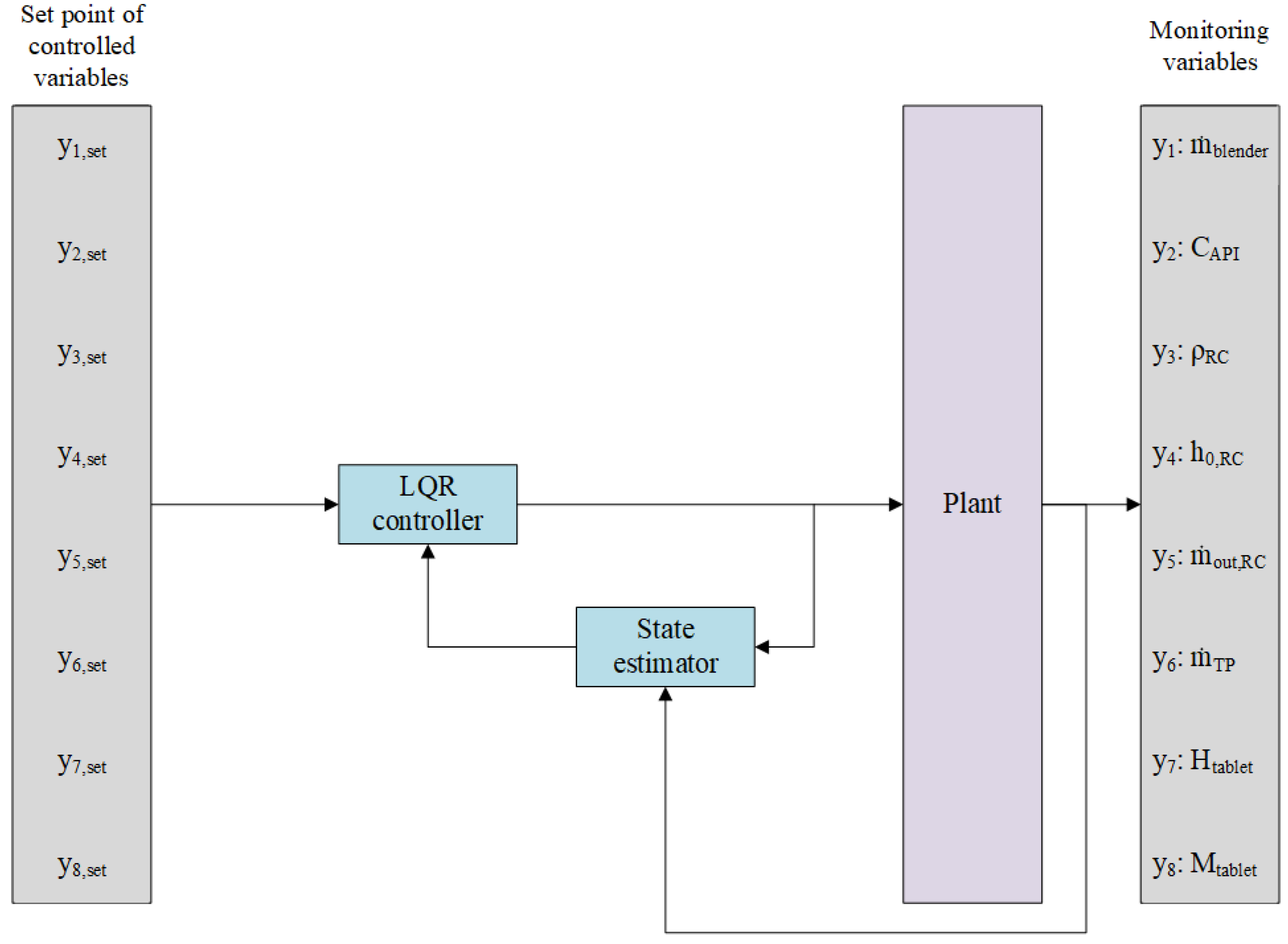
5.2.2. Linear Quadratic Regulator

The LQR control algorithm [43] is based on the state-space model of the process and can handle multiple feedback variables. This leads to a more robust control algorithm as there is more information about the system available. The approach is based on minimizing a quadratic cost function [44] and can be extended to Linear Quadratic Integral control (LQI) or Linear Quadratic Gaussian regulator (LQG).
A control structure with state feedback is implemented using a mathematical model in matrix form (19). The purpose is to find an optimal state-variable feedback control law, which guarantees the desired closed-loop performances and is defined as:
u d [ t ] = K L Q R x d [ t ] ,
where K L Q R is the state feedback gain. Also, a quadratic cost function J L Q R is defined to quantify the controller performance and to design the optimal state-variable feedback gain [44]:
J L Q R = t = 0 { x d T [ t ] Q L Q R x d [ t ] + u d T [ t ] R L Q R u d [ t ] + 2 x d T [ t ] N L Q R u d [ t ] } ,
where the weighting parameters, Q L Q R and N L Q R represent semi-positive definite symmetric matrices of dimension ( m × m ) and R L Q R is a positive definite symmetric matrix of dimension ( n × n ) . To ensure efficient control of each state of the system with minimum effort, as per the aforementioned performance index, it is necessary to select appropriate weight matrices Q L Q R and R L Q R , which determine the closed-loop performance.
Optimizing the performance index J L Q R and solving for K L Q R implies the solution P L Q R of the Discrete Algebraic Riccati Equation [45]:
P L Q R = Q L Q R + A d T P L Q R A d ( A d T P L Q R B d + N L Q R ) ( B d T P L Q R B d + R L Q R ) 1 ( B d T P L Q R A d + N L Q R T ) .
By iteratively solving the Riccati equation of the related matrix, the optimal feedback gain can be achieved:
K L Q R = ( B d T P L Q R B d + R L Q R ) 1 ( B d T P L Q R A d + N L Q R T ) .
In order to achieve the best performance of feedback control, an integral feedback control strategy is used to account for disturbances and noises from the external environment. This is achieved by designing a Linear Quadratic Regulator with Integral action (LQI), which provides zero steady-state error using an integrator. Thus, the Linear Quadratic Regulator with Integral action [46] is designed to provide zero steady-state error using an integrator, added as an additional state ( x i ) to the state vector ( x d ) . This represents the integral of the error between the desired output r, and the actual output y d . Thus, the extended state vector is given as:
x e = x d x i ,
where x i [ t + 1 ] = x i [ t ] + T s ( r [ t ] y d [ t ] ) , with sampling time T s .
The optimal gain matrix K L Q I required to determine the control law given by u i [ t ] = K L Q I x e is obtained similarly to the method presented above.
When the full state variable x d [ t ] cannot be measured in the implementation of a controller, an observer is typically used. The Luenberger observer [47] employs a correction term based on the measured output y d and its estimate y ^ d to model the current system. Assuming observability of the pair ( A d , C d ) in the discretized system from Euqation (19), a full-order observer can be expressed using the following equation [35]:
x ^ d [ t + 1 ] = A d x ^ d [ t ] + B d u d [ t ] + K o b s ( y d [ t ] y ^ d [ t ] ) y ^ d = C d x ^ d ,
where K o b s is the constant observer gain matrix. A conventional method used to model the observer is pole assignment, whereby the selection of gain matrix K o b s can result in various states for the system ( A d , C d ) . If K o b s is chosen to place the eigenvalues of A d K o b s C d at any desired locations in the plane, then the system can be fully observed. The observer is designed with the goal of estimating the actual state x d [ t ] . Based on the definition of the estimation error:
e d [ t ] = x d [ t ] x ^ d [ t ] ,
the observer dynamics lead to the following equation for the estimation error:
e d [ t + 1 ] = x d [ t + 1 ] x ^ d [ t + 1 ] = ( A d K o b s C d ) e d [ t ] .

5.3. Illustrative Results

This section will review the performance of the controlled tablet manufacturing process using a predictive control strategy, which was implemented using the Model Predictive Control Toolbox for Matlab/Simulink, in comparison to the results obtained in [22] using PID, as well as those based on LQR in [36]. Both the performance of disturbance rejection and set-point tracking are analyzed and discussed. The comparative results obtained from the simulations are shown in Figure 7, Figure 8, Figure 9, Figure 10, Figure 11, Figure 12, Figure 13, Figure 14, Figure 15 and Figure 16. The time interval [ 0 , 500 ] s is considered the time until the system sets up and reaches a normal operating mode. Thus, the variations of the signal occurring in this interval do not impact the performance of the proposed strategy.
Defining specific boundaries is essential to assess the efficacy of the control strategy. To evaluate the performance of the controller, upper and lower limits are established for the controlled variables, according to the numerical values presented in Table 3. These values are plotted on the graphs in Figure 7, Figure 8 and Figure 9, Figure 11 and Figure 13, Figure 14, Figure 15 and Figure 16 with red dashed lines. If the controlled variable remains within these predetermined boundaries, it can be concluded that the controller is performing well, the yielded control law, i.e., the manipulated variable, being feasible.
The control inputs of the associated outputs were represented in order to evaluate the performance of the proposed control strategy. The speed of the excipient feeder (Figure 7) is paired with the mass flow rate at the outlet of the blender (Figure 8). The speed of the API feeder (Figure 9) required to provide the concentration at the outlet of the blender (Figure 11Figure 12) can be observed in detail in Figure 10. The hardness of the tablet (Figure 14) is determined by the height of the tablet (Figure 13) and the mass of the tablet (Figure 16) is paired with the feed volume (Figure 15) at the inlet side.
Two kinds of disturbances are introduced into the system, namely on the one hand structural disturbances that represent the inherent feed rate variability and on the other hand measurement errors (or disturbances) which represent measurement noise coming for example from the equipment.
Some minor random disturbances have been added to certain variables to account for unknown disturbances in the plant that can relate to the measurements and feeds. Their influence is more visible in Figure 11 and Figure 16, where the controllers are not able to completely reject the introduced disturbances. The mass of the tablet, plotted in Figure 16, is controlled considerably well around its reference with the disturbance not as intense as before for the PID controller. The step disturbance added at time T = 1400 s affects the output, regardless of the used control strategy.

5.4. Numerical Analysis

A numerical analysis was also made considering the performance of the three control methods applied to a continuous pharmaceutical tablet production system. Normalized integral-square-error (NISE) is a performance metric that is commonly used to evaluate the accuracy of a control system. It is a variant of the integral-square-error (ISE) [42] metric that takes into account the magnitude of the input signal, as well as the magnitude of the error signal.
The ISE is the integral of the square of the error signal over the time interval of interest. This measures the cumulative deviation of the system output from the set point over time. The NISE metric then normalizes the ISE by dividing it by the integral of the square of the input signal over the same time interval. This takes into account the fact that a larger input signal will result in a larger error signal, and therefore a larger ISE. By normalizing the ISE, the NISE metric provides a more meaningful measure of the system’s accuracy. A lower NISE value indicates better performance of the control system.
The results are illustrated in Table 4. It can be noticed that the predictive solution proposed in the current work gives the best results. As it could be observed in the results illustrated in the previous section, the PID control strategy presents significantly degraded performance, leading to the manufacturing of out-of-specification products.

6. Conclusions

In the context of cyber physical systems, continuous production can be considered a necessity because this technology can offer a lot of benefits for companies as well as for the whole economy. First of all, continuous manufacturing allows companies to produce higher quality products more efficiently and at lower cost. This is because CM is a continuous, automated process that eliminates the necessity to stop and restart the production process and reduces the time and costs associated with it. In addition, continuous production allows companies to produce more products in the same period of time, which can lead to increased productivity and profitability. Also, by eliminating the risk of human error, continuous production can increase product quality and reduce the costs associated with eliminating damaged products. The cyber-physical system can also be configured and controlled remotely, which offers increased flexibility and agility in production. Through continuous monitoring and data analysis, companies can identify and eliminate problems before they have a negative impact on the production process.
In this study, an advanced control strategy, i.e., MPC, was implemented to control a multiple-input multiple-output (MIMO) system that represents a continuous pharmaceutical plant. The results obtained from the experiments performed on a simulator modeled in Simulink were compared with those resulting from the application of two classical control methods, PID and LQR. The performance of each strategy in terms of stability of the production process and the achievement of high-quality products was analysed. MPC demonstrated better performances in terms of the continuous production process of solid dosage forms by dry granulation because it is a control strategy based on complex mathematical models, which can be adapted to different system operating conditions. This predictive capability makes MPC more effective in situations where quick decisions need to be made and the production process adjusted in real-time.
However, in the case of continuous production in the pharmaceutical industry, there is still potential for improvement and future research directions in this area. One of these is the development of hybrid control strategies that combine several types of control techniques to achieve even better performance. Further research is also needed to assess the impact of variations in material quality and environmental conditions on the performance of cyber-physical continuous manufacturing systems.

Author Contributions

Conceptualization, A.C., D.C. and C.-F.C.; methodology, A.C. and C.-F.C.; software, A.C.; validation, A.C., D.C. and C.-F.C.; formal analysis, A.C. and C.-F.C.; investigation, A.C.; resources, A.C.; data curation, A.C. and C.-F.C.; writing—original draft preparation, A.C.; writing—review and editing, A.C., D.C. and C.-F.C.; visualization, A.C.; supervision, C.-F.C.; project administration, D.C.; funding acquisition, D.C. All authors have read and agreed to the published version of the manuscript.

Funding

This research was supported by Research Foundation Flanders (FWO) grant number 12X6823N.

Institutional Review Board Statement

Not applicable.

Informed Consent Statement

Not applicable.

Data Availability Statement

Not applicable.

Conflicts of Interest

The authors declare no conflict of interest. The funders had no role in the design of the study; in the collection, analyses, or interpretation of data; in the writing of the manuscript, or in the decision to publish the results.

Abbreviations

The following abbreviations are used in this manuscript:
APIActive Pharmaceutical Ingredient
CMContinuous Manufacturing
CPSCyber-Physical System
DCDirect Compression
DGDry Granulation
FRtoolFrequency Response tool
GMPGood Manufacturing Practice
ISEIntegral-Square-Error
ITInformation Technology
ITAEIntegral of Time Absolute Error
LBLower Bounds
LQGLinear Quadratic Gaussian
LQILinear Quadratic Integral
LQRLinear Quadratic Regulator
MIMOMultiple-Input Multiple-Output
MPCModel Predictive Control
NISENormalized Integral-Square-Error
PIDProportional-Integral-Derivative
RCRoller Compactor
SISOSingle-Input Single-Output
TPTablet Press
UBUpper Bounds
WGWet Granulation

References

  1. Yaacoub, J.P.A.; Salman, O.; Noura, H.N.; Kaaniche, N.; Chehab, A.; Malli, M. Cyber-physical systems security: Limitations, issues and future trends. Microprocess. Microsyst. 2020, 77, 103201. [Google Scholar] [CrossRef] [PubMed]
  2. Greer, C.; Burns, M.; Wollman, D.; Griffor, E. Cyber-Physical Systems and Internet of Things; National Institute of Standards and Technology: Boulder, CO, USA, 2019. [Google Scholar]
  3. Xu, L.D.; Duan, L. Big data for cyber physical systems in industry 4.0: A survey. Enterp. Inf. Syst. 2019, 13, 148–169. [Google Scholar] [CrossRef]
  4. Radanliev, P.; De Roure, D.; Van Kleek, M.; Santos, O.; Ani, U. Artificial intelligence in cyber physical systems. AI Soc. 2021, 36, 783–796. [Google Scholar] [CrossRef] [PubMed]
  5. Sinha, D.; Roy, R. Reviewing cyber-physical system as a part of smart factory in industry 4.0. IEEE Eng. Manag. Rev. 2020, 48, 103–117. [Google Scholar] [CrossRef]
  6. Tao, F.; Qi, Q.; Wang, L.; Nee, A. Digital Twins and Cyber–Physical Systems toward Smart Manufacturing and Industry 4.0: Correlation and Comparison. Engineering 2019, 5, 653–661. [Google Scholar] [CrossRef]
  7. Khinast, J.; Bresciani, M. Continuous manufacturing: Definitions and engineering principles. In Continuous Manufacturing of Pharmaceuticals; John Wiley & Sons: Hoboken, NJ, USA, 2017; pp. 1–31. [Google Scholar]
  8. Vanhoorne, V.; Vervaet, C. Recent progress in continuous manufacturing of oral solid dosage forms. Int. J. Pharm. 2020, 579, 119194. [Google Scholar] [CrossRef]
  9. Lee, S.; O’Connor, T.F.; Yang, X.; Cruz, C.N.; Chatterjee, S.; Madurawe, R.D.; Moore, C.M.V.; Yu, L.X.; Woodcock, J. Modernizing Pharmaceutical Manufacturing: From Batch to Continuous Production. J. Pharm. Innov. 2015, 10, 191–199. [Google Scholar] [CrossRef]
  10. Rossi, C.V. A Comparative Investment Analysis of Batch Versus Continuous Pharmaceutical Manufacturing Technologies. J. Pharm. Innov. 2022, 17, 1373–1391. [Google Scholar] [CrossRef]
  11. Kerr, M.S.; Cole, K.P. Sustainability case studies on the use of continuous manufacturing in pharmaceutical production. Curr. Res. Green Sustain. Chem. 2022, 5, 100279. [Google Scholar] [CrossRef]
  12. National Strategy for Advanced Manufacturing, a Report by the Subcomittee on Advanced Manufacturing, Comittee on Technology of the National Science and Technology Council. 2022. Available online: https://www.whitehouse.gov/wp-content/uploads/2022/10/National-Strategy-for-Advanced-Manufacturing-10072022.pdf (accessed on 15 February 2023).
  13. Kleinebudde, P.; Khinast, J.; Rantanen, J. Continuous Manufacturing of Pharmaceuticals; John Wiley & Sons: Hoboken, NJ, USA, 2017. [Google Scholar]
  14. Karttunen, A.P.; Wikström, H.; Tajarobi, P.; Fransson, M.; Sparén, A.; Marucci, M.; Ketolainen, J.; Folestad, S.; Korhonen, O.; Abrahmsén-Alami, S. Comparison between integrated continuous direct compression line and batch processing–the effect of raw material properties. Eur. J. Pharm. Sci. 2019, 133, 40–53. [Google Scholar] [CrossRef]
  15. Gil-Chávez, J.; Padhi, S.S.P.; Leopold, C.S.; Smirnova, I. Application of Aquasolv Lignin in ibuprofen-loaded pharmaceutical formulations obtained via direct compression and wet granulation. Int. J. Biol. Macromol. 2021, 174, 229–239. [Google Scholar] [CrossRef]
  16. Augsburger, L.L.; Hoag, S.W. Pharmaceutical Dosage Forms-Tablets; CRC Press: Boca Raton, FL, USA, 2016. [Google Scholar]
  17. Palmer, J.; Reynolds, G.K.; Tahir, F.; Yadav, I.K.; Meehan, E.; Holman, J.; Bajwa, G. Mapping key process parameters to the performance of a continuous dry powder blender in a continuous direct compression system. Powder Technol. 2020, 362, 659–670. [Google Scholar] [CrossRef]
  18. Kara, D.D.; Govindarajulu, H.K.; Shivaprasad, H.; Krishna, V.; Tippavajhala, M.J.; Kulyadi, G.P. Detailed Research on a Comparative Evaluation of Diclofenac Sodium Tablets Manufactured by Using DC Grade Excipients and Wet Granulation Methods. Indian J. Pharm. Educ. Res. 2021, 4, 6. [Google Scholar] [CrossRef]
  19. Kulinowski, P.; Woyna-Orlewicz, K.; Obrał, J.; Rappen, G.M.; Haznar-Garbacz, D.; Węglarz, W.P.; Jachowicz, R.; Wyszogrodzka, G.; Klaja, J.; Dorożyński, P.P. Multimodal approach to characterization of hydrophilic matrices manufactured by wet and dry granulation or direct compression methods. Int. J. Pharm. 2016, 499, 263–270. [Google Scholar] [CrossRef]
  20. Arndt, O.R.; Baggio, R.; Adam, A.K.; Harting, J.; Franceschinis, E.; Kleinebudde, P. Impact of different dry and wet granulation techniques on granule and tablet properties: A comparative study. J. Pharm. Sci. 2018, 107, 3143–3152. [Google Scholar] [CrossRef] [PubMed]
  21. Bhowmik, D.; Duraivel, S.; AN, R.; Kumar, K.S. Tablet manufacturing process and defects of tablets. Elixir Pharm. 2014, 70, 24368–24374. [Google Scholar]
  22. Malevez, D.; Copot, D. From batch to continuous tablet manufacturing: A control perspective. IFAC-PapersOnLine 2021, 54, 562–567. [Google Scholar] [CrossRef]
  23. Singh, R. Chapter 13—Model-based control system design and evaluation for continuous tablet manufacturing processes (via direct compaction, via roller compaction, via wet granulation). In Process Systems Engineering for Pharmaceutical Manufacturing; Elsevier: Amsterdam, The Netherlands, 2018; Volume 41, pp. 317–351. [Google Scholar]
  24. Yu, Y. Theoretical Modelling and Experimental Investigation of the Performance of Screw Feeders. Ph.D. Thesis, University of Wollongong, Wollongong, NSW, Australia, 1997. [Google Scholar]
  25. Denny, P. Compaction equations: A comparison of the Heckel and Kawakita equations. Powder Technol. 2002, 127, 162–172. [Google Scholar] [CrossRef]
  26. Escotet Espinoza, M. Phenomenological and Residence Time Distribution Models for Unit Operations in a Continuous Pharmaceutical Manufacturing Process. Ph.D. Thesis, Rutgers University-School of Graduate Studies, New Brunswick, NJ, USA, 2018. [Google Scholar]
  27. Wang, Z.; Escotet-Espinoza, M.S.; Ierapetritou, M. Process analysis and optimization of continuous pharmaceutical manufacturing using flowsheet models. Comput. Chem. Eng. 2017, 107, 77–91. [Google Scholar] [CrossRef]
  28. Bhalode, P.; Ierapetritou, M. Discrete element modeling for continuous powder feeding operation: Calibration and system analysis. Int. J. Pharm. 2020, 585, 119427. [Google Scholar] [CrossRef]
  29. Sen, M.; Singh, R.; Vanarase, A.; John, J.; Ramachandran, R. Multi-dimensional population balance modeling and experimental validation of continuous powder mixing processes. Chem. Eng. Sci. 2012, 80, 349–360. [Google Scholar] [CrossRef]
  30. Rogers, A.J.; Hashemi, A.; Ierapetritou, M.G. Modeling of particulate processes for the continuous manufacture of solid-based pharmaceutical dosage forms. Processes 2013, 1, 67–127. [Google Scholar] [CrossRef]
  31. Johanson, J.R. A rolling theory for granular solids. J. Appl. Mech. 1965, 32, 842–848. [Google Scholar] [CrossRef]
  32. Singh, R.; Ierapetritou, M.; Ramachandran, R. An engineering study on the enhanced control and operation of continuous manufacturing of pharmaceutical tablets via roller compaction. Int. J. Pharm. 2012, 438, 307–326. [Google Scholar] [CrossRef] [PubMed]
  33. Maciejowski, J.M. Predictive Control with Constraints; Prentice Hall: Harlow, UK, 2002. [Google Scholar]
  34. Camacho, E.F.; Bordons, C. Model Predictive Control; Springer: Berlin, Germany, 2004. [Google Scholar]
  35. Rawlings, J.; Mayne, D.; Diehl, M. Model Predictive Control: Theory, Computation, and Design; Nob Hill Publishing: San Francisco, CA, USA, 2017. [Google Scholar]
  36. Chindrus, A.; Copot, D.; Caruntu, C.F. Continuous Manufacturing using Linear Quadratic Regulator in the Context of Cyber-Physical Systems. In Proceedings of the 26th International Conference on System Theory, Control and Computing (ICSTCC), Sinaia, Romania, 19–21 October 2022; IEEE: New York, NY, USA, 2022; pp. 231–236. [Google Scholar]
  37. Euzebio, T.A.M.; Yamashita, A.S.; Pinto, T.V.B.; Barros, P.R. SISO approaches for linear programming based methods for tuning decentralized PID controllers. J. Process Control 2020, 94, 75–96. [Google Scholar] [CrossRef]
  38. Euzebio, T.A.M.; Da Silva, M.T.; Yamashita, A.S. Decentralized PID Controller Tuning Based on Nonlinear Optimization to Minimize the Disturbance Effects in Coupled Loops. IEEE Access 2021, 9, 156857–156867. [Google Scholar] [CrossRef]
  39. Lu, K.; Zhou, W.; Zeng, G.; Du, W. Design of PID controller based on a self-adaptive state-space predictive functional control using extremal optimization method. J. Frankl. Inst. 2018, 355, 2197–2220. [Google Scholar] [CrossRef]
  40. Borase, R.P.; Maghade, D.; Sondkar, S.; Pawar, S. A review of PID control, tuning methods and applications. Int. J. Dyn. Control 2021, 9, 818–827. [Google Scholar] [CrossRef]
  41. Wang, L. PID Control System Design and Automatic Tuning Using MATLAB/Simulink; John Wiley & Sons: Hoboken, NJ, USA, 2020. [Google Scholar]
  42. Jin, G.G.; Son, Y.D. Design of a nonlinear PID controller and tuning rules for first-order plus time delay models. Stud. Inform. Control 2019, 28, 157–166. [Google Scholar] [CrossRef]
  43. Lewis, F.L.; Vrabie, D.; Syrmos, V.L. Optimal Control; John Wiley & Sons: Hoboken, NJ, USA, 2012. [Google Scholar]
  44. Sima, V. Algorithms for Linear-Quadratic Optimization; CRC Press: Boca Raton, FL, USA, 2021. [Google Scholar]
  45. Khlebnikov, M.V.; Shcherbakov, P.S. Linear quadratic regulator: II. robust formulations. Autom. Remote Control 2019, 80, 1847–1860. [Google Scholar] [CrossRef]
  46. Di Ruscio, D.L. Discrete LQ optimal control with integral action: A simple controller on incremental form for MIMO systems. Model. Identif. Control 2012, 33, 35–44. [Google Scholar] [CrossRef]
  47. Perrusquía, A. Solution of the linear quadratic regulator problem of black box linear systems using reinforcement learning. Inf. Sci. 2022, 595, 364–377. [Google Scholar] [CrossRef]
Figure 1. Continuous pharmaceutical tablet manufacturing processes via wet granulation (red) and via direct compaction (green).
Processes 11 01258 g001
Figure 2. Continuous pharmaceutical manufacturing pilot plant.
Processes 11 01258 g002
Figure 3. Schematic representation of the 8 × 8 plant.
Processes 11 01258 g003
Figure 4. Designed MPC control system in block scheme.
Processes 11 01258 g004
Figure 5. Designed PID control system in block scheme.
Processes 11 01258 g005
Figure 6. Designed LQR control system in block scheme.
Processes 11 01258 g006
Figure 7. In1—Screw speed Exc [rpm] control input.
Processes 11 01258 g007
Figure 8. Out1—Closed-loop performance, setpoint tracking, and disturbance rejection, in case of blender mass flowrate [kg/h].
Processes 11 01258 g008
Figure 9. In2—Screw speed API [rpm] control input.
Processes 11 01258 g009
Figure 10. Zoomed-in view of In2.
Processes 11 01258 g010
Figure 11. Out2—Closed-loop performance, setpoint tracking, and disturbance rejection, in case of API concentration.
Processes 11 01258 g011
Figure 12. Zoomed-in view of Out2.
Processes 11 01258 g012
Figure 13. In7—Tablet height [mm] control input.
Processes 11 01258 g013
Figure 14. Out7—Closed-loop performance, setpoint tracking, and disturbance rejection, in case of tablet hardness [MPa].
Processes 11 01258 g014
Figure 15. In8—Feed volume [cm 3 ] control input.
Processes 11 01258 g015
Figure 16. Out8—Closed-loop performance, setpoint tracking, and disturbance rejection, in case of tablet mass [g].
Processes 11 01258 g016
Table 1. Comparison of Wet/Dry Granulation and Direct Compression [13,14,15,16,17,18,19,20].
PropertyWet GranulationDry GranulationDirect Compression
CompactabilityHarder tablets in case of hard compactable substances.Influenced by powder particle size and shape.Potential problem for high loading of poorly compactable API substances.
FlowThe granules formed are slightly more spherical than powders and have better flowability.There may be some issues with powder flow.Raw materials must have proper flowability and mixed with APIs, sometimes they may need lubricants before compression.
Particle sizeGreater with a longer range.Narrower with a narrower range.
Content uniformityIt ensures better uniformity of content.The resulting granulation increased confidence in uniformity.It is at risk because it is difficult to accurately mix a small amount of API into a large volume of excipients.
MixingPrevents segregation of components.Segregation of components may occur after mixing.A high shear can reduce particle size.
LubricationNot so sensitive.The compression step becomes easier and not sticky.Reduces mixing time.
DisintegrationIncreased intragranular levels are required because of the negative impact of wet granulation on disintegrants.They have an improved disintegration time because the dry binder used has a lower adhesive effect and therefore a quicker disintegration.It allows them to disintegrate into API particles rather than granules.
DissolutionProviding hydrophilic properties to the surface of the granules can improve the dissolution rate.The slowness of dissolution from granules during storage, particularly if an intragranular disintegrant is not used.Difference in dissolution speeds up the process and allows better absorption for API tablets that are poorly soluble.
CostHigher investments costs because of the time, labour, energy, and equipment.Lower equipment costs than wet granulation.DC has an economic advantage over granulation as it requires fewer resources.
Sensitivity to raw material variabilityRaw material wetting is influenced more by changes in raw material properties.The properties of the raw material matter, the characteristics of API powders, and excipients are important.Precise selection of excipients is needed as raw materials must have adequate flowability and compressibility for a successful operation.
StabilityNot suitable for use on heat or moisture-sensitive materials.Suitable for using on heat or moisture-sensitive materials.
Tableting speedHigherDecreased speed if the flow is low.
Table 2. Nomina values and constraints of inputs variables.
InputValueLBUBUnit
Screw speed excipient feeder ( ω E x c ) 207.60240rpm
Screw speed API feeder ( ω A P I ) 37.40240rpm
Hydraulic pressure RC ( P h y d r a u l i c ) 1110MPa
Feed speed ( u d ) 2.01715cm/s
Angular velocity rolls RC ( ω R C , r o l l s ) 5110rpm
Turret speed TP ( ω T P , t u r r e t ) 454050rpm
Height tablet ( L t a b l e t ) 0.0040.00380.005m
Feed volume ( V f e e d ) 9.6 × 10 7 9 × 10 7 11 × 10 7 m 3
Table 3. Nominal values and constraints of outputs variables.
OutputValueLBUBUnit
Mass flow rate outlet blender ( m ˙ b l e n d e r ) 201723kg/h
Concentration API ( C A P I ) 0.150.100.20-
Density outlet RC ( ρ R C ) 1.0570.81.2g/cm 3
Roller gap RC ( h 0 , R C ) 1.615mm
Mass flow rate outlet RC ( m ˙ o u t , R C ) 201723kg/h
Mass flow rate outlet TP ( m ˙ T P ) 201723kg/h
Hardness tablet ( H t a b l e t ) 5.43346MPa
Mass tablet ( M t a b l e t ) 0.45660.440.47g
Table 4. Normalized integral-square-error (NISE).
Out1 ( 10 3 )Out2 ( 10 7 )Out7 ( 10 3 )Out8 ( 10 6 )
MPC3.5196.2632.6552.361
LQR4.2797.2232.7173.158
PID16814,6121021175
Disclaimer/Publisher’s Note: The statements, opinions and data contained in all publications are solely those of the individual author(s) and contributor(s) and not of MDPI and/or the editor(s). MDPI and/or the editor(s) disclaim responsibility for any injury to people or property resulting from any ideas, methods, instructions or products referred to in the content.

