Abstract
Many-objective optimization problems (MaOPs) are challenging optimization problems in scientific research. Research has tended to focus on algorithms rather than algorithm frameworks. In this paper, we introduce a projection-based evolutionary algorithm, MOEA/PII. Applying the idea of dimension reduction and decomposition, it divides the objective space into projection plane and free dimension(s). The balance between convergence and diversity is maintained using a Bi-Elite queue. The MOEA/PII is not only an algorithm, but also an algorithm framework. We can choose a decomposition-based or dominance-based algorithm to be the free dimension algorithm. When it is an algorithm framework, it exhibits a better performance. We compare the performance of the algorithm and the algorithm with the MOEA/PII framework. The performance is evaluated by benchmark test instances DTLZ1-7 and WFG1-9 on 3, 5, 8, 10, and 15 objectives using IGD-metric and HV-metric. In addition, we investigated its superior performance on the wireless sensor networks deployment problem using C-metric. Moreover, determining objective domain for the objects of the wireless sensor networks deployment problem reduces the time and makes the solution set more responsive to user needs.
1. Introduction
Multi-objective optimization problems (MOPs) [1] arise frequently in various engineering and scientific applications, where multiple conflicting objectives need to be optimized simultaneously. In many real-world problems, there can be two or three objectives. However, in many applications, the number of objectives is much higher, leading to many-objective optimization problems (MaOPs) [2].
The many-objective optimization problem (MaOPs) is a common problem in the fields of engineering and scientific computing [3]. Efforts focused on optimizing the multi-objective problem have important practical application value [4].
The difference between solving multi-objective optimization problems and solving single-objective optimization problems lies in the fact that there is more than one objective to optimize, and there is a constraint relationship between these objectives. In general, they are conflicting, that is, the performance improvement of one objective will cause the degradation of other objectives. It is more difficult to solve many-objective optimization problems than to solve multi-objective optimization problems.
Moreover, real-world problems, such as those involving wireless sensor network deployment [5], water distribution system design [6], electric vehicle charging station problems [7], bulldozer blade in soil cutting [8], structural health monitoring [9], gesture recognition problems [10], etc., have been modeled using multi-objectives that demand efficient MOEAs. Designing an efficient algorithm to find a set of finite representative solutions in the objective space and balance the convergence and diversity is a huge challenge.
1.1. Motivation
Solving MaOPs is a challenging task due to the exponential increase in the number of Pareto-optimal solutions and the difficulty of balancing convergence and diversity in the objective space. Solving such problems is a common concern in academic and engineering circles.
There are many difficulties in the field of many-objective optimization. The most prominent problems are as follows: first, with the increasing number of objectives, the number of Pareto-optimal solutions grows exponentially. However, the selection pressure of the algorithms is often insufficient, and it is impossible to efficiently screen out the potential representative solution set from a large number of Pareto-optimal solution sets. Second, along with the increasing number of objectives, the objective space increases exponentially. More specifically, it is not straightforward for the customers to identify the most appropriate solutions from the many-objective optimal solution based on these optimization techniques.
Therefore, there is a need to develop new algorithms that can address these issues and further improve the quality of solutions.
In this paper, we propose a projection-based multi- and many-objective optimization evolution algorithm. It applies dimension reduction to divide the objective space into the projection plane and free dimension(s), and it maintains the diversity by carving the projection grids uniformly. Individuals evolve on the projection plane in each projection grid at the same time, using the Bi-Elite strategy. On the free dimension(s), we choose the state-of-the-art evolutionary algorithms to evolve, which maintains the convergence ability. In this process, the balance between convergence and diversity is maintained.
1.2. Contributions
This paper focuses on the challenge of efficiently finding a set of solutions in the objective space for MaOPs.
The main contributions of this paper are summarized as follows:
- (1)
- We propose an efficient many-objective evolutionary algorithm framework, MOEA/PII. Applying the idea of dimension reduction and decomposition, MOEA/PII divides the objective space into the projection plane and free dimension(s). Firstly, the objective dimensions chosen by the user are selected as the projection plane and evolution is carried out on it. Then, on the free dimensions that consist of the remaining objective dimensions, free dimension algorithms are applied for further evolution. In this way, the objective space is effectively divided, and the idea of dimensionality reduction is applied to evolution;
- (2)
- MOEA/PII carves the projection plane into projection grids, and the evolution in each grid is carried out. In each projection grid, the number of individuals to be selected decreases, and accordingly, the selection pressure is alleviated;
- (3)
- On the projection plane, the customer can determine the objective domain, i.e., the objective value within a certain range, which helps them to identify the most appropriate solutions more efficiently;
- (4)
- In the proposed Bi-Elite strategy, each projection has a ConEliteList, saving individuals projected in the grid. There is also a ProEliteList for the projection plane, saving individuals outside the determined domain. They are used for sorting, using the free dimension algorithm;
- (5)
- On the free dimensions, we can apply any other MOEAs. The convergence of the solutions in each grid is determined by the free dimension algorithm. The distribution of the projection grid is uniform, which ensures the overall distribution of the solutions. MOEA/PII addresses the challenges of MaOPs by balancing the convergence and diversity of solutions;
- (6)
- In solving real-world problem, the study of the wireless sensor network deployment problem shows that MOEA/PII can efficiently perform optimized deployment. By determining the objective domain, the time is reduced and the solution set becomes more responsive to user needs.
The remainder of this paper is organized as follows. Section 2 introduces the four types of many-objective optimization algorithms and describes the projection-based method and presents some definitions for it. Section 3 presents the proposed MOEA/PII framework. MOEA/PII is described in detail. In Section 4, computational experiments and a real-world problem are presented to study the performance of the proposed MOEA/PII framework. Finally, conclusions are given in Section 5.
2. Preliminaries
In general, evolution many-objective algorithms are grouped into four classes.
The first class is the Pareto-dominance-based algorithm. It refers to a Pareto-optimal set that represents the trade-off among objectives [11]. Such algorithms are effective in solving the multi-objective optimization problem. However, they encounter challenges in solving MaOPs due to the high computational complexity, the low efficiency of the algorithm, and their difficult in solving practical optimization problems [12].
The above problems are solved by a new diversity evaluation mechanism based on Pareto dominance, which is introduced to enhance the selection pressure of the algorithm in solving MaOPs. For example, the algorithms with a generalized Pareto optimality criterion [13] can produce more selection pressure within certain ranges. A grid-domination [14] mechanism is used to balance the convergence and diversity. Some algorithms use fuzzy logic to improve the probability that a solution dominates others [15], such as fuzzy domination [16]. The algorithms proposed in [17,18] are based on ε-dominance relationship. Some algorithms judge the dominance relationship by θ-dominance, such as, θ-DEA [19].
The second class is composed of decomposition-based algorithms, which choose a scalar method to decompose MaOPs into many scalar optimization sub-problems. In 2007, Zhang et al. proposed a decomposition-based multi-objective evolutionary algorithm (MOEA/D) [20], which has become a popular algorithm framework in recent years. In MOEA/D, the distance relationship between weight vectors is defined as the neighbor relationship between sub-problems. According to the characteristics of MaOPs, experts proposed many improvement methods. The algorithms in [21,22] exhibit high performance in many-objective optimization problems with irregular Pareto fronts. Asafuddoula, M. et al. proposed a decomposition-based evolutionary algorithm, I-DBEA [23].
The next class is composed of indicator-based many-objective evolutionary algorithms, which guide the search direction, sort the individuals in the evolutionary population, and select the new population in the evolution process using indicators. For example, Sun, Y.A. et al. [24] proposed the IGD (inverted generational distance) indicator-based evolutionary algorithm for solving MaOPs. According to the ability to reflect convergence and diversity at the same time, the IGD indicator is employed as the selector with the proposed proximity distance assignments. Liu, Chao et al. proposed a new hyper-volume-based differential evolution algorithm (MODEhv) [25] for MaOPs in 2017. The HV (hypervolume) indicator, as the solution selector, is efficient in solving MaOPs [26]. The R2 indicator is a performance indicator with a high correlation with HV. The two-stage R2 indicator-based evolutionary algorithm (TS-R2EA) [27] for many-objective optimization was proposed by Li Fei et al. The algorithm achieved good results to balance the characteristics of convergence and diversity.
The last group is composed of a hybrid method. They make full use of the advantages of the two algorithms. For example, refs. [28,29,30] combine the evolution strategies of different methods. To handle MaOPs, Xiang Y et al. hybridize the decomposition-based algorithm and the artificial bee colony (ABC) algorithm [31]. Zhao H T et al. proposed an algorithm to accelerate the convergence speed by hybridizing the decomposition-based many-objective algorithm and the ant colony optimization (ACO) algorithm [32]. FDEA-I (fraction dominance evolutionary algorithms I) and FDEA-II (fraction dominance evolutionary algorithms II) [33] use the fractional dominance relationship to select the best solution, and use the sub-space selection mechanism of the improved objective space decomposition strategy to maintain diversity at a later stage.
Each algorithm’s classification and approach is shown in Table 1.

Table 1.
Each algorithm’s classification and approach.
In this paper, we introduced a new projection-plane-based evolutionary algorithm for many-objective optimization. It is different from the four types of algorithms mentioned above. It achieves dimensionality reduction by dividing all the objective dimensions into a projection plane [34] and free dimension, and determines the objective domain of a certain (some) objective dimension(s) according to user requirements to improve the solution speed. The projection plane is carved into projection grids; parallel evolution among each projection grid in the objective domain is carried out at the same time, so as to alleviate the selection pressure, maintain the diversity, and improve efficiency. The state-of-the-art evolutionary algorithms used on free dimensions maintain the convergence of the evolution. Compared to MOEA/P [34], MOEA/P is an algorithm that solves multi-objective problems by evolving on each ordering projection grid one by one. It sorts the solutions by calculating the value of the projection box, while MOEA/PII sorts solutions by using a free dimension algorithm.
2.1. Problem Definition
Definition 1.
Many-objective optimization problems (MaOPs): taking the minimization problem as an example, a many-objective optimization problem can be defined as follows in (1):
whereare the M objective functions;is the decision space;are constraint functions; J is the number of inequalities, and K is the number of equalities.
2.2. Definitions on MOEA/P Framework
Definition 2.
Projection Plane: According to the objective decision requirements, some major objective dimensions are selected to form the projection plane, and the objective dimensions on the projection plane are called projection dimensions. The projection plane P is a pure subset of the multi-objective function set F, namely P ⊂ F.
Definition 3.
Free Dimension: The other dimensions of the objective space, except for the projection plane, are called free dimensions. The set composed of all free dimensions is called the free dimension set D, D = F − P.
Definition 4.
Projection Grid: The projection plane is carved into a set of projection grids by segments on each projection dimension. The barycenter point of the projection grid is used as the projection grid vector, denoted Vg. In this paper, the projection grid vectors are simply called projection grid. Vg consists of the values of the dimensions that make up the projection plane.
Definition 5.
Non-Pareto-Projection-Dominated Solution: Non-Pareto projection-dominated solution xp is a solution that is not Pareto-projection-dominated by any other solutions; correspondingly, solution set NDP is the set of all non-Pareto-projection-dominated solutions.
Definition 6.
Pareto Projection Front: The objective set corresponding to non-Pareto-projection-dominated solution set NDP is called the Pareto projection front, PPF.
Definition 7.
Objective Distance ε: In the process of finding a solution, the purpose of setting the objective distance is to ensure that the distribution of the space will not be uneven due to the local proximity between the objective individuals. It means that the value of at least one objective dimension between any two objective individuals is not less than ε. Otherwise, it will be regarded as the same objective individual.
Definition 8.
Free Dimension Algorithm: The algorithm used on the free dimension is a free dimension algorithm. For example, the multi-objective optimization evolutionary algorithms, such as MOEA/DD, NSGAIII, and so on.
2.3. Definitions on New MOEA/PII Framework
Definition 9.
Objective Domain: The objective domain is a scope of user-determined objective value, on a certain (some) objective dimension(s).
The objective dimension(s), which defined the objective domain, is always used as the projection plane. Alternatively, a certain (some) objective dimension(s) is selected to define the objective domain on the determined projection plane.
Definition 10.
Projection Elite: If the projection point of the individual on the projection plane is outside the objective domain, we calculate the Tchebysheff distance between the boundary of the objective domain and the projection points. We choose the nearest top N individuals as projection elites and put them into the projection elites queue ProEliteList.
Definition 11.
Convergence Elite: If the projection point of the individual on the projection plane is in the objective domain, we choose the top N individuals of each neighbor grid, which are sorted by the free dimension algorithm. They are regarded as the convergence elites of each neighbor grid and are placed into the convergence elites queue ConEliteList.
Definition 12.
Bi-Elite Queue: In the Bi-Elite queue, there are convergence elites, followed by projection elites.
3. MOEA/PII Framework
The MOEA/PII framework is a multi-objective and many-objective evolutionary algorithm framework based on projection plane.
3.1. MOEA/PII Framework
Many-objective problems are divided into two parts. Some dimensions are regarded as a projection plane. The other dimensions are regarded as free dimensions. The projection plane is carved into projection grids, on which the population evolves. On the free dimensions, we can choose the traditional MOEAs and their state-of-the-art counterparts, such as MOEA/D, NSGAII (non-dominated sorting genetic algorithm-II), NSGAIII (non-dominated sorting genetic algorithm-III), and MOEA/DD, which are applied as free dimension algorithms.
The projection plane is uniformly divided into projection grids, according to the number of segments, customized by the users. If the objective domain is defined, the segments are divided on the objective domain. In the evolution process of a projection grid, the distribution of solutions is adjusted by the objective distance ε, which guarantees diversity in the grid. Meanwhile, the uniformity of projection grid distribution ensures the diversity in the whole projection plane space.
The determined objective domain on the projection plane is shown in Figure 1. The working process of MOEA/PII is illustrated in Figure 2. In the evolution process, the offspring reproduced by crossover and mutation operations and each individual p in the offspring are located in a projection grid Gi or out of the objective domain. If p is in Gi, it will be stored in ConEliteList(i) by the free dimension algorithm. If p falls outside the objective domain, it will be stored in ProEliteList and sorted according to its distance from the domain. The next generation population, which is composed of the solutions in ConEliteLists and the solutions in ProEliteList, is added when the population quantity is not sufficient.
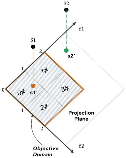
Figure 1.
Projection plane, projection grid, projection point, and objective domain.
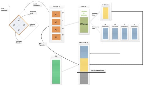
Figure 2.
MOEA/PII working process.
Assuming a 4-objective problem, where f1, f2, f3, and f4 are the objectives, users have selected f1 and f2 as the projection plane, and determined the objective domain according to their requirements, i.e., the values of f1 and f2 are both within the range of [0, 2]. Each projection dimension is divided into two segments, resulting in four projection cells, as shown in Figure 1. The free dimension algorithm employs MOEA/DD. The population N is initialized in each projection grid, with individuals saved in the SourceList. After performing crossover and mutation operations, the generated offspring are saved in the GenList.
Assuming S1 and S2 are two individuals in the GenList, after calculating the objective values for each dimension, we obtain S1 (0.8, 0.8, 3,4), S2 (2.5, 0.5, 2,6). s1′ (0.8, 0.8) and s2′ (2.5, 0.5) are the projection points of S1 and S2 on the projection plane, respectively. s1′ (0.8, 0.8) falls into the projection grid G0 and is saved in the ConEliteList(0); s2′ (2.5, 0.5) falls outside the determined objective domain and is saved in the ProEliteList. When the individuals are saved into the corresponding elite list, the free dimension algorithm is used to perform dominance sorting.
After completing the evolution of all individuals in the GenList, the ConEliteList(i) (where i is from 0 to 3) and ProEliteList are formed. The ConEliteList(i) is sequentially put into a temporary solution set according to the dominance results. If it is not sufficient to reach the population size, individuals from the ProEliteList are supplemented until the population size is reached. The individuals in this temporary solution set are saved in the OSS and are used as the initial population for the next iteration evolution. The solution set generated in each iteration is stored in the OSS according to the dominance relationship.
The convergence of MOEA/PII is determined by the free dimension algorithm. The distribution is guaranteed by the uniform partition of the projection grid. By determining the objective domain, individuals that do not meet user requirements cannot participate in evolution, making evolution more effective. Applications in the real world, such as WSN deployment problems, are detailed in Section 4.
The MOEA/PII framework working process is expressed in the algorithm. The meanings of the notations used in the algorithm are shown in Table 2.
Table 2.
The meanings of notations in algorithms.
The Algorithms 1 and 2 works as follows:
| Algorithm 1: MOEA/PII |
| Input: (1) Many-Objective Problem (MaOP); (2) End condition; (3) DS: Objective decision space; (4) NumOfGrids: the number of projection grid; (5) E: Evolution generation; (6) N: Initial Population Size; (7) Free Dimension Algorithm; Output: Objective Solution Set (OSS); Algorithm:
}
|
| Algorithm 2: Bi-Elite |
| Input: (1) GenList (2) NumOfNeighbor: the number of Neighbor; (3) NeighborPool: the neighbor vector; (4) Free Dimension Algorithm; Output: Bi-Elite Queue of each projection grid: ConEliteList(i) and ProEliteList; Algorithm: For each p in GenList {
|
3.2. The Advantage of Bi-Elite Strategy
- N: population size
- M: the number of objectives
- Sorting //() times
- Apply the MOEA/PII algorithm framework with Bi-Elite strategy
- P: the number of the projection plane dimensions
- F: the number of free dimensions
- M = P + F
- If ConEliteList(S) ← In(ProjectionGrid, N)
- ProEliteList(R) ← Out(ObjectiveDomain, N)
- And N = S + R
- Then For each S in ConEliteList on F free dimensions
- Sorting //() times
- For each R in ProEliteList on P projection plane
- Sorting //()times
We can see that , so the Bi-Elite strategy compressed the evolutionary magnitude.
3.3. Computational Complexity Analysis
- 1.
- The complexity of the crossover and mutation operation.
For each generation, with the crossover probability of 1.0 and the mutation probability of 1.0 (1/n), we can obtain four individuals for each individual in the population. The size of the initial population is N, and the offspring population is . Each individual should be compared with the others in the population. The sorting complexity is .
- 2.
- The complexity of the Bi-Elite sorting.
We choose the binary search as the sorting approach to the Bi-Elite queues. The number of solutions in ConEliteList is , and the number of free dimension is . The complexity of sorting in the ConEliteList is . The number of solutions in the ProEliteList is , and the number of projection plane dimension is . The complexity of sorting in the ProEliteList is . The total complexity of sorting with the Bi-Elite strategy is , where M = F + P and N = S + R. Correspondingly, the complexity of binary search without a Bi-Elite strategy is .
We can see that the Bi-Elite strategy compressed the evolutionary magnitude,
4. Experimental Studies and Discussions
4.1. Benchmark Test Instances
In our experiments, each algorithm was ran independently 30 times for each test instance. We introduce the general parameter settings for the experiments. The benchmark test instances of DTLZ1-7. It is widely used in the comparison of multi-objective evolutionary algorithms. DTLZ [35] was designed by Deb, K., Thiele, L., Laumanns, M., and Zitzler in 2002. The DTLZ test instances have different characteristics, and this creates many difficulties for the algorithm to converge to the Pareto front. DTLZ1 and DTLZ3 include many difficulties for the algorithm to converge to the Pareto front. DTLZ2 and DTLZ4 are used to test the ability of the algorithm to deal with different shape problems. DTLZ3 is a highly multimodal problem. DTLZ4 is a test problem whose density of the points on the true PF is strongly biased. This test problem is designed to verify whether an MOEA is able to maintain a proper distribution of the candidate solutions. DTLZ5 and DTLZ6 are the degenerated test problems, whose PFs are irregular. The DTLZ7 test problem has disconnected and degenerate PFs.
In addition, the benchmark test instances of WFG1-9 [36] are widely used in the comparison of multi-objective evolutionary algorithms. WFG was proposed by Walking Fish Group. WFG1 is designed with a flat bias and a mixed structure of the PF. WFG2 is a test problem that has a disconnected PF. WFG3 is a difficult problem where the PF is degenerate and the decision variables are non-separable. WFG4 to WFG9 are designed with different difficulties in the decision space. WFG4 is a multi-modal problem, WFG5 is a landscape deception problem and WFG6, WFG7, WFG8, and WFG9 are non-separable; their true PFs are the same convex structure. All of them can be extended to any number of objectives and decision vectors.
4.2. Performance Indicator
- 1.
- IGD-metric.
Inverted generational distance (IGD) [37] was used as the performance metric in our experimental analysis. IGD measures the average distance from a set of solutions in the true PF to the approximation solution set S.
It can be formulated as follows in (2):
where is a solution set uniformly sampled in the true PF. dist(x, S) is the Euclidean distance between the solution S and its nearest point x ∈ , and || is the cardinality of . The smaller the value of IGD, the better its convergence and diversity, and the closer it is to the true PF. It indicates that S is the sub-set of when . can measure both the diversity and convergence of S in a sense.
- 2.
- HV-metric.
Hyper-volume (HV) [38] is the volume of the objective space dominated by the approximate solution set with the bounded of · is dominated by all the solutions in the approximation solution set , where is the reference point in the objective space.
It can be formulated as follows in (3):
where is the objective function value of . The larger the value of HV, the closer it is to the true PF. HV is affected by the number of objectives and the selection of reference points.
- 3.
- C-metric.
C-metric [39] is an indicator to evaluate the convergence performance of the algorithm using two PF approximate solution sets, and its calculation is based on the Pareto-dominance relationship. Suppose A and B comprise the approximate solution set, then the C-metric represents the proportion shown in (4), in which the individuals in B are dominated by at least one individual in A.
C-metric (A,B) = 1 means that all individuals in B are dominated by individuals in A, that is, the convergence of A is better.
4.3. Experiments on Pareto Front
In order to investigate the performance of algorithms with MOEA/PII framework, the experiments were carried out on the benchmark test cases. Throughout this paper, we use an abbreviation of N3P2 to denote the algorithm NSGAIII with the MOEA/PII framework, and DDP2 to denote the algorithm MOEA/DD with the MOEA/PII framework.
In addition, all of the algorithms compared in this study have several parameters. The parameters of the crossover operator and mutation operator are shown in Table 3.
Table 3.
Parameter settings.
In an effort to compare the performance of algorithms, we set the population size and generations for the original algorithms (1000, 1000). When applying the MOEA/PII framework, the population initializes in each projection grid, so the number of initial population size will increase by a certain multiple. The population size is calculated by the number of projection grids (G), 1000⁄G. Accordingly, the generation size for the algorithms with MOEA/PII is calculated by the number of projection dimensions (D), 1000/(D + 1). For example, if the number of the projection dimension is 3 and there are 2 segments on each dimension, the generation size is 250 and population size is 125. The parameters of generations and population size are shown in Table 4.
Table 4.
General parameter settings. Number of generations for different algorithms (generations and population size).
DTLZ1 includes many difficulties, so it is a challenge for the algorithm to converge to the Pareto front. DTLZ4 has different shape problems, so that the density of the points on the true PF is strongly biased. DTLZ5 is a degenerated test problem whose PFs are irregular. WFG1, WFG2, and WFG3 are a mixed structure, disconnected, and degenerate, respectively. They have a certain degree of representativeness.
It is worth noting that for the benchmark problem DTLZ and WFG, DDP2 and N3P2 tend to obtain more diverse Pareto approximate solutions in the PF with 3-objective, as illustrated in Figure 3 and Figure 4.
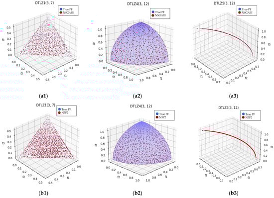
Figure 3.
Plot of the approximate PFs with NSGAIII and N3P2 for benchmark test instance DTLZ1, DTLZ4, and DTLZ5 with 3-objective. From (a1–a3) with NSGAIII, and from (b1–b3) with N3P2.
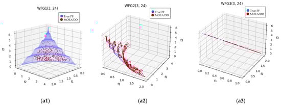
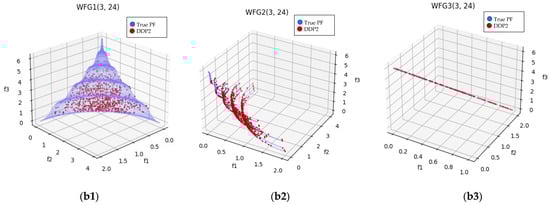
Figure 4.
Plot of the approximate PFs with MOEA/DD and DDP2 for benchmark test instance WFG1-3 with 3-objective. From (a1–a3) for WFG1-3 with MOEA/DD, from (b1–b3) with DDP2.
In order to observe the performance of DDP2 and N3P2 on MaOPs visually, the parallel coordinates of the non-dominated front obtained by the MOEA/DD and DDP2 algorithms on DTLZ1-4 DTLZ1, DTLZ4, and DTLZ5 with 15-objective, and those obtained by the NSGAIII and N3P2 algorithms on WFG1-4 with 10-objective are depicted in Figure 5 and Figure 6, respectively. As can be seen, DDP2 and N3P2 were able to obtain a solution set with a better diversity.
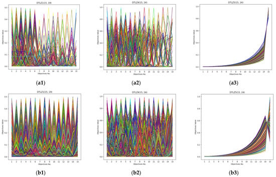
Figure 5.
Parallel coordinates of the non-dominated solutions obtained by MOEA/DD and DDP2 for benchmark test instances DTLZ1, DTLZ4, and DTLZ5 with 15-objective. From (a1–a3) with MOEA/DD, and from (b1–b3) with DDP2 (legends: each colored line represents a solution).
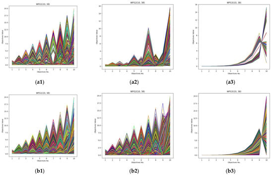
Figure 6.
Parallel coordinates of the non-dominated solutions obtained by NSGAIII and N3P2 for benchmark test instance WFG1-3 with 10-objective. From (a1–a3) with NSGAIII, and from (b1–b3) with N3P2 (legends: each colored line represents a solution).
4.4. Perfomance Analysisc
The results of the IGD-metric values obtained by the MOEA/DD and DDP2 algorithms on the DTLZ test instances are summarized in Table 5, in which the best results are highlighted. The results of the IGD-metric values obtained by the NSGAIII and N3P2 algorithms on the WFG test instances are summarized in Table 6, in which the best results are highlighted. The results of the HV-metric values obtained by the NSGAIII and N3P2 algorithms on the DTLZ test instances are summarized in Table 7, in which the best results are highlighted.
Table 5.
The mean and deviation value of the IGD-metric of MOEA/DD and DDP2 from 30 independent runs for each DTLZ test instance. Best performance is highlighted in bold face in gray background.
Table 6.
The mean and deviation value of the IGD-metric of NSGAIII and N3P2 from 30 independent runs for each WFG test instance. Best performance is highlighted in bold face in gray background.
Table 7.
The mean and deviation value of the HV-metric of NSGAIII and N3P2 from 30 independent runs for each DTLZ test instance. Best performance is highlighted in bold face in gray background.
In order to provide a visual representation, Figure 7a–c show the statistical trend in the data from Table 5, Table 6 and Table 7 respectively. Two groups of data from each table were chosen for a clear and intuitive illustration.
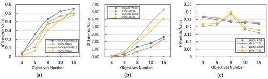
It can be seen that the algorithms (MOEA/DD and NSGAIII) with MOEA/PII framework exhibited the best performance on the benchmark test instances DTLZ1-7 and WFG1-9, with 3-, 5-, 8- 10-, and 15-objective.
4.5. Experiments on Projection Grids
This experiment was focused on projection grids with the MOEA/PII framework. After choosing the projection dimensions, we set the segments on them to carve the projection plane. Each projection dimension was segmented, and all segments of each dimension were combined to form the projection grids of the projection plane.
We ran the algorithms on the 5-objective DTLZ1 test instance and recorded the results of the IGD-metric values in Table 8 and Table 9.
Table 8.
The mean and deviation value of the IGD-metric of MOEA/DD and NSGAIII for 30 independent runs on 5-objective DTLZ1 test instance.
Table 9.
The mean and deviation value of the IGD-metric of DDP2 and N3P2 for 30 independent runs on 5-objective DTLZ1 test instance with different numbers of projection grids.
The column of projection grids in Table 9 and the X-axis coordinate scale in Figure 8 are annotated by the number of projection dimensions, segments per dimension, and projection grids. For example, a projection plane is two dimensional (2D), and each dimension is divided into two segments (2S/D). The number of combination is four, which is the number of projection grids (4G). It is recorded as 2D_2S/D_4G.
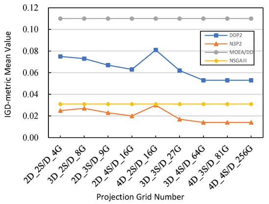
Figure 8.
The mean value of the IGD-metric obtained by MOEA/DD, NSGAIII, DDP2, and N3P2 on the 5-objective DTLZ1 benchmark test instance with different numbers of projection grids.
Figure 8 shows the mean value of the IGD-metric obtained by MOEA/DD, NSGAIII, DDP2, and N3P2 on the 5-objective DTLZ1 benchmark test instance with different numbers of projection grids. We can see that for the same number of projection dimensions, the more segments there are, the more the projection grids, and the better the IGD-metric value.
There was also another scenario of 2D_4S/D_16G and 4D_2S/D_16G, which was different. We know that the IGD-metric value expresses the convergence and diversity of the algorithm at the same time. Because 4D_2S/D_16G has two segments for each dimension, the diversity is worse than for four segments for each dimension (2D_4S/D_16G). Therefore, the IGD-metric value of 2D_4S/D_16G was better than that of 4D_2S/D_16G. In addition, for the same number of projection grids, we should choose the fewest projection dimensions and more segments.
4.6. Experiments on Wireless Sensor Networks (WSNs) Deployment Problem
Since the performance of the proposed algorithm was competitive on unconstrained test problems, we investigated its performance on wireless sensor networks deployment problem [40]. When we deploy sensor nodes, we need to consider a series of problems, such as the coverage of the detection space, the connectivity among sensor nodes, the cost, the network life cycle, and so on. However, there are mutual constraints and imbalanced goals among these problems, so we usually regard them as multi-objective optimization problems.
Suppose that a 100-square-meter plane with a width of 10 m and a length of 10 m is evenly divided into grids, each denoted Cij. This is the detection area detected by the WSN composed of a set of sensor nodes.
The WSN is composed of a set of sensors and a set of sink nodes . The cost of the wireless sensor network includes two parts: the sensor node cost and sink node cost. The cost can be calculated using (5).
where Cs and Csk represent the purchase costs of the sensor node and sink node, respectively. are the quantity of sets S and SK, respectively.
Each sensor node has a sensing area and can sense a target within its sensing radius R. The Euclidean distance between Cij and the sensor node Si is denoted d(Cij, Si). The case in which the target Cij is covered is represented by (6).
The coverage fraction can be calculated by (7).
Information transmission in WSNs should ensure security, efficiency, and reliability, and connectivity can be evaluated based on the received signal strength calculated at the receiving node. In the process of radio propagation, assuming the signal transmission point is bij, the signal strength at this point is PTX, and the receiving point is nij. The received signal strength at this point is RSSI(i, j). The relationship between the transmitted signal strength and the received signal strength is expressed in (8).
The connection is calculated by the , which is greater than the minimum signal strength Ptsh required for communication or not. This is shown in (9).
The connectivity fraction can be calculated using (10).
The deployment cost is relative to the number of sensor nodes; the coverage fraction satisfies the maximum coverage of the detection area and the connectivity. are the objectives to be optimized. We want to obtain the highest coverage and connectivity for the lowest cost (with the fewest sensor nodes). These objectives are in conflict, which makes finding the optimal solution difficult, creating a multi-objective problem.
4.6.1. Compare the C-Metric between Algorithms and with the MOEA/PII Framework
We compare the coverage performance of the MOEA/DD algorithm and DDP2 algorithm, and NSGAIII algorithm and N3P2 algorithm using the C-metric indicator. The results are shown in Table 10 and Table 11, with a generation iteration of 500. We can see in Table 10 that 23.2% of the solutions in the solution set obtained by MOEA/DD were dominated by those obtained by DDP2. Instead, only 1.5% of the solutions in the solution set obtained by DDP2 were dominated by MOEA/DD. This means that the solutions in the solution set obtained by DDP2 were better than those obtained by the MOEA/DD algorithm. In addition, in Table 11, we can see that 18.8% of the solutions in the solution set obtained by NSGAIII were dominated by those obtained by N3P2. Instead, only 10.6% of the solutions in the solution set obtained by N3P2 were dominated by NSGAIII. This indicates that the solutions in the solution set obtained by N3P2 were better than those obtained by the NSGAIII algorithm.
Table 10.
The comparison of C-Metric between MOEA/DD and DDP2.
Table 11.
The comparison of C-Metric between NSGAIII and N3P2.
4.6.2. Experiments on Determining the Objective Domain
The optimal WSN deployment solution uses the fewest sensor nodes to obtain the highest connectivity and coverage fraction. This is a multi-objective optimization problem. Multi-objective optimization evolutionary algorithms can solve these. However, the algorithms obtain a set of non-dominated solutions, and some of them are not suitable for customers. This makes it difficult for the customer to choose a suitable solution. If they prefer a high coverage fraction, they further filter the solutions.
We chose the N3P2 algorithm, set the population size to 60 and the generation iteration to 100, and ran the experiment 30 times independently to obtain the average value for comparison.
In the same deployment scenario, we set the cost and connectivity () as the free dimensions, and the coverage fraction () as the projection plane. In one experiment, there was no determination on any dimensions. In the other experiment, the objective domain on the projection plane of the coverage fraction () was determined, and the objective domain was from 50% to 100%.
We can see in Table 12 that when no dimensions were determined, the algorithm ran for a long time but obtained less satisfactory solutions than what was required by the customer. Determining the objective domain of the objects of the wireless sensor networks deployment problem made the solution set run faster and made it more responsive to user needs.
Table 12.
The comparison of the average time and number of solutions that meet user requirements by determining the objective domain or not with N3P2 algorithm.
5. Conclusions
This paper proposes a MOEA/PII algorithm framework to solve many-objective optimization problems. MOEA/PII is an algorithm framework based on projection plane. Different from the other MOEAs for MaOPs, the MOEA/PII is a framework that can be combined with the original algorithms. Some objective dimensions are chosen to be the projection plane, which evolve via the projection grids. The left objective dimensions are the free dimensions that evolve via the originally selected algorithm. In addition, the non-dominated solutions are sorted and temporarily stored in the convergence elite and projection elite lists. The population of the next generation is composed of the solutions in ConEliteLists, and the solutions in ProEliteList are added when the population quantity is not sufficient.
In an attempt to alleviate the problem of selection pressure, the MOEA/PII carves the projection plane into projection grids, and the evolution process is carried out in each grid. In each projection grid, the number of individuals to be selected decreases, and accordingly, the selection pressure is alleviated.
The mechanism of Bi-Elite ensures that there are solutions in each grid. In the MOEA/PII framework, the distribution of the projection grid is uniform, which ensures the overall distribution of the solutions. The convergence of the solutions in each grid is determined by the free dimension algorithm.
In addition, we assessed the performance of the MOEA/PII framework from five aspects. First, the solutions set produced by MOEA/PII on 3-objective test instances was closer to Pareto fronts and was well-distributed on the PFs. For 15-objective test instances, the solutions were shown in the parallel coordinate. Secondly, we compared the IGD-metric and HV-metric values of the original algorithms and the original algorithms with the MOEA/PII framework running on benchmark test instances, i.e., DTLZ1-7 and WFG1-9, with 3, 5, 8, 10, and 15 objectives. The findings of this study support the idea that the MOEA/PII framework is efficient. Thirdly, the experiments demonstrated ways in which a projection grid could be chosen. The evidence from this study suggests that more segments lead to more projection grids, which improves the IGD-metric value. There was one exception: when we chose the fewest projection dimensions with more segments at the same number of grids. Fourthly, we investigated our framework’s performance on the wireless sensor networks deployment problem. The solutions in the solution set obtained by the algorithms with MOEA/PII were better than those obtained by the original algorithms. Finally, when the user determined the objective domain, the solution set was more responsive to user needs, and the time was reduced.
The experiments were carried on two state-of-the-art MOEAs (MOEA/DD and NSGAIII) on DTLZ1-7, WFG1-9 benchmark test instances, and a wireless sensor networks deployment problem, which demonstrated superior performance with MOEA/PII. In summary, these findings highlight a role for the MOEA/PII framework. Our study provides a novel framework for solving MaOPs.
Author Contributions
Conceptualization, F.P., L.L. and W.C.; methodology, F.P. and W.C.; software, F.P. and W.C.; validation, L.L. and J.W.; investigation, L.L. and J.W.; writing—original draft preparation, F.P.; writing—review and editing, F.P. All authors have read and agreed to the published version of the manuscript.
Funding
This research was supported by the Regional Key Project of the Science and Technology Service Network Plan (STS Plan) of the Chinese Academy of Sciences (Grant No. KFJ-STS-QYZD-2021-19-003).
Data Availability Statement
The data presented in this study are available on request from the corresponding author. The data are not publicly available due to privacy.
Acknowledgments
The authors sincerely appreciate the support from the Scientific research project of Liaoning Province Education Department (LJKMZ20220783) and (LJKMZ20220781); the national foreign expert project plan (G2022006008L); China University Innovation Fund (2021LD06009); the Liaoning Province’s “million talents project” (LRS [2019] No. 45); the Liaoning Province Nature Fund Project (No. 2022-MS-291); the Scientific research project of Liaoning Province Department of Education (LJ2020024, 2022); the Basic Research Project of Education Department of Liaoning Province (No. LJ2020022); the Opening Project of Beijing Key Laboratory of Sensors of Beijing Information Science and Technology University (2020CGKF005).
Conflicts of Interest
The authors declare no conflict of interest.
References
- Zhou, A.M.; Qu, B.Y.; Li, H.; Zhao, S.Z.; Suganthan, P.N.; Zhang, Q.F. Multiobjective evolutionary algorithms: A survey of the state of the art. Swarm Evol. Comput. 2011, 1, 32–49. [Google Scholar] [CrossRef]
- Behmanesh, R.; Rahimi, I.; Gandomi, A.H. Evolutionary Many-Objective Algorithms for Combinatorial Optimization Problems: A Comparative Study. Arch. Comput. Methods Eng. 2021, 28, 673–688. [Google Scholar] [CrossRef]
- Pereira, J.L.J.; Oliver, G.A.; Francisco, M.B.; Cunha, S.S.; Gomes, G.F. A Review of Multi-objective Optimization: Methods and Algorithms in Mechanical Engineering Problems. Arch. Comput. Methods Eng. 2022, 29, 2285–2308. [Google Scholar] [CrossRef]
- Osamy, W.; Khedr, A.M.; Salim, A.; Al Ali, A.I.; El-Sawy, A.A. Coverage, Deployment and Localization Challenges in Wireless Sensor Networks Based on Artificial Intelligence Techniques: A Review. IEEE Access 2022, 10, 30232–30257. [Google Scholar] [CrossRef]
- Benatia, M.A.; Sahnoun, M.; Baudry, D.; Louis, A.; El-Hami, A.; Mazari, B. Multi-Objective WSN Deployment Using Genetic Algorithms Under Cost, Coverage, and Connectivity Constraints. Wirel. Pers. Commun. 2017, 94, 2739–2768. [Google Scholar] [CrossRef]
- Bi, W.W.; Chen, M.J.; Shen, S.W.; Huang, Z.Y.; Chen, J. A Many-Objective Analysis Framework for Large Real-World Water Distribution System Design Problems. Water 2022, 14, 13. [Google Scholar] [CrossRef]
- Liu, J.; Huang, J.; Hu, J.Z. Multi-objective optimisation method of electric vehicle charging station based on non-dominated sorting genetic algorithm. Int. J. Glob. Energy Issue 2022, 44, 413–426. [Google Scholar] [CrossRef]
- Barakat, N.; Sharma, D. Evolutionary multi-objective optimization for bulldozer and its blade in soil cutting. Int. J. Manag. Sci. Eng. Manag. 2019, 14, 102–112. [Google Scholar] [CrossRef]
- Colombo, L.; Todd, M.D.; Sbarufatti, C.; Giglio, M. On statistical Multi-Objective optimization of sensor networks and optimal detector derivation for structural health monitoring. Mech. Syst. Signal Process. 2022, 167, 20. [Google Scholar] [CrossRef]
- Otis, M.J.D.; Vandewynckel, J. A Many-Objective Simultaneous Feature Selection and Discretization for LCS-Based Gesture Recognition. Appl. Sci. 2021, 11, 9787. [Google Scholar] [CrossRef]
- Petchrompo, S.; Coit, D.W.; Brintrup, A.; Wannakrairot, A.; Parlikad, A.K. A review of Pareto pruning methods for multi-objective optimization. Comput. Ind. Eng. 2022, 167, 22. [Google Scholar] [CrossRef]
- He, Z.A.; Yen, G.G. Many-Objective Evolutionary Algorithm: Objective Space Reduction and Diversity Improvement. IEEE Trans. Evol. Comput. 2016, 20, 145–160. [Google Scholar] [CrossRef]
- Zhu, C.W.; Xu, L.H.; Goodman, E.D. Generalization of Pareto-Optimality for Many-Objective Evolutionary Optimization. IEEE Trans. Evol. Comput. 2016, 20, 299–315. [Google Scholar] [CrossRef]
- Yang, S.X.; Li, M.Q.; Liu, X.H.; Zheng, J.H. A Grid-Based Evolutionary Algorithm for Many-Objective Optimization. IEEE Trans. Evol. Comput. 2013, 17, 721–736. [Google Scholar] [CrossRef]
- Karimi, N.; Feylizadeh, M.R.; Govindan, K.; Bagherpour, M. Fuzzy multi-objective programming: A systematic literature review. Expert Syst. Appl. 2022, 196, 19. [Google Scholar] [CrossRef]
- He, Z.N.; Yen, G.G.; Zhang, J. Fuzzy-Based Pareto Optimality for Many-Objective Evolutionary Algorithms. IEEE Trans. Evol. Comput. 2014, 18, 269–285. [Google Scholar] [CrossRef]
- Menchaca-Mendez, A.; Montero, E.; Antonio, L.M.; Zapotecas-Martinez, S.; Coello, C.A.; Riff, M.C. A Co-Evolutionary Scheme for Multi-Objective Evolutionary Algorithms Based on epsilon-Dominance. IEEE Access 2019, 7, 18267–18283. [Google Scholar] [CrossRef]
- Wu, T.W.; An, S.G.; Han, J.Q.; Shentu, N.Y. An epsilon-domination based two-archive 2 algorithm for many-objective optimization. J. Syst. Eng. Electron. 2022, 33, 156–169. [Google Scholar] [CrossRef]
- Yuan, Y.; Xu, H.; Wang, B.; Yao, X. A New Dominance Relation-Based Evolutionary Algorithm for Many-Objective Optimization. IEEE Trans. Evol. Comput. 2016, 20, 16–37. [Google Scholar] [CrossRef]
- Zhang, Q.; Hui, L. MOEA/D: A Multiobjective Evolutionary Algorithm Based on Decomposition. IEEE Trans. Evol. Comput. 2008, 11, 712–731. [Google Scholar] [CrossRef]
- Sun, Y.H.; Xiao, K.L.; Wang, S.Q.; Lv, Q.Y. An evolutionary many-objective algorithm based on decomposition and hierarchical clustering selection. Appl. Intell. 2022, 52, 8464–8509. [Google Scholar] [CrossRef]
- Zhao, H.T.; Zhang, C.S.; Zhang, B.; Duan, P.B.; Yang, Y. Decomposition-based sub-problem optimal solution updating direction-guided evolutionary many-objective algorithm. Inf. Sci. 2018, 448, 91–111. [Google Scholar] [CrossRef]
- Asafuddoula, M.; Ray, T.; Sarker, R. A Decomposition-Based Evolutionary Algorithm for Many Objective Optimization. IEEE Trans. Evol. Comput. 2015, 19, 445–460. [Google Scholar] [CrossRef]
- Sun, Y.A.; Yen, G.G.; Yi, Z. IGD Indicator-Based Evolutionary Algorithm for Many-Objective Optimization Problems. IEEE Trans. Evol. Comput. 2019, 23, 173–187. [Google Scholar] [CrossRef]
- Liu, C.; Zhao, Q.; Yan, B.; Gao, Y. A new hypervolume-based differential evolution algorithm for many-objective optimization. Rairo-Oper. Res. 2017, 51, 1301–1315. [Google Scholar] [CrossRef]
- Shang, K.; Ishibuchi, H.; He, L.J.; Pang, L.M. A Survey on the Hypervolume Indicator in Evolutionary Multiobjective Optimization. IEEE Trans. Evol. Comput. 2021, 25, 1–20. [Google Scholar] [CrossRef]
- Li, F.; Cheng, R.; Liu, J.C.; Jin, Y.C. A two-stage R2 indicator based evolutionary algorithm for many-objective optimization. Appl. Soft. Comput. 2018, 67, 245–260. [Google Scholar] [CrossRef]
- Dhiman, G.; Soni, M.; Pandey, H.M.; Slowik, A.; Kaur, H. A novel hybrid hypervolume indicator and reference vector adaptation strategies based evolutionary algorithm for many-objective optimization. Eng. Comput. 2021, 37, 3017–3035. [Google Scholar] [CrossRef]
- de Oliveira, M.C.; Delgado, M.R.; Britto, A. A hybrid greedy indicator- and Pareto-based many-objective evolutionary algorithm. Appl. Intell. 2021, 51, 4330–4352. [Google Scholar] [CrossRef]
- Dhiman, G.; Kumar, V. KnRVEA: A hybrid evolutionary algorithm based on knee points and reference vector adaptation strategies for many-objective optimization. Appl. Intell. 2019, 49, 2434–2460. [Google Scholar] [CrossRef]
- Xiang, Y.; Zhou, Y.R.; Tang, L.P.; Chen, Z.F. A Decomposition-Based Many-Objective Artificial Bee Colony Algorithm. IEEE Trans. Cybern. 2019, 49, 287–300. [Google Scholar] [CrossRef] [PubMed]
- Zhao, H.T.; Zhang, C.S.; Zhang, B. A decomposition-based many-objective ant colony optimization algorithm with adaptive reference points. Inf. Sci. 2020, 540, 435–448. [Google Scholar] [CrossRef]
- Qiu, W.B.; Zhu, J.H.; Wu, G.H.; Fan, M.F.; Suganthan, P.N. Evolutionary many-Objective algorithm based on fractional dominance relation and improved objective space decomposition strategy. Swarm Evol. Comput. 2021, 60, 16. [Google Scholar] [CrossRef]
- Lu, X.; Yang, S.; Peng, F.; Chen, W. An Evolutionary Algorithm for Multi-objective Optimization Problem Based on Projection Plane: MOEA/P. In Proceedings of the 2021 The 5th International Conference on Algorithms, Computing and Systems, Xi’an, China, 24–26 September 2021. [Google Scholar]
- Deb, K.; Thiele, L.; Laumanns, M.; Zitzler, E. Scalable multi-objective optimization test problems. In Proceedings of the Congress on Evolutionary Computation, Honolulu, HI, USA, 12–17 May 2002. [Google Scholar]
- Huband, S.; Hingston, P.; Barone, L.; While, L. A review of multiobjective test problems and a scalable test problem toolkit. IEEE Trans. Evol. Comput. 2006, 10, 477–506. [Google Scholar] [CrossRef]
- Zhang, Q.; Zhou, A.; Zhao, S.; Suganthan, P.N.; Tiwari, S. Multiobjective optimization Test Instances for the CEC 2009 Special Session and Competition. Mech. Eng. 2008, 1–29. Available online: https://www.researchgate.net/publication/265432807_Multiobjective_optimization_Test_Instances_for_the_CEC_2009_Special_Session_and_Competition (accessed on 17 April 2023).
- Zitzler, E.; Thiele, L.; Laumanns, M.; Fonseca, C.M.; Fonseca, V. Performance assessment of multiobjective optimizers: An analysis and review. IEEE Trans. Evol. Comput. 2003, 7, 117–132. [Google Scholar] [CrossRef]
- Zitzler, E.; Thiele, L. Multiobjective evolutionary algorithms: A comparative case study and the strength Pareto approach. IEEE Trans. Evol. Comput. 1999, 3, 257–271. [Google Scholar] [CrossRef]
- Lv, L.; Peng, F.; Chen, W.; Wang, J. Node Deployment of Wireless Sensor Networks Based on MOEA/P Algorithm. In Proceedings of the 2021 13th International Conference on Communication Software and Networks (ICCSN), Chongqing, China, 4–7 June 2021. [Google Scholar]


Disclaimer/Publisher’s Note: The statements, opinions and data contained in all publications are solely those of the individual author(s) and contributor(s) and not of MDPI and/or the editor(s). MDPI and/or the editor(s) disclaim responsibility for any injury to people or property resulting from any ideas, methods, instructions or products referred to in the content. |
© 2023 by the authors. Licensee MDPI, Basel, Switzerland. This article is an open access article distributed under the terms and conditions of the Creative Commons Attribution (CC BY) license (https://creativecommons.org/licenses/by/4.0/).