Article

Mixing Transport Mechanism of Three-Phase Particle Flow Based on CFD-DEM Coupling

1
Special Equipment Institute, Hangzhou Vocational and Technical College, Hangzhou 310018, China
2
College of Mechanical and Automotive Engineering, Zhejiang University of Water Resources and Electric Power, Hangzhou 310018, China
*
Author to whom correspondence should be addressed.
Processes 2023, 11(6), 1619; https://doi.org/10.3390/pr11061619
Submission received: 30 April 2023 / Revised: 15 May 2023 / Accepted: 23 May 2023 / Published: 25 May 2023

Abstract

:
The mixing transport courses of three-phase particle flows exist in some industrial applications, such as metallurgy material extraction, lithium electric slurry dispersion, and material mixing in the high-end chemical industry. Its mixing transport mechanism is a fluid–structure coupling dynamic issues with intensive shear and nonlinear characteristics, making the real-time prediction of the flow field face challenges. To address the above problem, a bidirectional fluid–structure coupling three-phase particle flow dynamic model is built based on the coupled computational fluid dynamics and discrete element model (CFD-DEM) to explore the mixing transport mechanism. An interphase coupling solution method is utilized to solve the interaction effects of the fluid and particle. Research results illustrate that the proposed method modeling can well reveal the mixing transport mechanism of the three-phase particle flows. Due to the additive effects of stirring speed, stirring blade size, and stirring blade structure, the flow field near the blade has a high-velocity gradient change, while the flow field away from the stirring blade has no significant change. When the particle material settles and accumulates to a certain extent, the particle movement is blocked, and the stirring speed of the particle material near the blade is reduced. The mixing effect of the particle material will be reduced near the wall. It can provide a valuable reference for particle flow transport and pattern identification and support technical support for lithium electric homogenate mixing, chemical extraction, and pharmacy process regulation.

1. Introduction

With the rapid development of modern industry, material mixing is an essential part of industrial production, which is often used to disperse two or more different substances in the industrial scene so that the material phase distribution is more uniform [1,2,3]. The mixing process involves the chemical and physical changes of mixed materials, among which the most common application scene is mixing. Take the production of lithium batteries standard in the new energy industry; in the positive and negative slurry, the dispersion and uniformity of granular active substances directly affect the movement of lithium ions between the two poles of the battery. In lithium-ion battery production, the slurry mixing and dispersion effect of bipolar sheet material is critical. The quality of slurry dispersion directly affects the production quality of lithium batteries and their performance [4,5,6,7]. Therefore, it has significant scientific research value and engineering application prospects to study the mixed transport process of gas–liquid–solid three-phase flow and analyze the material transport and flow pattern evolution process.
In practical engineering mixing systems, gas and liquid are usually regarded as continuous phases, while solid is regarded as dispersed phases. By selecting appropriate mixing execution components and physical space of flow channels, the goal of providing better interphase contact, mass transfer, and high turbulence ability can be achieved to accelerate mixing speed and realize uniform dispersion and complete mixing between different phases. In the physical space of the mixed runner, the impeller of the actuator transmits the generated energy to the nearby fluid through rotation, generating a violent three-dimensional flow, thus promoting the multiphase flow in the mixed space so that the materials can be dispersed and mixed better [8,9,10]. The flow mode of the flow field affects the quality of the product. However, the geometric scale of physical space is often many orders of magnitude higher than that of particles. The unpredictability of circulating flow makes the mixing process face great difficulties.
Related scholars have conducted a series of studies to solve the above problems. Xu studied the influence of the eddy current on the dispersion of mixed particles and found that the composite choke component could effectively control the eddy current and improve the uniformity of particle distribution [11]. Bao discussed the effect of impeller diameter on gas dispersion in mixed space and found that gas holdup simulation at lower gas velocities was consistent with experimental results [12]. Gu analyzed the hydrodynamic characteristics of the solid–liquid suspension process and found that the uniformity of the system increased with the increase in impeller speed [13]. Blais established a semi-analytical model to study the mixing dynamics of viscous suspensions and obtained the flow pattern and particle distribution [14]. Kou performed a numerical simulation study on the mixing characteristics of multiphase flow in an autoclave and found that the solid–liquid mixing is mainly affected by the axial flow [15]. At present, the research on multiphase flow mainly focuses on the liquid–solid phase and gas–liquid phase. The research on the mixing process of gas, liquid, and solid three-phase flow is limited. There is a lack of research and report on the mixed transport process of the flow field of complex executive components.
This paper proposes a CFD-DEM coupled modeling and solution method to study the gas–liquid–solid three-phase flow mixing process with complex executive components, and the dynamic evolution process of the three-phase flow field and the law of particle flow pattern are analyzed. The related research work provides a theoretical reference for the research of the multiphase mixing process. Additionally, it has essential technical value for chemical engineering, biopharmaceutical engineering, lithium electrosurgery dispersion, and other critical industrial fields.

2. Mathematical Model and Solution Method

2.1. Flow Field Control Equations

For the CFD method, the continuous fluid domain is discretized into grid cells [16,17]. In each grid cell, fluid velocity, pressure, and density are locally averaged quantities. The continuity and locally averaged Navier–Stokes equations for each grid cell are assumed as follows:
t ( α ρ ) + ( α ρ u f ) = 0 ,
t ρ u f + ( ρ u f u f ) = α p + α μ u f + α ρ g + S ,
where α is the porosity (void fraction), g is the gravitational acceleration, ρ is the averaged fluid density, p is the fluid pressure in the grid cell, uf is the average velocity of a fluid grid cell, μ is the averaged viscosity, and S is the interaction force.
The flow field can form the complete turbulence state under the initial velocity. The turbulence model should be considered in fluid control equations. As a classical turbulence model, the realizable k-ε model has been used in some industrial fields with its reliable robustness [18,19]. Moreover, it has a better computation performance on the flow fields with intensive streamlined curvature, vortex, and rotation. Thus, the realizable k-ε model is adopted to describe the turbulent motion of gas–liquid–solid mixing flows as follows:
ρ k t + ρ k u f x i = x j μ + μ t σ k k x j + G k ρ ε ,
ρ ε t + ρ ε u f x i = x j μ + μ t σ ε ε x j + ρ C 1 E ε ρ C 2 ε 2 k + ν ε ,
where E represents the modulus of time-averaged strain rate tensor, Gk is the turbulent kinetic energy caused by the average velocity gradient, σk and σε are the Prandtl number of turbulent kinetic energy k and dissipation rate ε, respectively, μt is the turbulent viscosity coefficient, and v is the kinematic viscosity.
In the realizable k-ε model, the turbulent viscosity coefficient μt is the critical parameter for turbulence computation and can be described as follows:
μ t = ρ C μ k 2 ε ,
C μ = 1 A 0 + A s U * k / ε ,
where Cμ is regarded as a variable, and A0 and As are the characteristic constants, which are expressed as follows:
A 0 = 4.04 A s = 6 cos φ .
According to Equations (5)–(7), it can be found that Cμ is a key variable of μt. It can be regarded as a function containing the parameters of rotation velocity, time-averaged strain, turbulent intensity, and angular velocity. Given the above features, the realizable k-ε model has the advantage of simulating the flow field of jet, boundary layer fluid, and rotation shear flow [20,21,22].

2.2. Discrete Element Method

DEM is a numerical analysis method for computing the structure and movement laws of non-continuous granular materials and analyzing the contact force and motion of discrete particles [23,24]. In this method, the motion of particles is modeled as a discrete phase, described by Newton’s laws of motion, on an individual scale. Therefore, the motion equations of a discrete particle in multiphase flow are expressed as follows:
m i = d u i d t = F a + F c + G ,
I i d ω i d t = T i ,
where Fc and G are the collision contact force and gravity of the particle, mi and ui are the mass and velocity of particle i, and Ii, ωi, and Ti are the rotary inertia, angular velocity, and torque of particle i, respectively. The formation of gas–liquid–solid mixing flow is an unsteady process, the forces of fluids acting on the particles are variable constantly, and the flow field has larger pressure and velocity gradient variation, so the forces acting on the particles mainly consider four aspects of drag force, pressure gradient force, Saffman lift force, and Magnus force. Consequently, the interaction force Fa between fluid and particle is described as follows:
F a = F d + F p + F s + F m ,
where Fd, Fp, Fs, and Fm represent drag force, pressure gradient force, Saffman lift force, and Magnus force, respectively. The drag force is a typical interphase force that plays a significant role in the forces acting on a particle. For the particle flow on the vortex center, there are high particle volume fractions. Therefore, the following drag force equation, which considers the effect of void fraction, is adopted [25,26,27]:
F d = 1 8 C d ρ π d p 2 u f u p u f u p α χ + 1 ,
where up and dp are the velocity and diameter of the particle, respectively. Cd is the particle-fluid drag coefficient, which depends on the Reynolds number of the particle Rep and is calculated via the following equation:
C d = 0.63 + 4.8 R e p 0.5 2 .
The particle Reynolds number is determined via
R e p = α ρ d p u f u p μ .
For the αχ in Equation (11), it denotes a corrective function to account for the effect of other particles on the drag force of the particle, wherein χ is expressed as follows [28,29,30,31]:
χ = 3.7 0.65 exp 1.5 log R e p 2 / 2 .
In addition, owing to the higher variations of velocity and pressure of the mixing flow field, the other three aspect forces of pressure gradient force, Saffman lift force, and Magnus force acting on the particles should be considered and can be calculated as follows:
F p = 1 6 π d p 3 d p d x ,
F s = 1.615 d p 2 ρ μ ( u f u p ) d u f d y ,
F m = π 8 d p 3 ρ ( ω × ( u p u f ) ) 1 + θ R ,
where θ(R) is a remainder, its order of magnitude is much smaller than other items. R is the remainder expansion point. Moreover, the selected particle has smaller volume and larger density features, and buoyant force and gravity need to be considered.
To acquire the contact effects for particle–particle and particle–wall, the soft sphere model is adopted to calculate the collision force. Particles i and j select springs and dampers to quantize the collision process. The collision force can be decomposed into a normal collision force and a tangential collision force and can be expressed as follows:
F n = ( k n a 3 2 η n G r n ) n ,
F t = k t δ η t G t ,
where Gt is the relative slip velocity in the contact point; Gr is the relative velocity between particle i and j; n is the unit vector from the sphere center of particle i to j; kn and ηn are the normal elastic coefficient and normal damping coefficient of particle i, respectively; kt and ηt are the tangential elastic coefficient and tangential damping coefficient.

2.3. An Interphase Coupling Solution Method for Fluid and Particle

In the coupled CFD-DEM scheme, the data interactions are conducted by calculating the interaction force (Fa) and porosity (α). In a grid cell, the sum of porosity (α) and the volume fraction (αp) equals one. Porosity can be obtained by calculating the volume fraction (αp). Firstly, the particles in a grid cell are surrounded by a bounding box, and then we count the sample points in the bounding box. If the sample points are located in the particle and grid cell, they will be saved, so the volume fraction of the particle in a grid cell can be obtained via
α p = 1 α = n c N v c ,
where nc is the sum of sample points in the particles and grid cell, and N is the sum of the sample points in a bounding box.

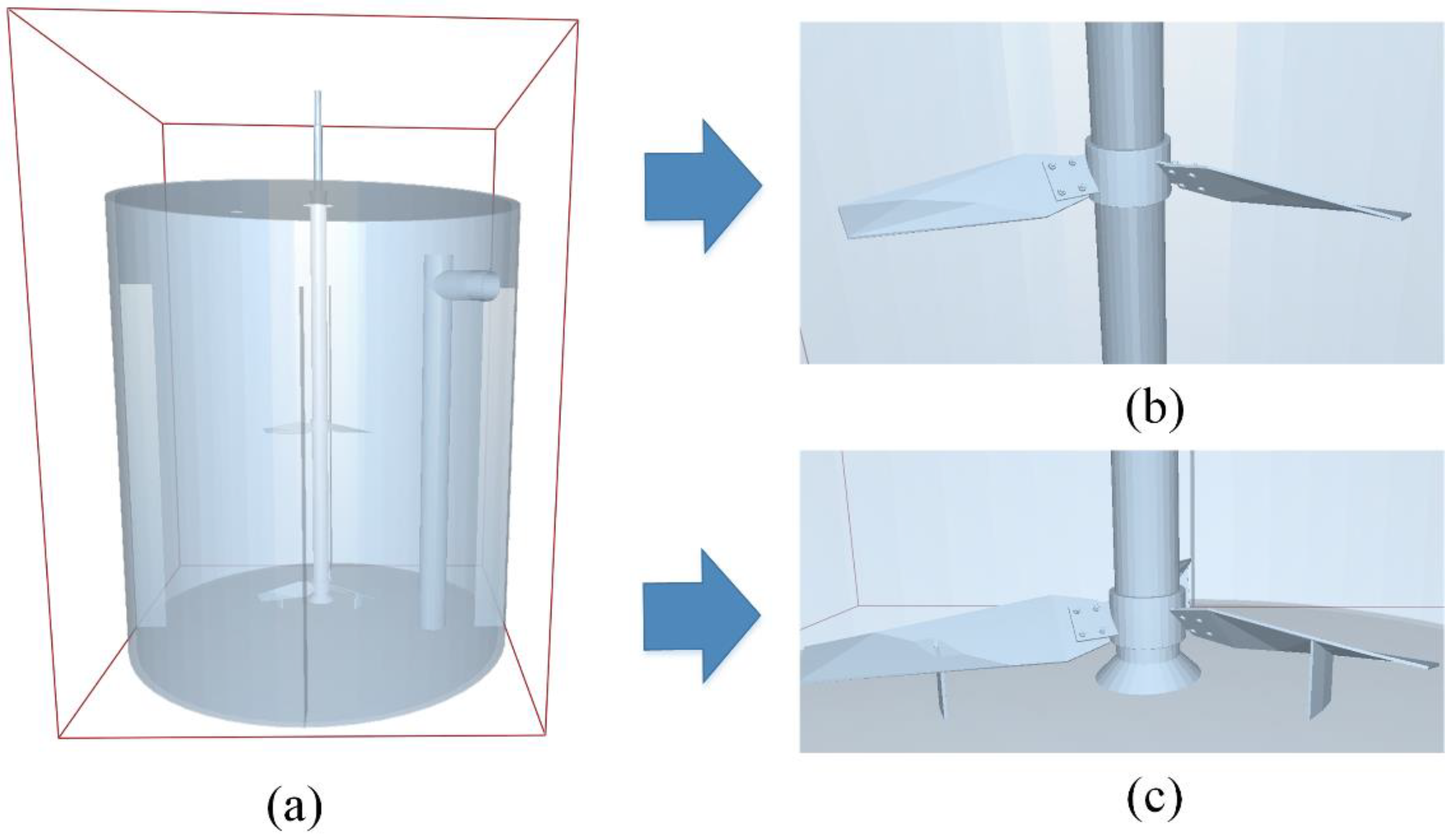
3. Model Implementation and Boundary Conditions

3.1. Physical and Numerical Models

Gas–liquid–solid multiphase flow is a typical flow state in physical space. In this case, the object of this article is a container with a baffle in a finite physical space (Figure 1). Because the three-dimensional structure near the blade is complex, the fine structure will not change the dynamic evolution law of the whole flow field in the engineering calculation. Therefore, according to the structure diagram of the mixing tank, the screws and nuts near the impeller and the tank structure are simplified. The physical model consists of a bottom air inlet, a baffle, and a double-layer impeller. The mixing actuator rotates under the initial driving conditions to mix the gas, liquid, and solid three-phase flows in the physical region. The gas is air, and the liquid is the mixture medium, including the cobaltous sulfate, caustic soda liquid, and ammonium hydroxide.
Due to the enormous size of the mixing tank, and the tiny size of the rotating blade and the whole inflating shaft, there is a large order of magnitude difference between the two, which is quite tricky for fine meshing. To solve the problem, the structure near the blade is extracted for fine mesh division because the blade surface of this part of the blade has a specific arc, and the structure is relatively complex. Therefore, the grid is divided into unstructured grids, with more than 1 million grids in blade parts, and the grid quality is guaranteed to be above 0.4. For the whole stirred tank, unstructured grids are used for division, whose mesh size is much larger than that near the blades, to improve the speed of numerical calculation. The overall grid division diagram is shown in Figure 2.

3.2. Boundary Conditions and Initial Conditions

In this model, the top of the mixing vessel is set as the pressure inlet boundary condition, the bottom of the center of the container is the inflatable tube, the velocity inlet boundary condition is adopted, and the container wall is the non-slip wall boundary condition. In the EDEM program, the soft sphere contact model is used to determine the phase plane and elasticity of the particles. The collision contact model based on the damping coefficient calculates the contact process between particles and the wall surface. The inlet and outlet boundary conditions agree with the numerical model of the flow field. The initial mixing actuator drives the gas mixing process. The flow resistance component makes the turbulent field more disordered and nonlinear. The diameter of the stirred tank is 12,500 mm, the height is 14,000 mm, the solid particle density is 3.6 T/m3, the solid particle is a mixture medium, the pulp feeding capacity is 990 m3/h, the top intake gas is 1000 N·m3/h, and the impeller stirring speed is 26.3 rpm. The thoroughly turbulent state can be achieved under a stable state.
In CFD-DEM calculation, hybrid simulation is an unsteady fluid process. It must deal with transitional flows with complex interphase changes [32,33,34]. Using the Multiple Reference Frames (MRF) method, the impeller rotation model can save a lot of computer resources, and the accuracy can meet the requirements of most scenes [35,36,37]. The pressure interleaved option (PRESTO) method was used for discrete interpolation to prevent significant pressure fluctuation and high swirls in the flow field [38,39]. The convergence solution can be obtained quickly via coupling the pressure and velocity with a coupling scheme [40,41,42]. The discrete turbulent kinetic energy and dissipation rate scheme is obtained using a second-order upwind scheme. A 5% Rayleigh step in the EDEM module is used to calculate the particle motion [43,44,45]. To ensure the stability of the calculation, the step size of the CFD calculation should be an integer value between 20 and 100 times.

4. Numerical Results and Discussion

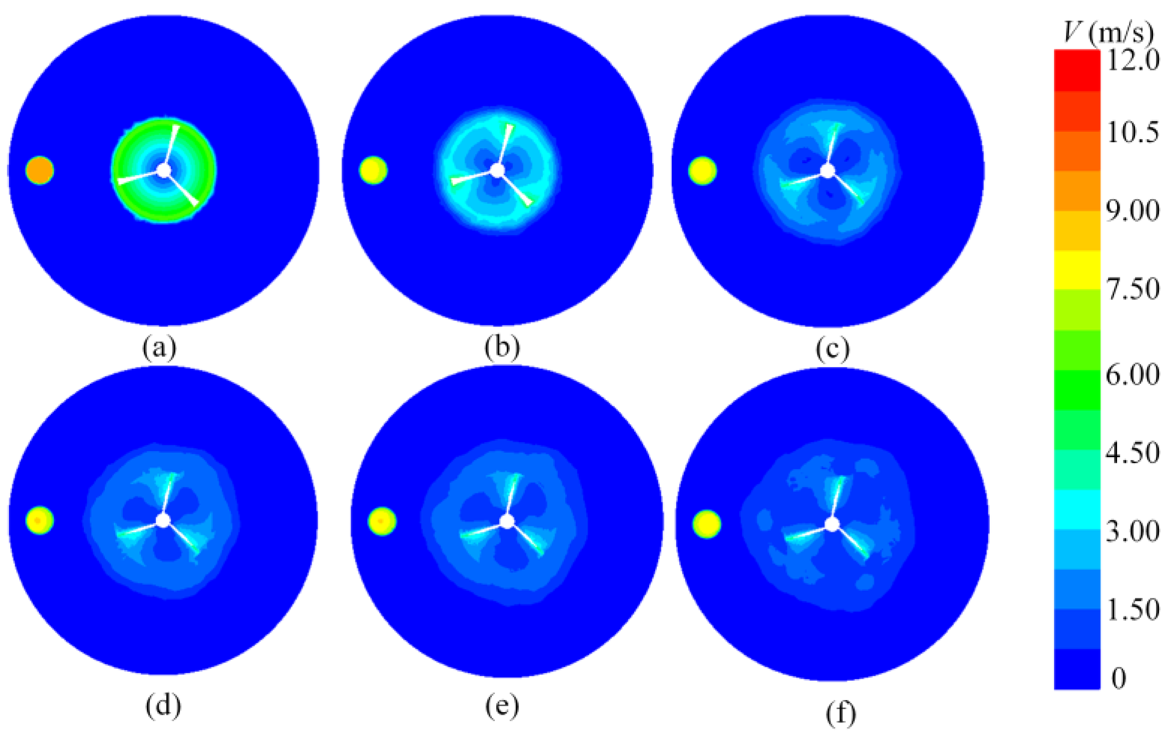
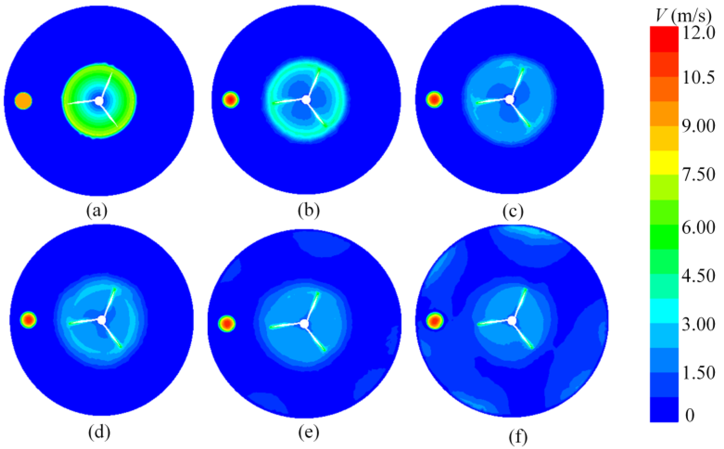
4.1. Gas–Liquid–Solid Three-Phase Flow Mixing Process

Based on the above model, the gas–liquid–solid three-phase flow mixing process was studied, and the flow field velocity and pressure changes during blade rotation were obtained, as shown in Figure 3 and Figure 4. As seen from the figures, with the rotation process of the impeller, a high-speed region is formed near the blade and a low-speed region between the blades. This indicates that in the whole stirring process, the material mixing degree near the blade is much better than that of the outflow field due to the high flow velocity near the impeller. At the same time, due to the influence of stirring speed, size of the stirring blade, and structure of the stirring blade, the flow field near the blade has a high-velocity gradient change, while the flow field away from the stirring blade has no significant change. Therefore, there is a low stirring speed area near the wall, which may lead to the deposition of particles.
By comparing the upper blade with the lower blade, it can be seen that the structure of the lower blade is more than three lower baffles than that of the upper blade. The size of the lower blade is more significant than that of the upper blade, so the velocity gradient change of the flow field is more prominent. Due to the larger size of the blade, the flow field around the blade has a larger range of high-speed zone, and the outer end of the blade has a stronger flow field disturbance ability, reflecting the better mixing effect of particle materials on the side. Therefore, in the study of material mixing, it is of great significance to consider increasing the blade size appropriately to provide greater disturbance velocity for the flow field, which is of great significance in improving the material mixing transport process.
To visually observe the characteristics of the flow field interacting with impeller rotation under inflation conditions, the velocity profile and static pressure profile of the whole flow field are given, as shown in Figure 5. Due to the large inflation velocity, the impeller rotation has little change in the flow field disturbance. The maximum velocity is set at 12 m/s to visually observe the flow field velocity and static pressure under the combined action of the two. As seen from the figure, when charging at the bottom of the central pipe, the flow field in the central area has the maximum velocity with the rotation of the lower impeller, and its value is 12.0 m/s. With the evolution of the flow field and the effect of impeller rotation, the velocity disturbance in the bottom center area increases. Under aeration, the flow velocity at the bottom diffuses around and forms a local upward flow trend near the wall surface. In the material conveying pipeline, by the negative pressure of the discharge port, the speed inside the pipeline is also enormous so that the particle physics near the pipe mouth can be quickly sucked away.
According to the flow field analysis results, the static pressure distribution profile of the impeller is obtained. The total pressure of the flow field is controlled by static and dynamic pressure. In the stirred flow field, due to the rotation of the stirred blade, the static pressure of the flow field has a significant pressure gradient change, as shown in Figure 6 and Figure 7. The plus and the minus sign represents the direction of the static pressure gradient. Under the influence of impeller rotation, the static pressure of the flow field also has a low-pressure region and a high-pressure region. There is a high-pressure region in the direction before blade rotation (counterclockwise rotation) and a low-pressure region after blade rotation. Outside the blade, the pressure gradient has no noticeable change, which reflects that the rotation of the blade mainly affects the change of the flow field around the blade. In Figure 7, the pressure variation range of the lower impeller is more prominent, indicating that the larger impeller size provides more excellent velocity disturbance to the flow field, resulting in the formation of more obvious annular characteristics of the pressure in the flow field. The above process can provide a greater driving force for particle suspension in the flow field and avoid particle material deposition at the bottom.
Figure 8 shows the static pressure profile of the fluid. As seen from the figure, at the initial moment, the pressure of the aerated pipe is relatively small, and with aeration, the pressure increases continuously. However, the pressure of the flow field has no noticeable change, showing a more uniform stratification. The pressure value is relatively large at the bottom of the mixing space, and at the upper part, the pressure of the flow field is slight. It indicates that the impeller disturbance effect of the upper part is small. Therefore, to improve the mixing process of materials in the mixing space, it is of great significance to choose the scale and structure of the bottom impeller reasonably.

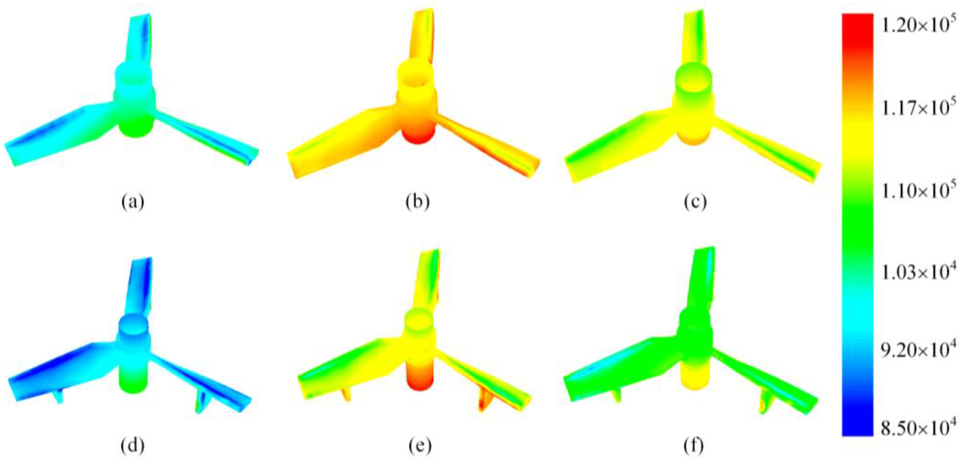
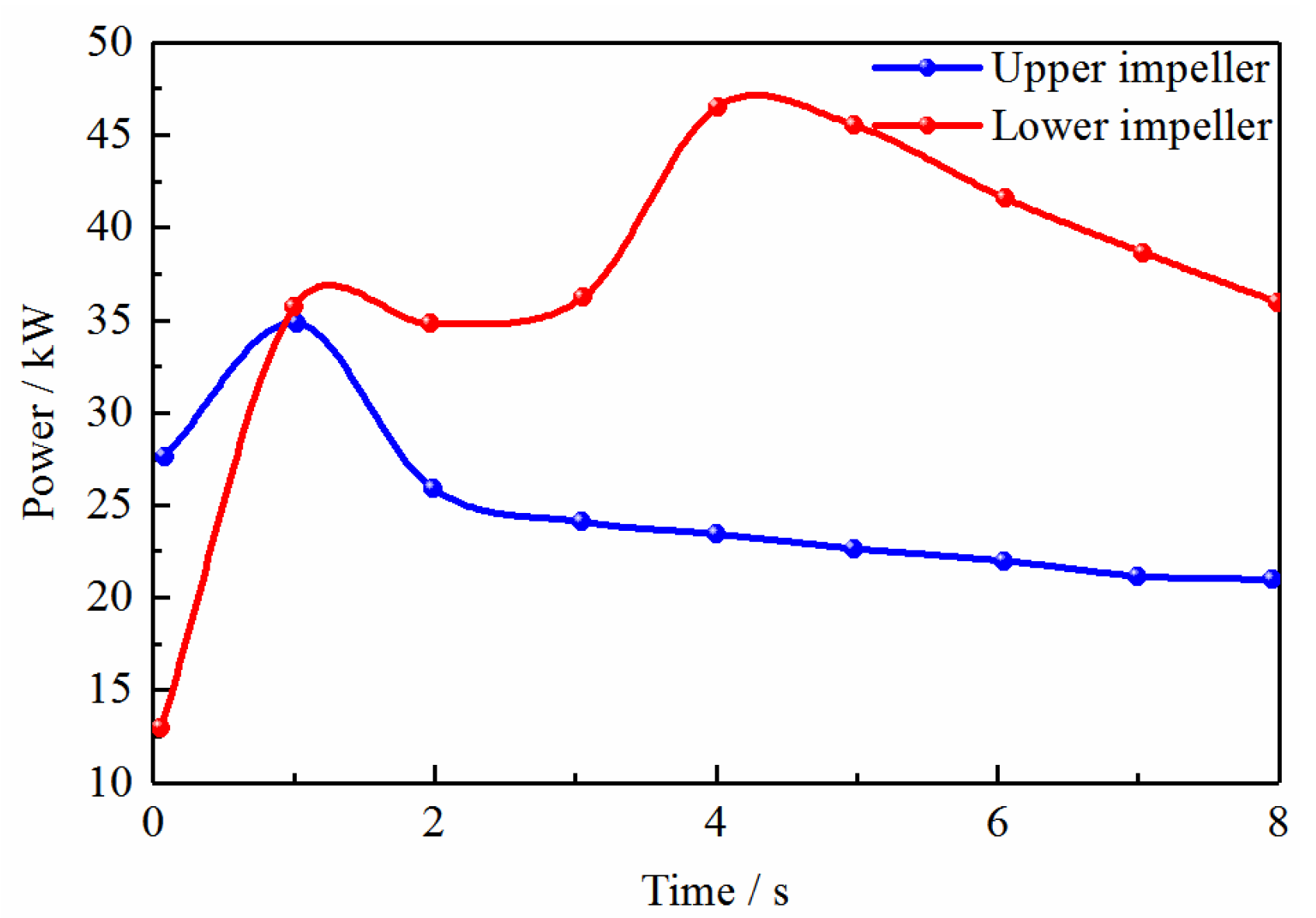
4.2. Bearing Power Calculation

Calculation of output shaft power is a common problem in industrial production. In this paper, the torque changes of the upper and lower impeller at different times in the moving process are obtained, respectively. The pressure load distribution of the impeller is shown in Figure 9. Due to the influence of many factors, such as fluid inertia force, particle settlement, and bottom-blowing effect in the stirring process, the impeller shows excellent changes in pressure load. Although there is no positive correlation between pressure load and torque, the coupling effects of many factors also lead to the fluctuation of impeller torque in the early stirring stage. The torque of the impeller is mainly affected by two aspects, one is the pressure load, and the other is the viscous force of the fluid boundary layer. The torque brought by each factor is shown in Table 1.
In this example, the torque the pressure load brings is the central part, and the proportion of the viscous force is about 1–2%. From the point of view of time, the pressure load torque of the upper impeller continues to decline, mainly due to the initial agitation. The impeller needs to overcome the fluid inertia force to do work. With the progress of agitation, the impeller rotation area velocity increases, and the need to overcome the inertia force decreases, so the pressure load torque decreases. On the other hand, affected by particle settlement, fluid density distribution is uneven, which also leads to the torque required by the upper impeller becoming smaller and the torque required by the lower impeller becoming larger. The effect of viscous force on the lower impeller changes little. The pressure load presents a trend of increasing first and then slowly decreasing, which may be because the scale of particle settlement effect in the early stage of agitation is larger than the scale of fluid inertia force reduction. In DEM simulation, the particles suspended in the flow field are also deposited to the lower half of the region at about 4 s. After that, under the influence of blade rotation and bottom blowing effect, the particle deposition effect was weakened. At the same time, the fluid inertia force was still reduced. Therefore, the torque of the lower impeller gradually decreased after 4 s.
The power calculation of the upper and lower impellers is shown in Figure 10. According to the internal situation of the flow field, taking the rotating shaft as the center, the power changes over time are calculated using statistics of the torque of the upper impeller and the lower impeller, respectively, as shown in the figure. The power value of the upper impeller varies in the range of 21~35 kW, among which the higher power of 1 s should be related to the amount of material around at this time and is greatly affected by the initial conditions and disturbance.
Then, the amount of material settlement, the amount of material around the impeller, decreases, and the power consumption decreases. In the actual project, if the material and the viscosity change cover the impeller, its power consumption is between 42~50 kW. The power consumption of the lower impeller with the material settlement sees an upward trend, affected by the bottom blowing and material settlement, power between 35~48 kW. As seen from the figure, the power peak of the upper impeller is 35 kW after a working period, stable to about 20~25 kW, and the peak power of the lower impeller is about 48 kW and about 35~45 kW after stability. When the two are added together, the peak power of the impeller is about 80 kW, and the stable power is 55~70 kW. The power may fluctuate to some extent, taking into account the changes in the viscosity of the medium and the additional resistance the actual motor drive overcomes. By referring to the relevant literature, it can be known from experience that given a power coefficient of 1.4~1.5 to ensure the increase in viscosity to overcome the power consumption caused by additional resistance, the peak starting power of the motor is 112~120 kW, and the power of the motor after the stable operation is 83~105 kW.

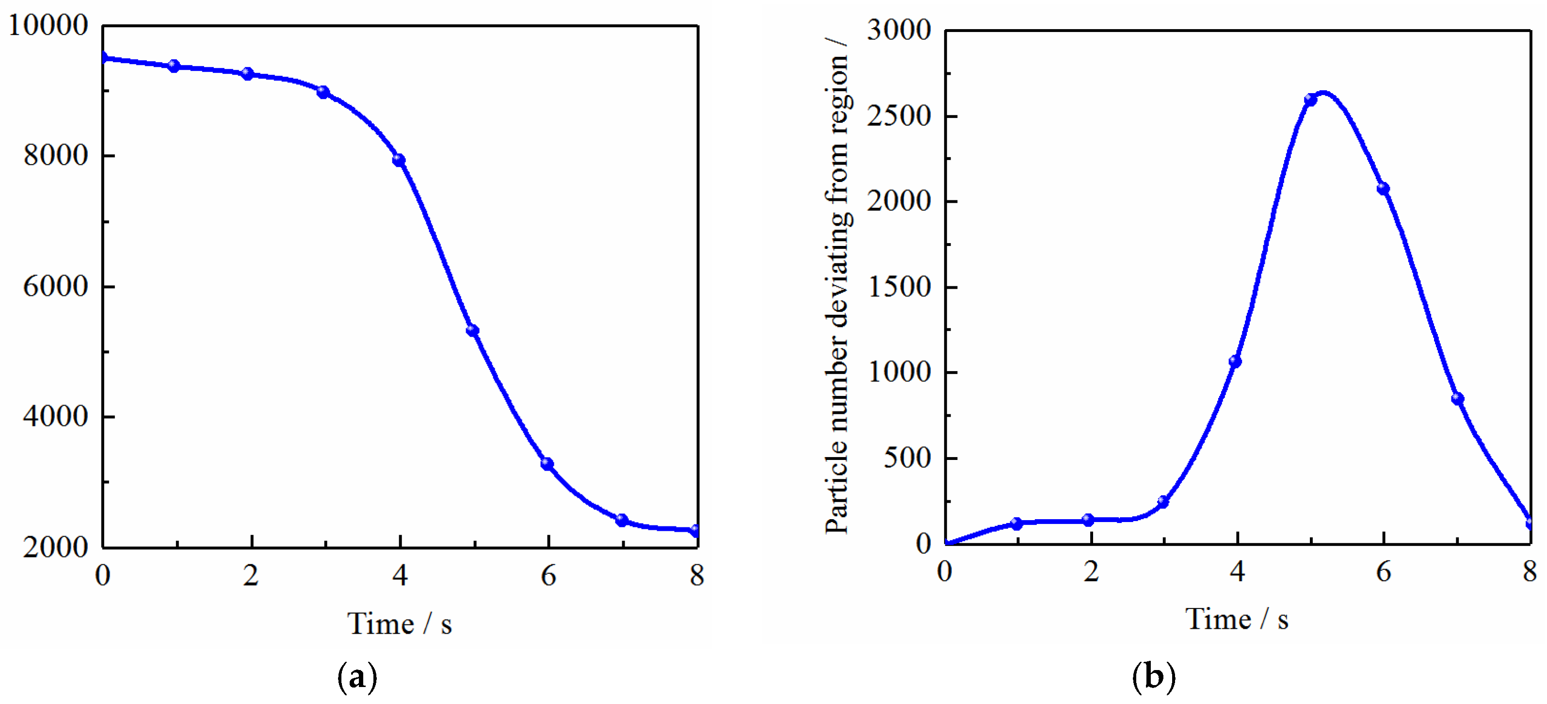
4.3. Evolution Law of Particle Flows

Figure 11 shows the dynamic evolution process of granular material corresponding to the flow field, including material feed, material extraction, rotation of the rotating shaft, and mixing under the standard conditions of a low blow. In Figure 11, particles from the top feed port enter the mixing space. The feeding volume is 990 m3/h, and the bottom impeller-covered volume is about 483 m3 (h = 4 m). According to the results of the first 8 s of the value, blowing air at the bottom is more prominent, resulting in the apparent floating of particles at the bottom. For the specified initial region, many particles will be suspended after 3 s~4 s, and the number of particles remaining in the initial region is significantly reduced, as shown in Figure 12a. According to the rotation period of the impeller of 2 s, the whole flow field is basically in a relatively stable state in about two cycles. That is, the flow field is stable after 4 s. In Figure 12a, from 4 s to 6 s, the particles in the initial region are reduced from 8000 to 3200, which is more than 3/5. Meanwhile, in this 2 s period, the number of particles leaving the region is the largest, as shown in Figure 12b. Therefore, it can be considered that under the condition of a stable flow field, the stagnation time of particles in the bottom region is about 2 s. They will be suspended and discharged under the disturbance of the flow field and bottom blowing. In the feeding process, the rotating flow field affected by the upper impeller will suck part of the material into the upper flow field. At the same time, the flow field disturbed by the lower impeller will also suspend many materials, and the material at the bottom will be suspended for 2 s.
Figure 13 shows the dynamic evolution process of granular material in the coupling process and gives the time profile of velocity change and velocity vector. Through observation, it can be seen that at an early stage of the mixing process, the material mainly suffers from the action of gravity and appears in the settling motion. In the process of blade rotation, the velocity of granular material near the blade changes obviously, and its velocity gradient changes significantly, which is consistent with the velocity variation near the blade in the flow field. In addition, when the particle material settles and accumulates to a certain extent, the particle movement is blocked, and the stirring speed of the particle material near the blade is reduced. At this point, the effect of mixing will be significantly reduced near the wall; near the particle material, it is also challenging to stir more fully. We can see the inflation situation and the bottom material agitation. At the same time, under the suction of negative pressure, the material will also be pumped away by the discharge pipe.

5. Conclusions

Three-phase particle flow mixing transport course is essential for improving lithium battery dispersion and chemical material extraction. This paper proposes a CFD-DEM coupling-based three-phase particle flow modeling approach to study the mixing transport mechanism. The related research work has been completed, and the following conclusions have been obtained:
(1)
A three-phase particle flow dynamic model is built based on the coupled CFD-DEM method. An interphase coupling solution method is utilized to solve the interaction effects of the fluid and particle. The particle flow mixing transfer mechanism is revealed via the evolution laws of relevant physical characteristics (such as velocity, pressure, particle vector, etc.);
(2)
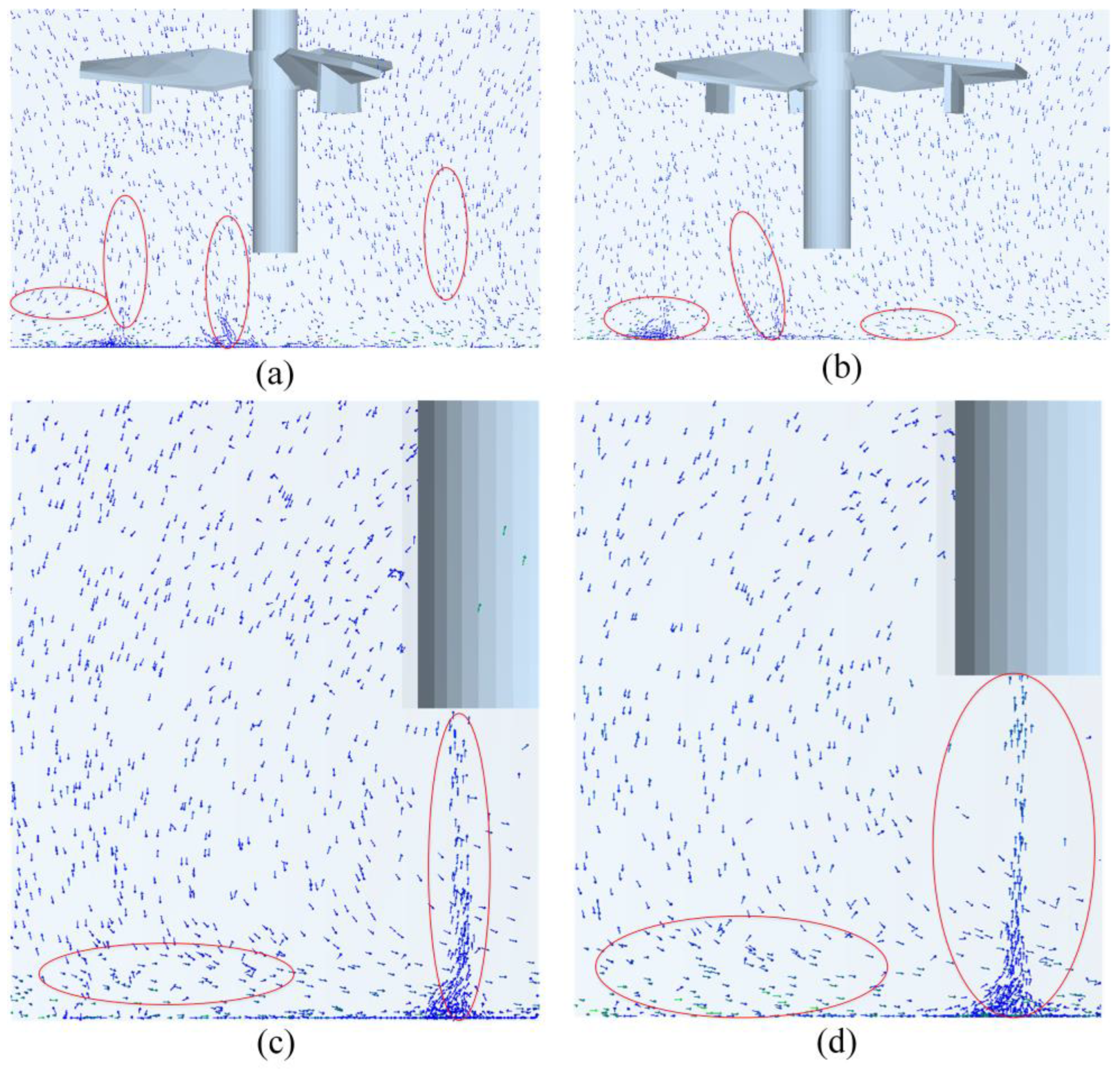
The flow field near the blade has a high-velocity gradient change due to the influence of stirring speed, the stirring blade’s size, and structure. A low stirring speed area near the wall occurs and may lead to the deposition of particles. The effect of impeller rotation, the velocity disturbance in the bottom center area, increases. Under aeration, the flow velocity at the bottom diffuses around and forms a local upward flow trend near the wall surface. The speed inside the pipeline is also enormous, so the particle physics near the pipe mouth can quickly be sucked away;
(3)
As the particle material settles and accumulates to a certain extent, the particle movement is blocked, and the stirring speed of the particle material near the blade is reduced. The flow field disturbed by the lower impeller will also suspend many materials, and the material at the bottom will be suspended for 2 s. The mixing effect of the particle material will be reduced near the wall. It can provide a valuable reference for particle flow transport and pattern identification and support technical support for homogenate mixing, chemical extraction, and pharmacy process regulation.
The mixing transport process of three-phase particle flows is a complex turbulent mechanic matter, but it might be controlled by air inflation. Subsequent studies will explore facets of the lattice Boltzmann method (LBM-DEM) coupled solution and fractal dimensions for multiphase flows and expand its application in chemical, medical, food, and other fields.

Author Contributions

Conceptualization, G.Z. and M.G.; article identification, screening, retrieval, selection, and analysis, G.Z., J.C., L.Z. and M.G.; formal analysis and investigation, G.Z. and M.G.; writing—original draft preparation, G.Z., J.C. and M.G.; tables and figures generation, G.Z. and M.G.; review and editing, G.Z. and M.G.; supervision, M.G.; funding acquisition, M.G. and J.C. All authors have read and agreed to the published version of the manuscript.

Funding

This research work was supported by the Open Research Project of Robot Technology and Intelligent Manufacturing Equipment Engineering Laboratory of Jiangsu Province under the Grant SDGC2140.

Institutional Review Board Statement

Not applicable.

Informed Consent Statement

Not applicable.

Data Availability Statement

Not applicable.

Conflicts of Interest

The authors declare no conflict of interest.

References

  1. Li, L.; Qi, H.; Yin, Z.; Li, D.; Zhu, Z.; Tangwarodomnukun, V.; Tan, D. Investigation on the multiphase sink vortex Ekman pumping effects by CFD-DEM coupling method. Powder Technol. 2020, 360, 462–480. [Google Scholar] [CrossRef]
  2. Yuan, W.L.; Zhang, S.J.; Su, C.G. Flow analysis on carbonaceous deposition of heavy oil droplets and catalyst particles for coking formation process. Energy 2022, 252, 124025. [Google Scholar] [CrossRef]
  3. Jin, X.; Liu, B.; Liao, S.; Cheng, C.; Zhang, Y.; Zhao, Z.; Lu, J. Wasserstein metric-based two-stage distributionally robust optimization model for optimal daily peak shaving dispatch of cascade hydroplants under renewable energy uncertainties. Energy 2022, 260, 125107. [Google Scholar] [CrossRef]
  4. Li, L.; Tan, D.; Yin, Z.; Wang, T.; Fan, X.; Wang, R. Investigation on the multiphase vortex and its fluid-solid vibration characters for sustainability production. Renew. Energy 2021, 175, 887–909. [Google Scholar] [CrossRef]
  5. Wang, J.; Gao, S.; Tang, Z.; Tan, D.; Cao, B.; Fan, J. A context-aware recommendation system for improving manufacturing process modeling. J. Intell. Manuf. 2021, 34, 1347–1368. [Google Scholar] [CrossRef]
  6. Tan, D.; Li, L.; Yin, Z.; Li, D.; Zhu, Y.; Zheng, S. Ekman boundary layer mass transfer mechanism of free sink vortex. Int. J. Heat Mass Transfer. 2020, 150, 119250. [Google Scholar] [CrossRef]
  7. Li, L.; Tan, Y.; Xu, W.; Ni, Y.; Yang, J.; Tan, D. Fluid-induced transport dynamics and vibration patterns of multiphase vortex in the critical transition states. Int. J. Mech. Sci. 2023, 252, 108376. [Google Scholar] [CrossRef]
  8. Li, L.; Gu, Z.; Xu, W.; Tan, Y.; Fan, X.; Tan, D. Mixing mass transfer mechanism and dynamic control of gas-liquid-solid multiphase flow based on VOF-DEM coupling. Energy 2023, 272, 127015. [Google Scholar] [CrossRef]
  9. Li, L.; Li, Q.H.; Ni, Y.S.; Wang, C.Y.; Tan, Y.F.; Tan, D.P. Critical penetrating vibration evolution behaviors of the gas-liquid coupled vortex flow. Energy, 2023; in press. [Google Scholar]
  10. Li, L.; Wan, Y.; Lu, J.; Fang, H.; Yin, Z.; Wang, T.; Wang, R.; Fan, X.; Zhao, L.; Tan, D. Lattice Boltzmann Method for Fluid-Thermal Systems: Status, Hotspots, Trends and Outlook. IEEE Access 2020, 8, 27649–27675. [Google Scholar] [CrossRef]
  11. Xu, W.; Tan, Y.; Li, M.; Sun, J.; Xie, D.; Liu, Z. Effects of surface vortex on the drawdown and dispersion of floating particles in stirred tanks. Particuology 2020, 49, 159–168. [Google Scholar] [CrossRef]
  12. Bao, Y.; Wang, B.; Lin, M.; Gao, Z.; Yang, J. Influence of impeller diameter on overall gas dispersion properties in a sparged multi-impeller stirred tank. Chin. J. Chem. Eng. 2015, 23, 890–896. [Google Scholar] [CrossRef]
  13. Gu, D.; Liu, Z.; Xie, Z.; Li, J.; Tao, C.; Wang, Y. Numerical simulation of solid-liquid suspension in a stirred tank with a dual punched rigid-flexible impeller. Adv. Powder Technol. 2017, 28, 2723–2734. [Google Scholar] [CrossRef]
  14. Blais, B.; Bertrand, F. CFD-DEM investigation of viscous solid-liquid mixing: Impact of particle properties and mixer characteristics. Chem. Eng. Res. Des. 2017, 118, 270–285. [Google Scholar] [CrossRef]
  15. Kou, B.; Hou, Y.; Fu, W.; Yang, N.; Liu, J.; Xie, G. Simulation of Multi-Phase Flow in Autoclaves Using a Coupled CFD-DPM Approach. Processes 2023, 11, 890. [Google Scholar] [CrossRef]
  16. Brazhenko, V.; Qiu, Y.; Mochalin, I.; Zhu, G.; Cai, J.-C.; Wang, D. Study of hydraulic oil filtration process from solid admixtures using rotating perforated cylinder. J. Taiwan Inst. Chem. Eng. 2022, 141, 104578. [Google Scholar] [CrossRef]
  17. Li, L.; Tan, D.; Wang, T.; Yin, Z.; Fan, X.; Wang, R. Multiphase coupling mechanism of free surface vortex and the vibration-based sensing method. Energy 2021, 216, 119136. [Google Scholar] [CrossRef]
  18. Tan, D.-P.; Li, L.; Zhu, Y.-L.; Zheng, S.; Yin, Z.-C.; Li, D.-F. Critical penetration condition and Ekman suction-extraction mechanism of a sink vortex. J. Zhejiang Univ. Sci. A 2019, 20, 61–72. [Google Scholar] [CrossRef]
  19. Li, L.; Lu, B.; Xu, W.-X.; Gu, Z.-H.; Yang, Y.-S.; Tan, D.-P. Mechanism of multiphase coupling transport evolution of free sink vortex. Acta Phys. Sin. 2023, 72, 034702. [Google Scholar] [CrossRef]
  20. Tan, D.-P.; Ni, Y.-S.; Zhang, L.-B. Two-phase sink vortex suction mechanism and penetration dynamic characteristics in ladle teeming process. J. Iron Steel Res. Int. 2017, 24, 669–677. [Google Scholar] [CrossRef]
  21. Zheng, S.; Yu, Y.; Qiu, M.; Wang, L.; Tan, D. A modal analysis of vibration response of a cracked fluid-filled cylindrical shell. Appl. Math. Model. 2021, 91, 934–958. [Google Scholar] [CrossRef]
  22. Yin, Z.C.; Ni, Y.S.; Li, L.; Wang, T.; Wu, J.F.; Li, Z.; Tan, D.P. Numerical modelling and experimental investigation of a two-phase sink vortex and its fluid-solid vibration characteristics. J. Zhejiang Univ. Sci. A, 2022; in press. [Google Scholar]
  23. Li, S.; Chen, R.; Wang, H.; Liao, Q.; Zhu, X.; Wang, Z.; He, X. Numerical investigation of the moving liquid column coalescing with a droplet in triangular microchannels using CLSVOF method. Sci. Bull. 2015, 60, 1911–1926. [Google Scholar] [CrossRef]
  24. Tan, D.P.; Tao, Y.; Zhao, J. Free sink vortex Ekman suction-extraction evolution mechanism. Acta Phys. Sin. 2016, 65, 054701. [Google Scholar]
  25. Zhang, B.; Li, B.; Fu, S.; Mao, Z.; Ding, W. Vortex-Induced Vibration (VIV) hydrokinetic energy harvesting based on nonlinear damping. Renew. Energy 2022, 195, 1050–1063. [Google Scholar] [CrossRef]
  26. Park, I.S.; Sohn, C.H. Experimental and numerical study on air cores for cylindrical tank draining. Int. Commun. Heat Mass Transf. 2011, 38, 1044–1049. [Google Scholar] [CrossRef]
  27. Fan, X.; Guo, K.; Wang, Y. Toward a high performance and strong resilience wind energy harvester assembly utilizing flow-induced vibration: Role of hysteresis. Energy 2022, 251, 123921. [Google Scholar] [CrossRef]
  28. Zeng, Y.; Shi, W.; Michailides, C.; Ren, Z.; Li, X. Turbulence model effects on the hydrodynamic response of an oscillating water column (OWC) with use of a computational fluid dynamics model. Energy 2022, 261, 124926. [Google Scholar] [CrossRef]
  29. Stroh, A.; Daikeler, A.; Nikku, M.; May, J.; Alobaid, F.; von Bohnstein, M.; Ströhle, J.; Epple, B. Coarse grain 3D CFD-DEM simulation and validation with capacitance probe measurements in a circulating fluidized bed. Chem. Eng. Sci. 2019, 196, 37–53. [Google Scholar] [CrossRef]
  30. Wang, T.; Wang, C.; Yin, Y.; Zhang, Y.; Li, L.; Tan, D. Analytical approach for nonlinear vibration response of the thin cylindrical shell with a straight crack. Nonlinear Dyn. 2023, 111, 10957–10980. [Google Scholar] [CrossRef]
  31. Zhou, L.; Zhao, Y. CFD-DEM simulation of fluidized bed with an immersed tube using a coarse-grain model. Chem. Eng. Sci. 2020, 231, 116290. [Google Scholar] [CrossRef]
  32. Kang, Q.; He, D.; Zhao, N.; Feng, X.; Wang, J. Hydrodynamics in unbaffled liquid-solid stirred tanks with free surface studied by DEM-VOF method. Chem. Eng. J. 2020, 386, 122846. [Google Scholar] [CrossRef]
  33. Zheng, M.; Han, D.; Peng, T.; Wang, J.; Gao, S.; He, W.; Li, S.; Zhou, T. Numerical investigation on flow induced vibration performance of flow-around structures with different angles of attack. Energy 2021, 244, 122607. [Google Scholar] [CrossRef]
  34. Singh, N.K.; Premachandran, B. A coupled level set and volume of fluid method on unstructured grids for the direct numerical simulations of two-phase flows including phase change. Int. J. Heat Mass Transf. 2018, 122, 182–203. [Google Scholar] [CrossRef]
  35. Tan, D.-P.; Li, L.; Zhu, Y.-L.; Zheng, S.; Ruan, H.-J.; Jiang, X.-Y. An Embedded Cloud Database Service Method for Distributed Industry Monitoring. IEEE Trans. Ind. Inform. 2017, 14, 2881–2893. [Google Scholar] [CrossRef]
  36. He, X.; Xu, H.; Li, W.; Sheng, D. An improved VOF-DEM model for soil-water interaction with particle size scaling. Comput. Geotech. 2020, 128, 103818. [Google Scholar] [CrossRef]
  37. Li, L.; Yang, Y.-S.; Xu, W.-X.; Lu, B.; Gu, Z.-H.; Yang, J.-G.; Tan, D.-P. Advances in the Multiphase Vortex-Induced Vibration Detection Method and Its Vital Technology for Sustainable Industrial Production. Appl. Sci. 2022, 12, 8538. [Google Scholar] [CrossRef]
  38. Son, J.H.; Sohn, C.H.; Park, I.S. Numerical study of 3-D air core phenomenon during liquid draining. J. Mech. Sci. Technol. 2015, 29, 4247–4257. [Google Scholar] [CrossRef]
  39. Tan, Y.; Ni, Y.; Wu, J.; Li, L.; Tan, D. Machinability evolution of gas–liquid-solid three-phase rotary abrasive flow finishing. Int. J. Adv. Manuf. Technol. 2023, 1–20. [Google Scholar] [CrossRef]
  40. Zheng, G.; Shi, J.; Li, L.; Li, Q.; Gu, Z.; Xu, W.; Lu, B.; Wang, C. Fluid-Solid Coupling-Based Vibration Generation Mechanism of the Multiphase Vortex. Processes 2023, 11, 568. [Google Scholar] [CrossRef]
  41. Song, Y.; Pan, Z.; Yu, T.; Zhou, S.; Li, Y.; Jin, W.; Gao, Z.; Ma, Y. Nanoindentation characterization on competing propagation between the transgranular and intergranular cracking of 316H steel under creep-fatigue loading. Fatigue Fract. Eng. Mater. Struct. 2023, 46, 2258–2271. [Google Scholar] [CrossRef]
  42. Zheng, G.; Gu, Z.; Xu, W.; Lu, B.; Li, Q.; Tan, Y.; Wang, C.; Li, L. Gravitational Surface Vortex Formation and Suppression Control: A Review from Hydrodynamic Characteristics. Processes 2023, 11, 42. [Google Scholar] [CrossRef]
  43. Tan, Y.; Ni, Y.; Xu, W.; Xie, Y.; Li, L.; Tan, D. Key technologies and development trends of the soft abrasive flow finishing method. J. Zhejiang Univ. Sci. A 2023, 1–20. [Google Scholar] [CrossRef]
  44. Li, L.; Xu, W.; Tan, Y.; Yang, Y.; Yang, J.; Tan, D. Fluid-induced vibration evolution mechanism of multiphase free sink vortex and the multi-source vibration sensing method. Mech. Syst. Signal Process. 2023, 189, 110058. [Google Scholar] [CrossRef]
  45. Wu, L.; Gong, M.; Wang, J. Development of a DEM–VOF Model for the Turbulent Free-Surface Flows with Particles and Its Application to Stirred Mixing System. Ind. Eng. Chem. Res. 2018, 57, 1714–1725. [Google Scholar] [CrossRef]
Figure 1. Structure diagram of the mixing tank. (a) Overall structure diagram. (b) Local structure diagram of upper blade. (c) Local structure diagram of the lower blade.
Processes 11 01619 g001
Figure 2. Mesh division of the mixing vessel. (a) Overall grid diagram. (b) Impeller local encryption diagram.
Processes 11 01619 g002
Figure 3. Velocity distribution of the upper impeller. (a) t = 0 s. (b) t = 1.60 s. (c) t = 3.20 s. (d) t = 4.80 s. (e) t = 6.40 s. (f) t = 8.00 s.
Processes 11 01619 g003
Figure 4. Velocity distribution of the lower impeller. (a) t = 0 s. (b) t = 1.60 s. (c) t = 3.20 s. (d) t = 4.80 s. (e) t = 6.40 s. (f) t = 8.00 s.
Processes 11 01619 g004
Figure 5. Velocity profile of the fluid domain. (a) t = 0 s. (b) t = 1.60 s. (c) t = 3.20 s. (d) t = 4.80 s. (e) t = 6.40 s. (f) t = 8.00 s.
Processes 11 01619 g005
Figure 6. Static pressure distribution of the upper impeller. (a) t = 0 s. (b) t = 1.60 s. (c) t = 3.20 s. (d) t = 4.80 s. (e) t = 6.40 s. (f) t = 8.00 s.
Processes 11 01619 g006
Figure 7. Static pressure distribution of the lower impeller. (a) t = 0 s. (b) t = 1.60 s. (c) t = 3.20 s. (d) t = 4.80 s. (e) t = 6.40 s. (f) t = 8.00 s.
Processes 11 01619 g007
Figure 8. Static pressure profile of the fluid domain. (a) t = 0 s. (b) t = 1.60 s. (c) t = 3.20 s. (d) t = 4.80 s. (e) t = 6.40 s. (f) t = 8.00 s.
Processes 11 01619 g008
Figure 9. Pressure load distribution of upper and lower impeller. (a) t = 1 s. (b) t = 4 s. (c) t = 8 s. (d) t = 1 s. (e) t = 4 s. (f) t = 8 s. Subfigure (ac) represents the upper impeller, and subfigure (df) represents the lower impeller.
Processes 11 01619 g009
Figure 10. Power change curve of the upper and lower impellers.
Processes 11 01619 g010
Figure 11. The evolution process of particle material velocity.
Processes 11 01619 g011
Figure 12. Particle number variation curves. (a) Changes in the number of particles in the initial region. (b) The number of particles leaving the initial region per second.
Processes 11 01619 g012
Figure 13. Partial profile of material velocity vector. The subfigure (a,b) represents the partial profile near the filled hole of t = 3.50 s and 4.00 s. The subfigure (c,d) represents the partial profile near the discharge hole of t = 3.50 s and 4.00 s.
Processes 11 01619 g013
Table 1. Changes of impeller torque at rated speed.
ImpellerTimePressure Loading
(N·m)
Viscous Force Action
(N·m)
Total Moment
(N·m)
1 s12,653.13679.33912,732.475
2 s9424.39385.6369510.029
3 s8755.41884.0498839.467
4 s8447.32583.1668530.491
Upper5 s8241.53284.7548326.287
6 s7947.01388.3728035.385
7 s7729.40192.7817822.182
8 s7658.06696.3787754.444
1 s12,998.457251.77913,250.237
2 s9069.175261.8699331.044
3 s13,124.848262.51513,387.363
Lower4 s16,885.797220.34717,106.144
5 s16,595.645217.65316,813.298
6 s15,205.691229.58715,435.278
7 s13,960.441242.00114,202.442
8 s13,170.671259.89913,430.572
Disclaimer/Publisher’s Note: The statements, opinions and data contained in all publications are solely those of the individual author(s) and contributor(s) and not of MDPI and/or the editor(s). MDPI and/or the editor(s) disclaim responsibility for any injury to people or property resulting from any ideas, methods, instructions or products referred to in the content.

