Article

Using Ant Colony Optimization as a Method for Selecting Features to Improve the Accuracy of Measuring the Thickness of Scale in an Intelligent Control System

by
Abdulilah Mohammad Mayet
1,
V. P. Thafasal Ijyas
1,
Javed Khan Bhutto
1,
John William Grimaldo Guerrero
2,*,
Neeraj Kumar Shukla
1,
Ehsan Eftekhari-Zadeh
3,* and
Hala H. Alhashim
4
1
Electrical Engineering Department, King Khalid University, Abha 61411, Saudi Arabia
2
Department of Energy, Universidad de la Costa, Barranquilla 080001, Colombia
3
Institute of Optics and Quantum Electronics, Abbe Center of Photonics, Friedrich Schiller University Jena, 07743 Jena, Germany
4
Department of Physics, College of Science, Imam Abdulrahman Bin Faisal University, Dammam 31441, Saudi Arabia
*
Authors to whom correspondence should be addressed.
Processes 2023, 11(6), 1621; https://doi.org/10.3390/pr11061621
Submission received: 23 April 2023 / Revised: 16 May 2023 / Accepted: 18 May 2023 / Published: 26 May 2023

Abstract

:
The scaling of oil pipelines over time leads to issues including diminished flow rates, wasted energy, and decreased efficiency. To take appropriate action promptly and avoid the aforementioned issues, it is crucial to determine the precise value of the scale within the pipe. Non-invasive gamma attenuation systems are one of the most accurate detection methods. To accomplish this goal, the Monte Carlo N Particle (MCNP) algorithm was used to simulate a scale thickness measurement system, which included two sodium iodide detectors, a dual-energy gamma source (241 Am and 133 Ba radioisotopes), and a test pipe. Water, gas, and oil were all used to mimic a three-phase flow in the test pipe, with the volume percentages ranging from 10% to 80%. Moreover, a scale ranging in thickness from 0 to 3 cm was inserted into the pipe, gamma rays were shone on the pipe, and on the opposite side of the pipe, photon intensity was measured by detectors. There were 252 simulations run. Fifteen time and frequency characteristics were derived from the signals collected by the detectors. The ant colony optimisation (ACO)-based approach is used to pick the ideal inputs from among the extracted characteristics for determining the thickness of the scale within the pipe. This technique led to the introduction of thirteen features that represented the ideal combination. The features introduced by ACO were introduced as inputs to a multi-layer perceptron (MLP) neural network to predict the scale thickness inside the oil pipe in centimetres. The maximum error found in calculating scale thickness was 0.017 as RMSE, which is a minor error compared to earlier studies. The accuracy of the present study in detecting scale thickness has been greatly improved by using the ACO to choose the optimal features.

1. Introduction

The buildup of scale in oil-transport pipes has resulted in a variety of issues in oil fields across the world. When scale builds up in a pipeline, the effective cross-sectional area becomes smaller. This makes it harder for petroleum products to move through the pipeline. Because of this part, pumps and other machines cannot work properly. Downtime catastrophes, damaged oil gear, higher maintenance costs, and decreased efficiency may result from an increase in the amount of scale in the pipeline if it is not identified in a timely manner. To go forward while scale is present, it is important to utilise a control system with features such as scale thickness detection. For calculating the many features of a two-phase flow, gamma-ray attenuation systems are widely regarded as the benchmark by scientists [1,2,3,4,5,6,7,8]. The apparatus employed by the researchers in [1] consisted of a cesium source, a test pipe, and two sodium iodide detectors. The RBF neural network was fed the counts from two detectors to predict a two-phase flow property with three regimes: bubbly, stratified, and annular. By tallying up these numbers, they were able to make educated guesses about the volume fractions and classify the flow patterns. One alternative neural network paradigm is the polynomial neural network, often known as the group method of data handling (GMDH). The GMDH approach uses an inductive self-organizing technique to estimate black box models with unknown relationships between variables. Artificial neural networks of the GMDH type were utilised by Roshni et al. [2] to identify the volume percentages and flow regimes by training on the unbalanced data. The impressive precision of the technology was used to justify the massive computing costs. The flow regime and volumetric percentage were previously detected by Roshani et al. [3], using a cobalt-60 source and a NaI detector, but the parameters were not precisely measured due to the erroneous characteristics being extracted. Researchers in 2019 used the Jaya optimisation algorithm to provide predictions about the volumetric percentages [4]. Sattari and colleagues set up a system for precise volume percentage calculation and flow regime categorization using 2 NaI detectors, a 137Cs radioisotope, and a tube [5]. In subsequent research, they looked into the viability of using GMDH neural networks to detect distinct flow regimes and forecast volume fractions [6]. This research accurately calculated the volume percentage; however, it paid little attention to the quantity of scale in the pipe. Ba-133 and Cs-137 are used to measure the thickness of the scale in the oil pipe [7]. An RBF neural network was trained using data obtained from a simulation of the two-phase flow in various regimes, including information on detector properties for both transmission and scattering detectors. The RMSE for their predicted scale thickness was less than 0.22; therefore, their hard work paid off. 133 Ba and 241 Am were used to analyze the scale layer in an oil pipe in recent research. It was proposed that the photopeaks of 133 Ba and 241 Am from two detectors be used as inputs to the RBF neural network after modelling the three-phase flow in annular regimes. Eventually, they achieved an RMSE of less than 0.09 when estimating the thickness of scales [8]. Always-on, radioisotope-based energy sources have drawbacks, including the necessity for personnel to wear protective clothing and transportation constraints. Hence, X-ray tube research into measuring multiphase flow properties has gained traction in recent years [9,10,11,12]. X-rays and a NaI detector were used to determine the flow regime and volume fraction of two-phase flows in [9]. Two multilayer perceptron networks were trained using the detector’s signal timing properties. Models of a homogeneous flow, an annular flow, and a stratified flow were used to examine three-phase flows at varying volume fractions in [10]. Moreover, three RBF networks were trained using the input signals’ rather exact frequency characteristics. In [11], the MCNP method was used to model the X-ray tube’s core as it passed through a mixture of four petroleum products blended in pairs of varying concentrations. Three multilayer perceptron neural networks were fed the recorded signals, and their output was a prediction of the volume distribution of the three products. The fourth product’s volume ratio was easily determined after the volume ratios of the previous three were known. The presented method foresaw the objects’ types and quantities, but it lacked feature extraction techniques and therefore could not be very precise. Balubaid et al. [12] looked at the use of wavelet transformations as a method of feature extraction to expand previous studies [11]. The computing load was optimised, and accuracy was enhanced as a result of this effort. Large-scale combinatorial issues and nonlinear problems are beyond the capabilities of traditional optimisation techniques. Therefore, optimisation techniques based on metaheuristics have been presented. The nine categories used to assess general-purpose metaheuristic methodologies are as follows: biological, physical, social, musical, chemical, athletic, mathematical, swarm, and hybrid. Recent studies on plants have shown that they are capable of complex behaviours indicative of intelligence. Therefore, it is postulated that plants have some kind of neurological system. Algorithms and software programmes related to plant intelligence were compiled and analysed in [13]. These algorithms include the Flower Pollination Algorithm, Invasive Weed optimisation, Paddy Field Algorithm, Root Mass optimisation Algorithm, Artificial Plant optimisation Algorithm, Sapling Growing Up Algorithm, Photosynthetic Algorithm, Plant Growth Optimisation, Root Growth, Strawberry Algorithm as Plant Propagation Algorithm, Runner Root Algorithm, Path Planning Algorithm, and Rooted Tree optimisation. Due to the attitude of always seeking the best and the lack of the most efficient algorithm for all sorts of issues, new techniques or new versions of current methods are offered to test their ability to handle very complicated optimisation challenges. Recent work has presented two methods that seem to be light-based intelligent optimisation algorithms; these are ray optimisation and optics-inspired optimisation [14]. The principles of light refraction and reflection serve as inspiration for modern intelligent search and optimisation algorithms.
Most of the research described above has a big problem: it does not employ feature extraction and feature selection techniques that could be used to improve the performance of an artificial neural network. In order to solve this problem, a technique for extracting time-domain and frequency-domain characteristics and choosing the most useful characteristic using ant colony optimisation (ACO) has been presented in this study. Major contributions of current research are listed below.
  • Examining the time and frequency characteristics simultaneously in order to determine the thickness of the scale layer.
  • Using feature selection techniques based on the ACO algorithm to determine effective features.
  • Significant increase in the accuracy of the detection system by using appropriate specifications.
  • Reducing the amount of computation applied to the neural network by selecting the appropriate features in a manual process.
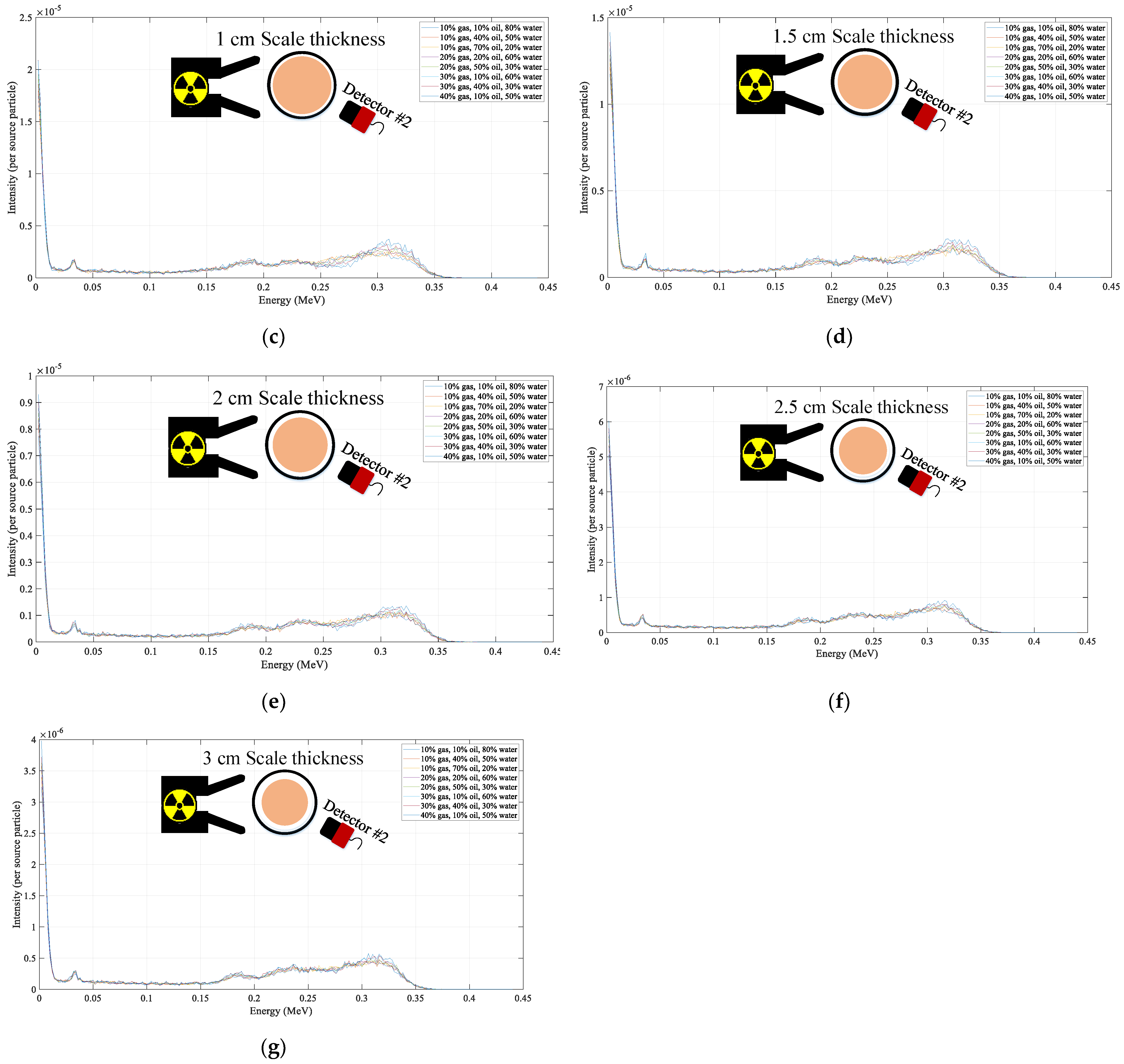
Figure 1 shows the general implementation process of the current research. The organization of this article is that first the detection system is simulated using MCNP code. Different thicknesses of the scale layer are investigated in this simulation. The detector signals are collected and labelled. In the next step, the received signals were analyzed and several time and frequency characteristics were extracted from the collected signals. In the next section, using the feature selection method based on the ACO algorithm, a combination of features that can determine the thickness of the scale with high accuracy is introduced. In the next section, the introduced features are applied as inputs to the MLP neural network, and a neural network is trained that can predict the scale thickness with high accuracy. In the last two parts, the results and conclusions of the current research will be presented.

2. Simulation Setup

Up to 1 TeV/nucleon, the MCNP (Monte Carlo N-Particle) code might be used to transport neutrons, photons, electrons, ions, and many other fundamental particles. Particles are moved through a three-dimensional model of a material, and the user chooses the surfaces at the first, second, and fourth levels of detail. Another option is to build complex geometry by putting a mesh inside a constructive solid geometry cell. This could be used with external structured and unstructured meshes to describe the geometry of the problem in a way that is a mix of the two. Models of physics and tables of nuclear and atomic data are used to simulate the physics of each encounter while the ship is in transit. Nuclear and atomic data tabulated for this energy range is often used to predict the effects of low-energy interactions between projectile particles (such as neutrons, photons, and light ions) and target nuclei. Academics have shown an ongoing fascination with modelling X-ray or gamma-radiation-using structures using the MCNP method [15,16,17,18]. The methodology presented in the current research was simulated using the MCNP code [19]. The framework proposed by the research revolves around the radioactive isotopes 241 Am and 133 Ba. Two detectors at each end of a steel flow pipe collect photons from the aforementioned dual energy source. Its highest and lowest photon energies, respectively, are 59 and 356 keV. These 2 NaI detectors are situated at an angle of 0 and 7 degrees to the fictional horizon line. Nonetheless, a three-phase flow is simulated in the test pipe under a stratified flow pattern. The abovementioned pipe has a thickness of 0.5 centimetres and an interior diameter of 10 centimetres. A BaSO4 thickness scale of varying widths is placed within this pipe. The pipe is lined with a scale with a density of 4.5 grammes per cubic centimetre, and the scale’s thickness may range from 0 to 3 centimetres. Water, oil, and gas all flow through the scale. In this model, the density of water is 1, the density of gas is 0.00125 g/cm3, and the density of oil is 0.826 g/cm3. MCNP was utilised to implement the framework in this research. It is important to note that previous studies [1] have confirmed the accuracy of the simulations used in this analysis. Several experimental setups were built in this investigation and compared to information gleaned from the MCNP program. The MCNP algorithm’s Tally output was translated to units per source particle to enable a direct comparison between experimental and simulated results. A 2.2% relative error was found between the simulation and the experimental arrangement. Using the 36 possible volume percentages for each of the 7 values of the scale thickness, a total of 252 simulations could be generated. The whole of the required construction is shown in Figure 2. Figure 3 and Figure 4 provide a visual representation of the signals that were captured by the first and second detectors at different scale thicknesses. In order to explain the attenuation of a narrow beam of gamma rays, LamberteBeer’s law states:
I = I 0 e μ ρ x
Primary photon intensity (I) and uncollided photon intensity (I0) are denoted here. The absorber density, represented by ρ , and the mass attenuation coefficient, denoted by µ. x represents the total distance a beam travels through an absorber. This formula predicts that the detector will record a range of intensities as a result of photons hitting with different materials. When a three-phase flow travels through the pipeline, this change in measured intensity can be used to determine the scale thickness. In this research, all the simulations have been carried out under the equal conditions, with the difference of the volumetric percentages and of the thickness of the scale layer inside the pipe. It is necessary to mention that using Pulse Height Tally F8 in the MCNPX code, we were able to determine how many particles were detected by the transmission detector for every one that originated from the source. When the count was as precise as needed, the STOP card was used to stop the process. The STOP card was used to limit relative errors in all simulations to less than 0.005, therefore all Monte-Carlo findings are accurate to within this range.

3. Feature Extraction

The phrase “feature extraction” refers to the process of transforming unstructured data into a set of observable features that may be analysed independently of the original data without sacrificing any of its validity. Compared to applying machine learning to the raw data, the results are far better. The initial step in the manual feature extraction process is to identify the most relevant features for a given scenario. It is generally beneficial to know the domain or context when making feature decisions. The best characteristics may be chosen with the help of optimisation strategies. This study, which drew its motivation from other studies [5,6,9,10,12], analysed the signals received in two different temporal and frequency domains.

3.1. Time-Domain Feature Extraction

The following formulas have been used to derive 10 temporal features from these signals:
average value:
m = 1 N n = 1 N x ( n )
variance:
σ 2 = 1 N n = 1 N ( x n m ) 2
4th order moment:
m 4 = 1 N n = 1 N [ x ( n ) m ] 4
root mean square:
R M S = m 2 + σ 2
skewness:
g 1 = m 3 σ 3 ,   m 3 = 1 N n = 1 N [ x n m ] 3
kurtosis:
g 2 = m 4 σ 4
waveform length (WL):
W L = n = 0 N 1 | x n + 1 x n |
absolute value of the summation of square root (ASS):
A S S = | n = 1 N ( x n ) 0.5 |
mean value of the square root (MSR):
M S R = 1 N n = 1 N ( x n ) 0.5
absolute value of the summation of the exp th root (ASM):
A S M = | n = 1 N ( x n ) e x p N | ,   e x p = { 0.05 i f   ( n > 0.25 · N   a n d   n < 0.75 · N ) 0.75 o t h e r w i s e
where n is the number of data sets, N is the total number of observations, and xn is the main time-domain signal.

3.2. Frequency-Domain Feature Extraction

The FTT (Equation (12) [20]) was used to change the received signal into the frequency domain so that frequency characteristics could be taken out. The amplitudes of frequency-domain signals at the first, second, third, fourth, and fifth dominant frequencies (AFDF, ASDF, ATDF, AFODF, and AFIDF, respectively) were separated out.
Y ( k ) = J = 1 n x ( J ) w n ( y 1 ) ( k 1 )
where w n = e ( 2 π i ) n is one of n roots of unity, and Y(k) = FFT(X).

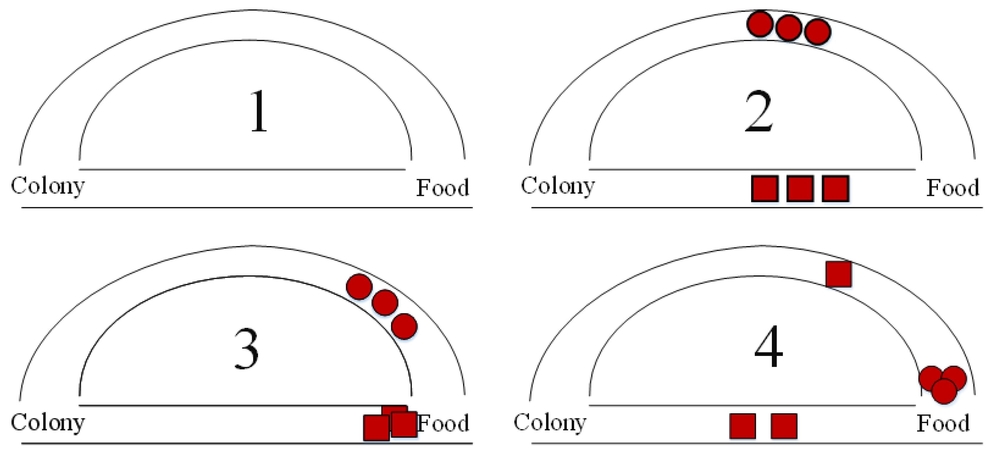
4. Ant Colony Optimization

Innovative algorithms are being created around the clock using new methods and tools to meet the demands of high-performance computing. Natural laws may serve as a source of inspiration for algorithms, leading to some very novel and exciting outcomes. It is in this category of algorithms that you’ll find evolutionary ones. These algorithms were developed to simulate some of the characteristics and behaviours seen in human evolution. In addition, the natural behaviour of animals might serve as a source of inspiration for such algorithmic design rather than only people. The primary goal of developing such approaches is to address issues that have not been adequately addressed by existing methods at an affordable cost. The Ant Colony Optimisation (ACO) method, developed by Marco Dorigo [21], takes its cues from the foraging activities of ant colonies. The behavior of ants in finding a way to find food was illustrated in Figure 5. The ant’s social nature means that it is better off as part of a colony than on its own. They communicate with one another using pheromones, touch, and sound. Organic chemical substances called pheromones are released by ants to encourage interaction between members of the same species. These are molecules that may influence the behaviour of other people by acting like hormones outside of the body of the person secreting them. Most ant colonies are ground-based, so it makes sense that pheromone trails would be laid out on the soil’s surface and tracked (smelled) by other ants. The core premise of ACO is based on the observation of ants as they leave their communal nests in search of food via the most direct route. At first, ants wander aimlessly about their nests in quest for food. This method of searching randomly provides many potential pathways to the food source from the nest. Now, ants take a bite out of the meal and bring it back with them, concentrating on the pheromones they will need along the way. These pheromone tests would determine the likelihood that subsequent ants would choose a certain route to the food source. This chance obviously depends on the pheromone’s concentration and its rate of evaporation. As the pheromone’s evaporation rate is also a determining factor, the length of each route may be calculated with relative ease.
For the sake of clarity, only two routes between the food source and the anthill have been shown in the preceding diagram. The steps can be broken down as follows:
First, the ants have returned to their nest. The atmosphere is devoid of any pheromones. (In algorithm development, the number of residual pheromones need not be ignored).
In Phase 2, the ants spread out over all possible routes with the same probability (half). The time it would take for the ants to travel the curved path to the food source is obviously longer.
Third, the ants who took the quickest route to the food source got there first. Clearly, they are back in the same situation they were in before, but this time, the pheromone trail down the shorter path that is already there makes it more likely that they will be chosen.
In the fourth phase, more ants use the shortcut to return, raising pheromone levels. In addition, as a result of evaporation, the concentration of pheromones along the longer journey decreases, making their selection less likely in later stages. As a result, it is more likely that the entire colony will adopt the shorter route over time. Hence, the optimum route is found.

4.1. Algorithmic Design

Based on the ants’ observed behaviour, we may now devise a suitable algorithm. For the sake of simplification, only a single food supply and a single ant colony with only two alternative routes have been studied. Weighted networks, with the ant colony and the food source as vertices (or nodes), the pathways as edges, and the pheromone levels as weights, can represent the entire scenario. Let the edges and vertices of the graph be V and E, respectively, and write the graph as G = (V, E). In our model, the vertices are the ant colony (Vs) and the food supply (Vd), the edges are E1 and E2, and the lengths of the edges are L1 and L2, respectively. For the vertices E1 and E2, we can assume the related pheromone values (which indicate their strength) to be R1 and R2, respectively. Hence, the initial probability of path selection (between E1 and E2) for each ant can be written as follows [21]:
P i = R i R 1 + R 2 i = 1 , 2
It stands to reason that if R1 > R2, then the odds of picking E1 are greater, and vice versa. Now, on the way back by the shortest path, say Ei, the pheromone value is updated for the associated route. Pheromone evaporation rates and route lengths are taken into account for this revision. This means that the upgrade can be implemented in stages.

4.2. In Accordance to Path Length

The below modification uses the model parameter “K,” with values of I equal to one and two [21]. In addition, the upgrade is path-dependent. The more concentrated the pheromone, the shorter the path.
R i R i + K L i  
According to the pheromone’s rate of dissipation [21].
R i ( 1 v ) R i
A parameter controls pheromone evaporation with a range of (0, 1) called v. Moreover, I = 1, 2, etc. All the ants have relocated to the source vertex vs. at each cycle (ant colony). Once step 1 is completed, ants travel from vs. to Vd (the food source). The second phase is when all the ants go back to their original trail and reinforce it. Due to the high power of this algorithm, it can be used to solve many different problems, including feature selection problems.

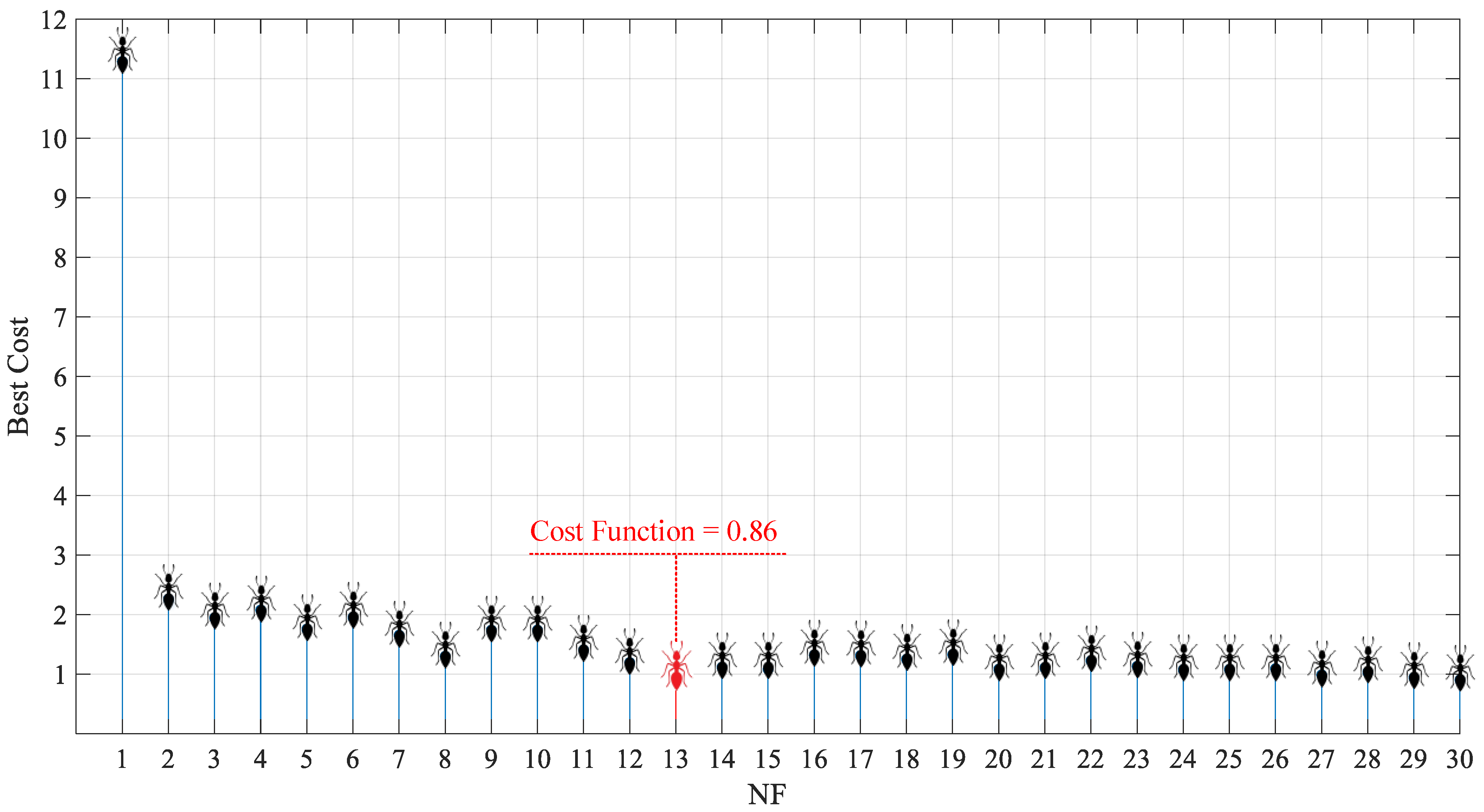
4.3. ACO-Based Feature Selection

In order to use this algorithm as a feature selection method, a cost function must first be defined. In this research, we designed an MLP neural network with one hidden layer and fifteen neurons in the hidden layer. The inputs of this network were initially selected randomly, and the neural network will be implemented to predict the target output (in this research, the target output was the scale thickness value). The mean square error (MSE) value between the target and neural network outputs will be defined as a cost function of the ACO. At first, one input was applied to this neural network. It was expected that in the first case, the value of the cost function would be high. In the next step, the number of inputs increases, and the ACO determines the appropriate combination of two features to reduce the cost function. In the same way, the number of selection entries increases, and the best combination of features is saved. The value of the cost function calculated by ACO according to the number of features (NF) can be seen in Figure 6. In this way, by comparing the cost function for the best combinations from one feature to thirty features, it was determined that the selection of thirteen features will have the lowest cost function with a value of 0.86. For this reason, the selection of thirteen features out of thirty features was introduced as the optimal mode. Table 1 shows the parameter values of the implemented ACO algorithm. In the beginning, taking into consideration the nature of the available data, the power of the available processor, and the load of calculations applied to the processor, these parameters were taken as an initial value, and their optimal value was selected in a repetitive train-test process.

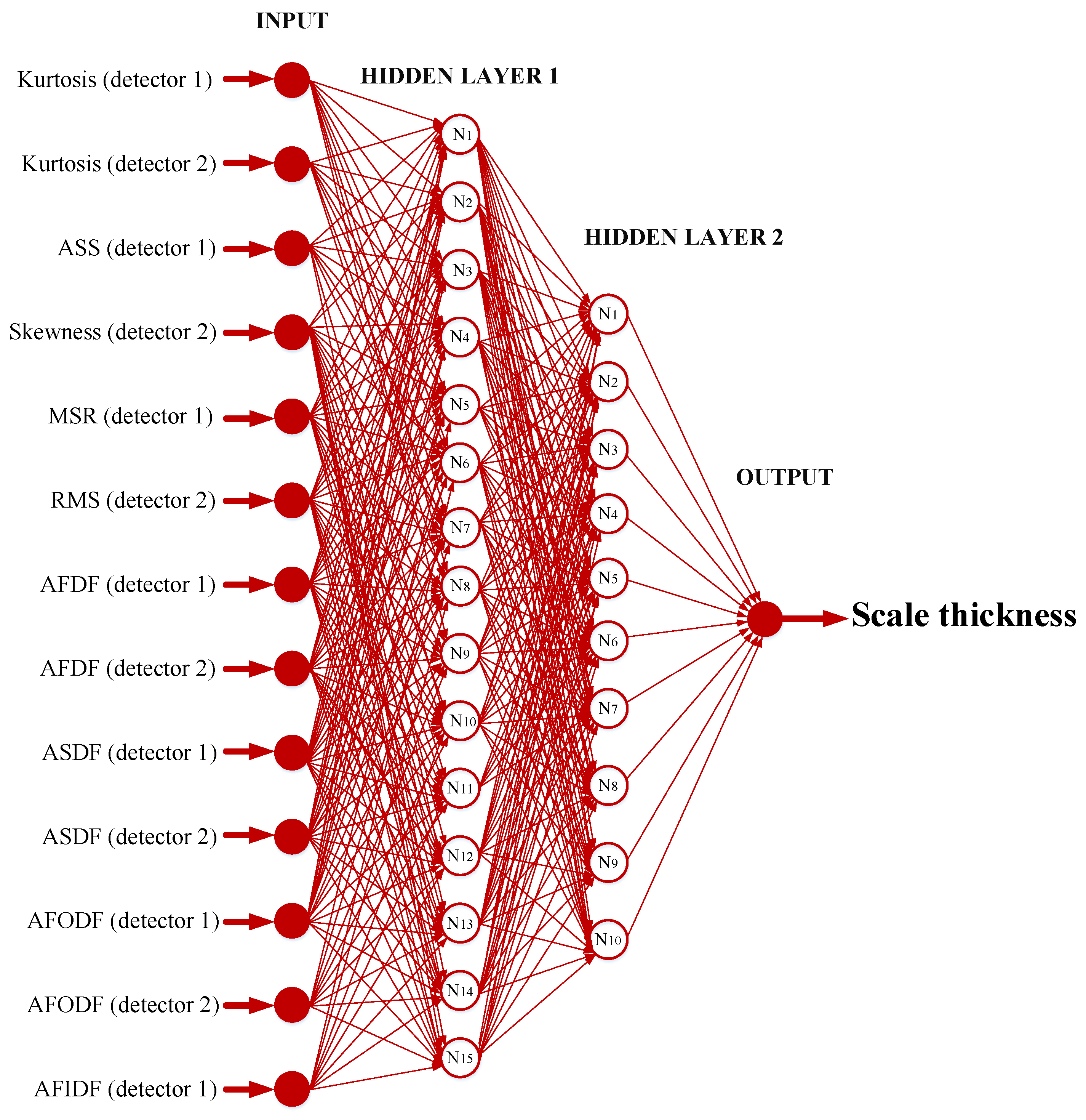
5. MLP Neural Network

These days, engineers are using all sorts of computational techniques to solve their research challenges [22,23,24,25,26,27,28,29,30,31,32,33,34,35,36,37,38,39,40,41,42,43,44,45,46,47,48,49,50,51]. The objective of this research was to determine the accuracy of an ANN method for estimating the thickness of scale deposits in oil pipes. Multi-layer perceptron (MLP) models, the most common kind of ANN, are used in a wide variety of contexts. Nonlinear functions and the various nonlinear decision surfaces are learned to be mapped to one another. These equations show how to get neurons to fire in the output layer: [52,53]:
n l = i = 1 u x i w i k + b k = 1 , 2 , , m
u j = f ( i = 1 u x i w i k + b ) k = 1 , 2 , , m
output = n = 1 j ( u n w n ) + b
In this equation, x represents the input parameters while w, b, and f represent the weighting factor, bias term, and activation function of the hidden layers, respectively. The number of neurons in each hidden layer is given by the index k, while the input is given by the letter i. In order to fine-tune the network’s weights, modern MLP networks are trained using the Levenberg-Marquardt approach, which makes use of the gradient and Hessian derivatives. The training phase employs 178 samples, the validation phase uses 37, and the testing phase employs 37. By segmenting the data into training, validation, and testing sets, the dangers of over- and under-training may be reduced. The bulk of the information used to teach a neural network consists of patterns and samples. The term “validation data” is used to describe the data used to evaluate the success of the training process. The test data are used in the last stage of training to fine-tune the neural network. If a neural network does well on this dataset, it will be robust enough to operate in the real world. Trained MLP-ANN models are used to predict the scale thickness in this paper. There were several iterations of ANN structures created and tuned until the error rate was minimised. Several configurations with varying numbers of neurons and activation functions were examined, including those with one, two, and three hidden layers. The ANN model was trained with the help of MATLAB 8.1.0.604 software.

6. Results

In this study, signals from two detectors were used to find fifteen time and frequency characteristics. There was a total of 30 features that could be used to figure out how thick the scale was inside the pipe. However, choosing the right feature to determine the parameter in question was a big challenge, which was solved with the help of ACO. ACO stated that using thirteen inputs has the lowest cost function. Thus, it was introduced as the optimal mode. After careful examination, it was found that the names of these thirteen entries are: 1-kurtosis first detector, 2-kurtosis second detector, 3-ASS first detector, a 4-skewness second detector, 5-MSR first detector, 6-RMS second detector, 7-AFDF first detector, 8-AFDF second detector, 9-ASDF first detector, 10-ASDF second detector, 11-AFODF first detector, 12-AFODF second detector, and 13-AFIDF first detector. These features were introduced to the inputs of an MLP neural network to predict the target parameter. In a systematic method, networks with the number of one hidden layer to four hidden layers and with different numbers of neurons were examined, and it was found that a network with two hidden layers and a number of hidden neurons of respectively 15 and 10 can predict the thickness of the scale with a root mean square error (RMSE) of 0.017. The structure of the designed neural network is shown in Figure 7. The performance of neural networks is displayed graphically using different methods. Regression diagrams and fitting diagrams are two very common methods for this purpose. In the regression diagram, the desired output and the predicted output are shown as a line and a circle, respectively. The mentioned graphs for three categories of training, validation, and testing data can be seen in Figure 8. This research provided a very high level of accuracy in determining the thickness of the scale, which was due to the use of a powerful optimisation algorithm to determine the appropriate features. The comparison of the present study with previous studies is shown in Table 2.
As can be seen from this table, the lack of feature extraction from the signals received by the detectors was a big gap that caused the error of the proposed system to be very high in the research [54,55,56]. In these studies, different neural networks were investigated, but the lack of proper inputs to the neural networks decreased their accuracy. In their next research, the researchers investigated the time, frequency, and wavelet transform characteristics to determine the parameters of the oil field. However, it seemed that the lack of using a proper feature selection method to select the most effective features was the main fault of these studies. The use of the extracted characteristics as neural network inputs without monitoring and checking them caused the neural networks to not be successful in determining their target parameters with such high accuracy [5,6,57,58]. Recently, researchers investigated the PSO algorithm to introduce effective characteristics to determine the parameters of the oil field and were able to significantly increase the accuracy of the detection systems [59,60]. By comparing the error of the systems presented in research [59,60] with other research, we will understand the importance of using feature selection methods to increase the accuracy of detection systems. For this reason, we decided to test the performance of another feature selection method in order to increase the accuracy of the detection system. In this research, the performance of the feature selection method based on the ACO algorithm was investigated on time and frequency characteristics, and it was found that the use of this algorithm and the characteristics introduced by this algorithm could significantly improve the accuracy of previous research. This is considered a great achievement in the design of diagnostic systems in the oil field. Considering the importance of extracting and selecting features in determining the parameters of the oil field, it is strongly recommended to the researchers of this field to pay special attention to the investigation of other characteristics of the received signals and the examination of the extracted characteristics with other optimization methods. In addition, investigating the performance of other neural networks in this field can be a suitable topic for future research. The main limitation of the current research is the use of radiation sources in the structure of the detection system. Due to the negative effects of radiation on people’s bodies, it is necessary to use special clothes when working with these devices. On the other hand, it is very difficult to transport these devices due to the inability to turn off the source, and it requires special radiation-limiting devices. In this research, the performance of the feature selection method based on the ACO algorithm was investigated on time and frequency characteristics, and it was found that the use of this algorithm and the characteristics introduced by this algorithm could significantly improve the accuracy of previous research. This is considered a great achievement in the design of diagnostic systems in the oil field. Reducing the number of computations being applied to the system is one of the benefits of this study. Using the helpful features of the incoming signals to create neural networks reduces the number of computations. The following computer setup was used to do the computations necessary for feature extraction, feature selection, and the configuration of neural networks, and the processing time was less than three minutes. Processor: Intel(R) Core i7-10750H CPU, RAM: 16 GB, GPU: GeForce GTX 1650 ti. This system, which is implemented in the simulation space, can be designed and built in the operational space as well, and by using the features, the neural network and the methodology introduced in this research, the accuracy of diagnosis can be significantly increased.

7. Conclusions

This study introduces a quick, easy-to-use, and accurate method for measuring the thickness of the scale within oil pipelines. In this research, gamma-ray attenuation was used to develop an efficient method for detecting the scale thickness of homogeneously flowing three-phase condensates. The detection system, which consists of a dual-energy gamma generator and two NaI detectors placed on opposite sides of the pipe, is modelled using the MCNP algorithm. A three-phase fluid was modelled at various volumetric fractions while exploring different scale values. The change in the intensity of transmitted photons from the source in the collision with a pipe that has a scale layer with different thicknesses is an important parameter in the design of a high-precision scale detection system. The signals received by the detector have a very non-linear relationship with the change in the thickness of the scale layer, so it is very important to use the methods of signal processing, feature extraction and feature selection. The number of extracted features is high, and it will increase the volume of calculations applied to the system, therefore, in order to select the effective features, the technique based on the ACO algorithm was used. The data from each detector was analysed to derive 15 time and frequency characteristics that would be used as inputs to the ACO algorithm. The result of using a feature selection algorithm based on ACO showed that the use of 13 features with the names of kurtosis first detector, kurtosis second detector, ASS first detector, skewness second detector, MSR first detector, RMS second detector, AFDF first detector, AFDF second detector, ASDF first detector, ASDF second detector, AFODF first detector, AFODF second detector, and AFIDF first detector are enough to achieve high accuracy. The aforementioned features were used as inputs for an MLP neural network, which then produced the scale thickness in centimetres as an output. The RMSE for this neural network’s prediction of the scale thickness is less than 0.017. The effectiveness of the ACO algorithm in introducing acceptable inputs is a key factor in the high accuracy achieved in this study, which is in turn owed to the careful selection of characteristics to be applied to the inputs of the neural network.

Author Contributions

Conceptualization, A.M.M., J.W.G.G. and E.E.-Z.; methodology, V.P.T.I. and H.H.A.; software, V.P.T.I. and N.K.S.; validation, V.P.T.I., J.W.G.G. and N.K.S.; formal analysis, J.W.G.G. and N.K.S.; investigation, V.P.T.I. and E.E.-Z.; resources, J.W.G.G. and E.E.-Z.; data curation, J.K.B.; writing—original draft preparation, J.K.B. and N.K.S.; writing—review and editing, H.H.A. and E.E.-Z.; visualization, J.K.B. and H.H.A.; supervision, A.M.M. and H.H.A.; project administration, A.M.M.; funding acquisition, A.M.M. and E.E.-Z. All authors have read and agreed to the published version of the manuscript.

Funding

The authors extend their appreciation to the Deanship of Scientific Research at King Khalid University for funding this work through large group Research Project under grant number RGP2/39/44. We acknowledge support by the German Research Foundation Projekt-Nr. 512648189 and the Open Access Publication Fund of the Thueringer Universitaets- und Landesbibliothek Jena.

Data Availability Statement

The data presented in this study are available on request from the corresponding author.

Conflicts of Interest

The authors declare no conflict of interest.

References

  1. Nazemi, E.; Roshani, G.H.; Feghhi, S.A.H.; Setayeshi, S.; Zadeh, E.E.; Fatehi, A. Optimization of a method for identifying the flow regime and measuring void fraction in a broad beam gamma-ray attenuation technique. Int. J. Hydrog. Energy 2016, 41, 7438–7444. [Google Scholar] [CrossRef]
  2. Roshani, M.; Phan, G.; Roshani, G.H.; Hanus, R.; Nazemi, B.; Corniani, E.; Nazemi, E. Combination of X-ray tube and GMDH neural network as a nondestructive and potential technique for measuring characteristics of gas-oil–water three phase flows. Measurement 2021, 168, 108427. [Google Scholar] [CrossRef]
  3. Roshani, G.H.; Nazemi, E.; Feghhi, S.A.H. Investigation of using 60Co source and one detector for determining the flow regime and void fraction in gas–liquid two-phase flows. Flow Meas. Instrum. 2016, 50, 73–79. [Google Scholar] [CrossRef]
  4. Roshani, G.H.; Karami, A.; Nazemi, E. An intelligent integrated approach of Jaya optimization algorithm and neuro-fuzzy network to model the stratified three-phase flow of gas–oil–water. Comput. Appl. Math. 2019, 38, 5. [Google Scholar] [CrossRef]
  5. Sattari, M.A.; Roshani, G.H.; Hanus, R.; Nazemi, E. Applicability of time-domain feature extraction methods and artificial intelligence in two-phase flow meters based on gamma-ray absorption technique. Measurement 2021, 168, 108474. [Google Scholar] [CrossRef]
  6. Sattari, M.A.; Roshani, G.H.; Hanus, R. Improving the structure of two-phase flow meter using feature extraction and GMDH neural network. Radiat. Phys. Chem. 2020, 171, 108725. [Google Scholar] [CrossRef]
  7. Alamoudi, M.; Sattari, M.A.; Balubaid, M.; Eftekhari-Zadeh, E.; Nazemi, E.; Taylan, O.; Kalmoun, E.M. Application of Gamma Attenuation Technique and Artificial Intelligence to Detect Scale Thickness in Pipelines in Which Two-Phase Flows with Different Flow Regimes and Void Fractions Exist. Symmetry 2021, 13, 1198. [Google Scholar] [CrossRef]
  8. Taylan, O.; Abusurrah, M.; Amiri, S.; Nazemi, E.; Eftekhari-Zadeh, E.; Roshani, G.H. Proposing an Intelligent Dual-Energy Radiation-Based System for Metering Scale Layer Thickness in Oil Pipelines Containing an Annular Regime of Three-Phase Flow. Mathematics 2021, 9, 2391. [Google Scholar] [CrossRef]
  9. Basahel, A.; Sattari, M.A.; Taylan, O.; Nazemi, E. Application of Feature Extraction and Artificial Intelligence Techniques for Increasing the Accuracy of X-ray Radiation Based Two Phase Flow Meter. Mathematics 2021, 9, 1227. [Google Scholar] [CrossRef]
  10. Taylan, O.; Sattari, M.A.; Elhachfi Essoussi, I.; Nazemi, E. Frequency Domain Feature Extraction Investigation to Increase the Accuracy of an Intelligent Nondestructive System for Volume Fraction and Regime Determination of Gas-Water-Oil Three-Phase Flows. Mathematics 2021, 9, 2091. [Google Scholar] [CrossRef]
  11. Roshani, G.H.; Ali PJ, M.; Mohammed, S.; Hanus, R.; Abdulkareem, L.; Alanezi, A.A.; Kalmoun, E.M. Simulation Study of Utilizing X-ray Tube in Monitoring Systems of Liquid Petroleum Products. Processes 2021, 9, 828. [Google Scholar] [CrossRef]
  12. Balubaid, M.; Sattari, M.A.; Taylan, O.; Bakhsh, A.A.; Nazemi, E. Applications of Discrete Wavelet Transform for Feature Extraction to Increase the Accuracy of Monitoring Systems of Liquid Petroleum Products. Mathematics 2021, 9, 3215. [Google Scholar] [CrossRef]
  13. Akyol, S.; Alatas, B. Plant intelligence based metaheuristic optimization algorithms. Artif. Intell. Rev. 2017, 47, 417–462. [Google Scholar] [CrossRef]
  14. Alatas, B.; Bingol, H. Comparative Assessment of Light-Based Intelligent Search and Optimization Algorithms. Light Eng. 2020, 28. [Google Scholar] [CrossRef]
  15. Hosseini, S.; Taylan, O.; Abusurrah, M.; Akilan, T.; Nazemi, E.; Eftekhari-Zadeh, E.; Roshani, G.H. Application of Wavelet Feature Extraction and Artificial Neural Networks for Improving the Performance of Gas–Liquid Two-Phase Flow Meters Used in Oil and Petrochemical Industries. Polymers 2021, 13, 3647. [Google Scholar] [CrossRef]
  16. Sattari, M.A.; Korani, N.; Hanus, R.; Roshani, G.H.; Nazemi, E. Improving the performance of gamma radiation based two phase flow meters using optimal time characteristics of the detector output signal extraction. J. Nucl. Sci. Technol. (JonSat) 2020, 41, 42–54. [Google Scholar]
  17. Iliyasu, A.M.; Mayet, A.M.; Hanus, R.; El-Latif, A.A.A.; Salama, A.S. Employing GMDH-Type Neural Network and Signal Frequency Feature Extraction Approaches for Detection of Scale Thickness inside Oil Pipelines. Energies 2022, 15, 4500. [Google Scholar] [CrossRef]
  18. Mayet, A.M.; Salama, A.S.; Alizadeh, S.M.; Nesic, S.; Guerrero, J.W.G.; Eftekhari-Zadeh, E.; Nazemi, E.; Iliyasu, A.M. Applying Data Mining and Artificial Intelligence Techniques for High Precision Measuring of the Two-Phase Flow’s Characteristics Independent of the Pipe’s Scale Layer. Electronics 2022, 11, 459. [Google Scholar] [CrossRef]
  19. Pelowitz, D.B. MCNP-X TM User’s Manual, Version 2.5.0. LA-CP-05e0369; Los Alamos National Laboratory: Los Alamos, NM, USA, 2005. [Google Scholar]
  20. Nussbaumer, H.J. The fast Fourier transform. In Fast Fourier Transform and Convolution Algorithms; Springer: Berlin/Heidelberg, Germany, 1981; pp. 80–111. [Google Scholar]
  21. Dorigo, M.; Blum, C. Ant colony optimization theory: A survey. Theor. Comput. Sci. 2005, 344, 243–278. [Google Scholar] [CrossRef]
  22. Zych, M.; Hanus, R.; Wilk, B.; Petryka, L.; Świsulski, D. Comparison of noise reduction methods in radiometric correlation measurements of two-phase liquid-gas flows. Measurement 2018, 129, 288–295. [Google Scholar] [CrossRef]
  23. Golijanek-Jędrzejczyk, A.; Mrowiec, A.; Hanus, R.; Zych, M.; Świsulski, D.U. Uncertainty of mass flow measurement using centric and eccentric orifice for Reynolds number in the range 10,000 ≤ Re ≤ 20,000. Measurement 2020, 160, 07851. [Google Scholar] [CrossRef]
  24. Mayet, A.; Hussain, M. Amorphous WNx Metal For Accelerometers and Gyroscope. In Proceedings of the MRS Fall Meeting, Boston, MA, USA, 30 November–5 December 2014. [Google Scholar]
  25. Mayet, A.; Hussain, A.; Hussain, M. Three-terminal nanoelectromechanical switch based on tungsten nitride—An amor-phous metallic material. Nanotechnology 2016, 27, 035202. [Google Scholar] [CrossRef] [PubMed]
  26. Shukla, N.K.; Mayet, A.M.; Vats, A.; Aggarwal, M.; Raja, R.K.; Verma, R.; Muqeet, M.A. High speed integrated RF–VLC data communication system: Performance constraints and capacity considerations. Phys. Commun. 2022, 50, 101492. [Google Scholar] [CrossRef]
  27. Mayet, A.; Smith, C.E.; Hussain, M.M. Energy reversible switching from amorphous metal based nanoelectromechanical switch. In Proceedings of the 13th IEEE International onference on Nanotechnology (IEEE-NANO 2013), Beijing, China, 5–8 August 2013; pp. 366–369. [Google Scholar]
  28. Artyukhov, A.V.; Isaev, A.A.; Drozdov, A.N.; Gorbyleva, Y.A.; Nurgalieva, K.S. The rod string loads variation during short-term annular gas extraction. Energies 2022, 15, 5045. [Google Scholar] [CrossRef]
  29. Isaev, A.A.; Aliev MM, O.; Drozdov, A.N.; Gorbyleva, Y.A.; Nurgalieva, K.S. Improving the efficiency of curved wells’ operation by means of progressive cavity pumps. Energies 2022, 15, 4259. [Google Scholar] [CrossRef]
  30. Alanazi, A.K.; Alizadeh, S.M.; Nurgalieva, K.S.; Guerrero, J.W.G.; Abo-Dief, H.M.; Eftekhari-Zadeh, E.; Nazemi, E.; Narozhnyy, I.M. Optimization of x-ray tube voltage to improve the precision of two phase flow meters used in petroleum industry. Sustainability 2021, 13, 13622. [Google Scholar] [CrossRef]
  31. Mayet, A.M.; Alizadeh, S.M.; Nurgalieva, K.S.; Hanus, R.; Nazemi, E.; Narozhnyy, I.M. Extraction of Time-Domain Charac-teristics and Selection of Effective Features Using Correlation Analysis to Increase the Accuracy of Petroleum Fluid Monitor-ing Systems. Energies 2022, 15, 1986. [Google Scholar] [CrossRef]
  32. Lalbakhsh, A.; Mohamadpour, G.; Roshani, S.; Ami, M.; Roshani, S.; Sayem, A.S.; Alibakhshikenari, M.; Koziel, S. Design of a compact planar transmission line for miniaturized rat-race coupler with harmonics suppression. IEEE Access 2021, 9, 129207–129217. [Google Scholar] [CrossRef]
  33. Hookari, M.; Roshani, S.; Roshani, S. High-efficiency balanced power amplifier using miniaturized harmonics suppressed cou-pler. Int. J. RF Microw. Comput.-Aided Eng. 2020, 30, e22252. [Google Scholar] [CrossRef]
  34. Lotfi, S.; Roshani, S.; Roshani, S.; Gilan, M.S. Wilkinson power divider with band-pass filtering response and harmonics suppres-sion using open and short stubs. Frequenz 2020, 74, 169–176. [Google Scholar] [CrossRef]
  35. Jamshidi, M.; Siahkamari, H.; Roshani, S.; Roshani, S. A compact Gysel power divider design using U-shaped and T-shaped res-onators with harmonics suppression. Electromagnetics 2019, 39, 491–504. [Google Scholar] [CrossRef]
  36. Roshani, S.; Jamshidi, M.B.; Mohebi, F.; Roshani, S. Design and modeling of a compact power divider with squared resonators using artificial intelligence. Wirel. Pers. Commun. 2021, 117, 2085–2096. [Google Scholar] [CrossRef]
  37. Roshani, S.; Azizian, J.; Roshani, S.; Jamshidi, M.B.; Parandin, F. Design of a miniaturized branch line microstrip coupler with a simple structure using artificial neural network. Frequenz 2022, 76, 255–263. [Google Scholar] [CrossRef]
  38. Khaleghi, M.; Salimi, J.; Farhangi, V.; Moradi, M.J.; Karakouzian, M. Application of Artificial Neural Network to Predict Load Bearing Capacity and Stiffness of Perforated Masonry Walls. Civil Eng. 2021, 2, 48–67. [Google Scholar] [CrossRef]
  39. Ya, K.Z.; Goryachev, B.; Adigamov, A.; Nurgalieva, K.; Narozhnyy, I. Thermodynamics and electrochemistry of the interaction of sphalerite with iron (II)-bearing compounds in relation to flotation. Resources 2022, 11, 108. [Google Scholar] [CrossRef]
  40. Mayet, A.M.; Nurgalieva, K.S.; Al-Qahtani, A.A.; Narozhnyy, I.M.; Alhashim, H.H.; Nazemi, E.; Indrupskiy, I.M. Proposing a high-precision petroleum pipeline monitoring system for identifying the type and amount of oil products using extraction of frequency characteristics and a MLP neural network. Mathematics 2022, 10, 2916. [Google Scholar] [CrossRef]
  41. Alanazi, A.K.; Alizadeh, S.M.; Nurgalieva, K.S.; Nesic, S.; Guerrero, J.W.G.; Abo-Dief, H.M.; Eftekhari-Zadeh, E.; Nazemi, E.; Narozhnyy, I.M. Application of neural network and time-domain feature extraction techniques for determining volumetric percentages and the type of two phase flow regimes independent of scale layer thickness. Appl. Sci. 2022, 12, 1336. [Google Scholar] [CrossRef]
  42. Ahmad, M.; Alfayad, M.; Aftab, S.; Khan, M.A.; Fatima, A.; Shoaib, B.; Daoud, M.S.; Elmitwally, N.S. Data and Machine Learning Fusion Architecture for Cardiovascular Disease Prediction. Comput. Mater. Contin. 2021, 69, 2717–2731. [Google Scholar] [CrossRef]
  43. Daoud, M.S.; Aftab, S.; Ahmad, M.; Khan, M.A.; Iqbal, A.; Abbas, S.; Iqbal, M.; Ihnaini, B. Machine Learning Empowered Software Defect Prediction System. Intell. Autom. Soft Comput. 2021, 31, 1287–1300. [Google Scholar] [CrossRef]
  44. Daoud, M.S.; Ayesh, A.; Al-Fayoumi, M.; Hopgood, A.A. Location Prediction Based on a Sector Snapshot for Location-Based Services. J. Netw. Syst. Manag. 2014, 22, 23–49. [Google Scholar] [CrossRef]
  45. Shehab, M.; Abualigah, L.; Jarrah, M.I.; Alomari, O.A.; Daoud, M.S. (AIAM2019) Artificial Intelligence in Software Engineering and inverse: Review. Int. J. Comput. Integr. Manuf. 2020, 33, 1129–1144. [Google Scholar] [CrossRef]
  46. Hanus, R.; Zych, M.; Golijanek-Jędrzejczyk, A. Measurements of Dispersed Phase Velocity in Two-Phase Flows in Pipelines Using Gamma-Absorption Technique and Phase of the Cross-Spectral Density Function. Energies 2022, 15, 9526. [Google Scholar] [CrossRef]
  47. Hanus, R.; Zych, M.; Golijanek-Jędrzejczyk, A. Investigation of liquid–gas flow in a horizontal pipeline using gamma-ray technique and modified cross-correlation. Energies 2022, 15, 5848. [Google Scholar] [CrossRef]
  48. Golijanek-Jędrzejczyk, A.; Mrowiec, A.; Kleszcz, S.; Hanus, R.; Zych, M.; Jaszczur, M. A numerical and experimental analysis of multi-hole orifice in turbulent flow. Measurement 2022, 193, 110910. [Google Scholar] [CrossRef]
  49. Jedkare, E.; Shama, F.; Sattari, M.A. Compact Wilkinson power divider with multi-harmonics suppression. AEU-Int. J. Electron. Commun. 2020, 127, 153436. [Google Scholar] [CrossRef]
  50. Dabiri, H.; Farhangi, V.; Moradi, M.J.; Zadehmohamad, M.; Karakouzian, M. Applications of Decision Tree and Random Forest as Tree-Based Machine Learning Techniques for Analyzing the Ultimate Strain of Spliced and Non-Spliced Reinforce-ment Bars. Appl. Sci. 2022, 12, 4851. [Google Scholar] [CrossRef]
  51. Zych, M.; Petryka, L.; Kępński, J.; Hanus, R.; Bujak, T.; Puskarczyk, E. Radioisotope investigations of compound two-phase flows in an ope channel. Flow Meas. Instrum. 2014, 35, 11–15. [Google Scholar] [CrossRef]
  52. Taylor, J.G. Neural Networks and Their Applications; John Wiley & Sons Ltd.: Brighton, UK, 1996. [Google Scholar]
  53. Gallant, A.R.; White, H. On learning the derivatives of an unknown mapping with multilayer feedforward networks. Neural Netw. 1992, 5, e129–e138. [Google Scholar] [CrossRef]
  54. Iliyasu, A.M.; Bagaudinovna, D.K.; Salama, A.S.; Roshani, G.H.; Hirota, K. A Methodology for Analysis and Prediction of Volume Fraction of Two-Phase Flow Using Particle Swarm Optimization and Group Method of Data Handling Neural Network. Mathematics 2023, 11, 916. [Google Scholar] [CrossRef]
  55. Peyvandi, R.G.; Rad, S.Z.I. Application of artificial neural networks for the prediction of volume fraction using spectra of gamma rays backscattered by three-phase flows. Eur. Phys. J. Plus 2017, 132, 511. [Google Scholar] [CrossRef]
  56. Mayet, A.M.; Alizadeh, S.M.; Kakarash, Z.A.; Al-Qahtani, A.A.; Alanazi, A.K.; Alhashimi, H.H.; Eftekhari-Zadeh, E.; Nazemi, E. Introducing a precise system for determining volume percentages independent of scale thickness and type of flow regime. Mathematics 2022, 10, 1770. [Google Scholar] [CrossRef]
  57. Roshani, M.; Sattari, M.A.; Ali, P.J.; Roshani, G.H.; Nazemi, B.; Corniani, E.; Nazemi, E. Application of GMDH neural network technique to improve measuring precision of a simplified photon attenuation based two-phase flowmeter. Flow Meas. Instrum. 2020, 75, 101804. [Google Scholar] [CrossRef]
  58. Roshani, G.H.; Nazemi, E.; Feghhi, S.A.; Setayeshi, S. Flow regime identification and void fraction prediction in two-phase flows based on gamma ray attenuation. Measurement 2015, 62, 25–32. [Google Scholar] [CrossRef]
  59. Hosseini, S.; Roshani, G.; Setayeshi, S. Precise gamma based two-phase flow meter using frequency feature extraction and only one detector. Flow Meas. Instrum. 2020, 72, 101693. [Google Scholar] [CrossRef]
  60. Chen, T.-C.; Alizadeh, S.M.; Albahar, M.A.; Thanoon, M.; Alammari, A.; Guerrero, J.W.G.; Nazemi, E.; Eftekhari-Zadeh, E. Introducing the Effective Features Using the Particle Swarm Optimization Algorithm to Increase Accuracy in Determining the Volume Percentages of Three-Phase Flows. Processes 2023, 11, 236. [Google Scholar] [CrossRef]
Figure 1. The general implementation process of the current research.
Processes 11 01621 g001
Figure 2. The architecture of the simulated detecting system.
Processes 11 01621 g002
Figure 3. Signals recorded by the first detector (a) 0 cm scale, (b) 0.5 cm scale, (c) 1 cm scale, (d) 1.5 cm scale, (e) 2 cm scale, (f) 2.5 cm scale, and (g) 3 cm scale.
Processes 11 01621 g003aProcesses 11 01621 g003b
Figure 4. Signals recorded by the second detector (a) 0 cm scale, (b) 0.5 cm scale, (c) 1 cm scale, (d) 1.5 cm scale, (e) 2 cm scale, (f) 2.5 cm scale, and (g) 3 cm scale.
Processes 11 01621 g004aProcesses 11 01621 g004b
Figure 5. The behavior of ants in finding a way to find food.
Processes 11 01621 g005
Figure 6. The value of the cost function calculated by ACO according to the NF.
Processes 11 01621 g006
Figure 7. Trained MLP network architecture.
Processes 11 01621 g007
Figure 8. The fitting and regression diagrams for (a) training, (b) validation, and (c) test data.
Processes 11 01621 g008aProcesses 11 01621 g008b
Table 1. the parameters of the ACO algorithm.
Parameter Value
Number of selected features 1–30
Cost function of the best mode 0.86
Maximum Number of Iterations20
Number of Ants (Population Size)15
Initial Pheromone1
Pheromone Exponential Weight1
Heuristic Exponential Weight1
Evaporation Rate0.05
Table 2. A comparison of the suggested detection system’s precision with earlier research.
Ref.Extracted FeaturesFeature Selection MethodType of Neural NetworkMaximum MSEMaximum RMSE
[5]Time featuresLack of feature selectionGMDH1.241.11
[6]Time featuresLack of feature selectionMLP0.210.46
[54]No feature extractionLack of feature selectionMLP2.561.6
[55]Lack of feature extractionLack of feature selectionGMDH7.342.71
[56]Frequency featuresLack of feature selectionMLP0.670.82
[57]Wavelet featuresLack of feature selectionGMDH0.190.44
[58]Full energy peak (transmission count), photon counts of Compton edge in the transmission detector and total count in the scattering detectorLack of feature selectionMLP1.081.04
[59]Frequency and wavelet featuresPSO-based feature selectionMLP0.130.36
[60]Time, wavelet, and frequency featuresPSO-based feature selectionGMDH0.090.30
[current study]Time and frequency featuresACO-based feature selectionMLP0.00020.017
Disclaimer/Publisher’s Note: The statements, opinions and data contained in all publications are solely those of the individual author(s) and contributor(s) and not of MDPI and/or the editor(s). MDPI and/or the editor(s) disclaim responsibility for any injury to people or property resulting from any ideas, methods, instructions or products referred to in the content.

