Artificial Neural Network Model for Temperature Prediction and Regulation during Molten Steel Transportation Process

Abstract

With the continuous optimization of the steel production process and the increasing emergence of smelting methods, it has become difficult to monitor and control the production process using the traditional steel management model. The regulation of steel smelting processes by means of machine learning has become a hot research topic in recent years. In this study, through the data mining and correlation analysis of the main equipment and processes involved in steel transfer, a network algorithm was optimized to solve the problems of standard back propagation (BP) networks, and a steel temperature forecasting model based on improved back propagation (BP) neural networks was established for basic oxygen furnace (BOF) steelmaking, ladle furnace (LF) refining, and Ruhrstahl–Heraeus (RH) refining. The main factors influencing steel temperature were selected through theoretical analysis and heat balance principles; the production data were analyzed; and the neural network was trained and tested using large amounts of field data to predict the end-point steel temperature of basic oxygen furnace (BOF) steelmaking, ladle furnace (LF) refining, and Ruhrstahl–Heraeus (RH) refining. The prediction model was applied to predict the degree of influence of different operating parameters on steel temperature. A comparison of the prediction results with the production data shows that the prediction system has good prediction accuracy, with a hit rate of over 90% for steel temperature deviations within 20 °C. Compared with the traditional steel temperature management model, the prediction system in this paper has higher management efficiency and a faster response time and is more practical and generalizable in the thermal management of steel.

1. Introduction

During ladle heat circulation, from the end of the last casting, the ladle goes through an empty stage, a baking stage, a steel discharge stage, a repacking stage, and a casting stage. The whole procedure is long, with many processes, long turnaround times, and large variations.

Basic oxygen furnace (BOF) steelmaking is of great importance; it is the main method of the steelmaking process in the thermal cycle of steel. In this process, hot metal and scrap are rapidly refined into liquid steel with the required carbon content by means of a supersonic oxygen injection from the top lance and through stirring from the bottom air outlet [1]. At the same time, melting agents such as lime and dolomite are added to the vessel for processing, and impurities are removed [2,3].

After the molten steel is produced from the converter, according to the smelting process objectives, it is also necessary to adjust the temperature and composition of the molten steel through external refining. Ladle furnace (LF) refining is one of the main methods of external refining, and with the development of production processes, Ruhrstahl–Heraeus (RH) refining has also received widespread attention in recent years as a way to improve refining efficiency. For different steel grades and working conditions, it is sometimes necessary to perform LF or RH refining, or both, on molten steel [4].

Ladle furnace (LF) refining requires stirring the molten steel in a low-oxygen atmosphere by blowing argon into the bottom of the furnace while heating the molten steel with graphite electrodes in order to regulate the composition and temperature of the molten steel. The temperature of the molten steel at the refining end point is one of the most important parameters in the steelmaking process, affecting steel quality, energy, and raw material consumption, as well as the probability of steel leakage accidents [5,6].

Ruhrstahl–Heraeus (RH) refining equipment is important in the steelmaking process and is used in almost all steel plants. It can perform various functions, such as vacuum degassing and decarbonization, composition and temperature homogenization, and temperature compensation and control. Ruhrstahl–Heraeus (RH) refining has become the main refining method for smelting due to its complete vacuum decarbonization and inclusion removal functions. The entire molten steel smelting reaction is carried out in a vacuum tank with a refractory lining. Equipment based on the principle of a bubble pump is used to draw molten steel through the degassing chamber and generate circular motion in order to remove gas in the vacuum chamber [7,8].

After the refining stage, the molten steel is transported to a continuous casting platform for casting. In order to ensure a stable process of continuous casting, stricter requirements are placed on the end temperature of the steel in the refining process: too high a steel temperature will reduce the lifespan of the furnace, increasing the heat load on the ladle and, thus, smelting costs, while too low a steel temperature will reduce the fluidity of the steel, easily blocking the water spout and increasing the rate of furnace return.

The smelting process of molten steel is a complex high-temperature physicochemical process involving uncertainty, strong coupling, large hysteresis, non-linearity, the inability to fully measure its state, and other features [9]. This process is difficult to accurately describe using the mechanistic model. The use of purely mechanistic models to forecast steel temperature requires the linearization of many non-linear factors affecting steel temperature and the stabilization of unstable factors; this simplifies a large number of conditions to create a model that differs significantly from the real condition, which means the prediction accuracy of the mechanistic model is not guaranteed.

Traditional production concepts and management are facing considerable challenges brought about by technological innovation. The recent advances in computational technologies and the ever-growing availability of data have enabled the development of sophisticated and efficient algorithms that can quickly process information [10].

Neural networks based on error backpropagation (BP) networks are highly capable and tolerant of faults in non-linear information, which allows them to process uncertain and ambiguous information in industrial production, analyze problems that are difficult to solve through modeling with mathematical planning models, control and predict complex, nonlinear industrial processes, and achieve arbitrary nonlinear mapping between inputs and outputs. Although the standard backpropagation (BP) algorithm has some problems, such as a low training rate, it can be optimized to solve these problems with good prediction accuracy and generalizability. Therefore, the use of machine learning models, such as artificial neural networks, has also attracted the attention of scholars in various fields [11,12] and these are widely used in the processes of predicting and controlling various nonlinear problems [13,14,15].

M.H. Sabzalian et al. proposed a lung cancer diagnosis system based on an improved bidirectional recurrent neural network and metaheuristic technique. The system was applied to the lung cancer dataset of the IQ- OTH/NCCD to properly authenticate the algorithm [16]. S. Altikat used multiple linear regression (MLR) artificial neural networks (ANN) and deep learning neural networks (DLNN) to model and study carbon dioxide flux from the soil to the atmosphere under greenhouse conditions [17]. I. V. Ofrikhter et al. proposed a neural network topology structure that predicts the mechanical properties of soil through physical parameters. Based on comparative results, the practicality of artificial neural networks in the field of geotechnical engineering was verified [18].

In the iron and steel industries, many metallurgical scholars have begun to focus their research on the intelligent control of metallurgical processes [19,20,21,22,23,24,25,26]. The artificial neural network model is widely used in the prediction of working conditions, such as head warpage [27], composition prediction [28], intermediate ladle steel flow characteristics [29], elemental content [30], data acquisition [31], the prediction of flame characteristics [32], and crack detection [33].

This paper establishes a big data analysis model describing the rhythm of the pro-duction process; it achieves this through the data mining and correlation analysis of the main equipment and processes involved in steel transfer that match the production process. Using a great data neural network, the model performs process index analysis with steel as the core, supports the operation of an intelligent scheduling platform for the production process, and analyzes the degree of influence of different operational factors on steel temperature using a prediction model, which can significantly increase productivity, provide response times for subsequent processes, and further regulate the material and energy balance in the production process. The mining of production data and the analysis and prediction of steel temperatures for the whole steel smelting process supplement the completeness of research in this area and solve the problems of complex working conditions, long cycle times, and difficult data collection, which make it difficult to analyze indicators under different stages of the whole process. The analysis of operational variables using large amounts of production data and predictive models is important for the further exploration of potential patterns in the steel smelting process.

2. Materials and Methods

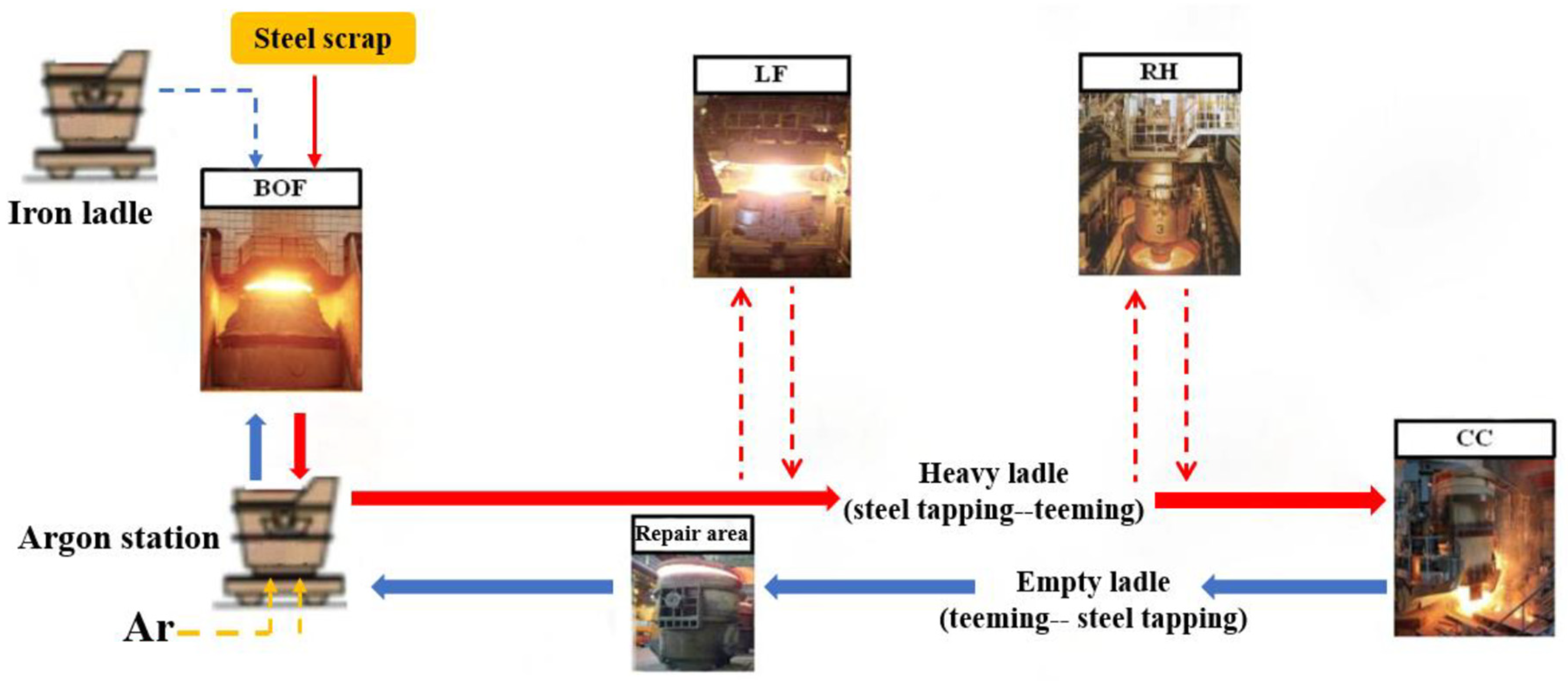
2.1. Factors Affecting the Temperature of Steel

The technological process of ladle operation in this study is shown in Figure 1. Based on the specific process flow and mechanism analysis, the key factors affecting the temperature of molten steel at the BOF, LF, and RH stages were selected.

2.1.1. Mechanism Analysis of BOF

The energy balance of the BOF is shown in Figure 2.

$$\Delta T_{BOF}=\Delta T_{melt}+\Delta T_{add}-\Delta T_{Ar}-\Delta T_{lining}$$

(1)

where $\Delta T_{BOF}$ is the value of the change in steel temperature during the steel discharge phase of the converter (°C); $\Delta T_{melt}$ is the temperature change caused by the addition of iron (°C); $\Delta T_{add}$ is the temperature change caused by the addition of materials (°C); $\Delta T_{Ar}$ is the temperature change caused by blowing argon and stirring (°C); and $\Delta T_{lining}$ is the temperature lost due to the furnace lining (°C).

The main task of this stage is to remove the carbon, silicon, manganese, phosphorus, sulfur, and oxygen contained in the iron to a certain extent under high-temperature oxidizing conditions and to raise the temperature to that of steel; this essentially involves a process of oxidizing the elements in the molten pool by releasing a large amount of heat.

The thermal effects resulting from the chemical reactions of the elements are shown in

Table 1. Thermal effects of chemical reactions [34].

Element	Reaction Formula	Reaction Heat (KJ/kg)
C	$\left[\mathrm{C}\right]+1/2{\mathrm{O}}_2=\mathrm{CO}$	10,950
C	$\left[\mathrm{C}\right]+{\mathrm{O}}_2={\mathrm{CO}}_2$	34,520
Si	$\left[\mathrm{Si}\right]+{\mathrm{O}}_2={\mathrm{SiO}}_2$	28,314
P	$2\left[\mathrm{P}\right]+5/2{\mathrm{O}}_2={\mathrm{P}}_2{\mathrm{O}}_5$	18,923
Mn	$\left[\mathrm{Mn}\right]+1/2{\mathrm{O}}_2=\mathrm{MnO}$	7020
Fe	$\left[\mathrm{Fe}\right]+1/2{\mathrm{O}}_2=\mathrm{FeO}$	5020
Fe	$\left[\mathrm{Fe}\right]+3/2{\mathrm{O}}_2={\mathrm{Fe}}_2{\mathrm{O}}_3$	6670
SiO2	${\mathrm{SiO}}_2+2\mathrm{CaO}=2\mathrm{CaO}·{\mathrm{SiO}}_2$	2070
P2O5	${\mathrm{P}}_2{\mathrm{O}}_5+4\mathrm{CaO}=4\mathrm{CaO}·{\mathrm{P}}_2{\mathrm{O}}_5$	5020

.

The main sources of heat in the converter steelmaking process are therefore the physical and chemical heat of the molten iron and the thermal effects of the addition of materials. The temperature losses during the discharge of steel from the converter are mainly caused by the radiation of the steel discharge jet, convective heat exchange with the outside air and the inner surface of the ladle, as well as argon agitation at the bottom of the ladle.

According to the principle of thermodynamics, the initial temperature of the steel is closely related to its heat, and the heat in the steel determines the internal energy of the steel, the entropy and size of the thermal radiation, the ability of the refractory materials to transfer heat, and other physical changes and chemical reactions generated by the heat; so, the initial temperature of the steel was selected as a variable to react to the thermal conductivity of the refractory materials, and temperature changes in the steel caused by argon stirring were determined by the duration of argon blowing. In addition, the initial amount of steel has an impact on the duration of steel output. However, not enough data were collected during the data collection process, so in this study, the melt pool level was used to reflect the amount of steel.

Based on the converter steelmaking and steel discharge processes, and through the above analysis, seven variables were ultimately selected as input variables for the neural network model: scrap input, iron water quantity, blowing duration, oxygen consumption, initial steel temperature, melt bath level, and argon-blowing duration.

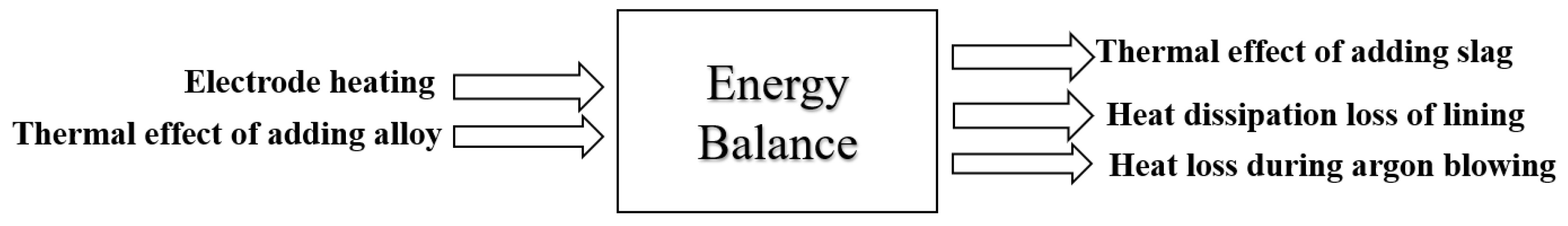
2.1.2. Mechanism Analysis of LF

The energy budget of the LF-refining process is shown in Figure 3.

$$\Delta T_{LF}=\Delta T_{arc}+\Delta T_{add}-\Delta T_{Ar}-\Delta T_{lining}$$

(2)

where $\Delta T_{LF}$ is the temperature variation of steel during LF refining (°C); $\Delta T_{arc}$ is the temperature change caused by arc heating (°C); $\Delta T_{add}$ is the temperature change caused by the thermal effect of adding alloys (°C); $\Delta T_{Ar}$ is the temperature loss caused by argon blowing and stirring (°C); and $\Delta T_{lining}$ is the temperature loss caused by ladle lining (°C).

In the LF-refining process, heat is mainly generated through the heating of the electricity supply and the thermal effect of the additives, and the loss of heat is mainly generated through heat dissipation from the ladle lining and through argon blowing and stirring.

The arc heating energy is directly determined by the arc power. The size of the arc power and the heating time can directly affect the heating efficiency of the steel temperature, which has a great impact on the steel temperature; thus, the arc power and the heating duration were selected as variables to reflect the degree of influence of arc heating on steel temperature.

In the refining process, materials need to be added to regulate the temperature and composition of the steel, including slag, alloys, etc. Slag entering the melt pool will have the effect of adsorbing inclusions, which is very beneficial to submerged arc heating and can improve the utilization of electrical energy. The alloy added to the molten steel will first be heated up and then melted; after this, it will be oxidized, depending on the alloy, to produce heat absorption and exothermic reactions, so the amount of material added has a direct impact on the temperature of the steel.

Argon blowing is an important part of the LF-refining process. Argon agitation accelerates the chemical reaction with the slag, facilitates the deoxidation and desulfurization of the steel, and also facilitates the removal of Al₂O₃-type inclusions and accelerates the uniformity of temperature and composition in the molten steel. Therefore, the argon-blowing duration and the amount of argon blowing affect changes in the temperature of the steel caused by argon stirring.

The heat of the steel is determined by its internal energy, entropy, the size of the heat radiation, and the ability of the resistant material to transfer heat, and in the steel smelting process, the steel and the work-resistant material are in direct contact with each other as boundary conditions; therefore, the initial temperature of the steel was chosen as the variable that reacts to the thermal conductivity of the resistant material.

Through an analysis of the temperature balance of the LF-refining process, the main factors influencing the temperature of the steel were identified to be electrical energy consumption, total heating time, argon blowing duration, argon-blowing consumption, initial steel temperature, and alloy addition.

2.1.3. Mechanism Analysis of RH

The energy budget of the RH furnace refining process is shown in Figure 4.

$$\Delta T_{RH}=\Delta T_{add}-\Delta T_{Ar}-\Delta T_{ladle}-\Delta T_{Vacuum}$$

(3)

where $\Delta T_{RH}$ is the temperature variation of steel during RH refining (°C); $\Delta T_{add}$ is the temperature change caused by the addition of Al (°C); $\Delta T_{Ar}$ is the temperature loss caused by argon blowing (°C); $\Delta T_{ladle}$ is the temperature loss caused by the ladle lining (°C); and $\Delta T_{Vacuum}$ is the temperature loss caused by the heat dissipation of refractory materials in the vacuum chambers (°C).

In the RH refining process, oxygen is one of the factors affecting the change in the temperature of steel. Generally, the following two effects are considered: the first is the effect of blowing oxygen dissolved in the steel into the vacuum chamber (which produces heat) on the temperature of the steel and the second is the effect of heat released in the deoxidation reaction of free oxygen in molten steel with carbon and aluminum on the temperature of molten steel.

The chemical reactions are shown in

Table 2. Thermal effects of chemical reactions [35].

Element	Reaction Formula	Reaction Heat (KJ/kg)
Decarbonization	$\left[\mathrm{C}\right]+\left[\mathrm{O}\right]=\mathrm{CO}$	−22.202
	$\mathrm{CO}+\left[\mathrm{O}\right]={\mathrm{CO}}_2$	−282.544
Aluminum oxide reaction	$\mathrm{Al}\left(\mathrm{s}\right)=\mathrm{Al}\left(\mathrm{l}\right)$	10.71
	$2\left[\mathrm{Al}\right]+3\left[\mathrm{O}\right]=\left({\mathrm{Al}}_2{\mathrm{O}}_3\right)$	−1205.12

:

It can be seen that both decarburization reactions and aluminum oxide reactions are directly related to oxygen content, and the heat released by the dissolved oxygen blown into the molten steel to form free oxygen is one of the factors that affect the temperature of the molten steel. Therefore, the amount of oxygen blown was selected as one of the variables that affect the temperature of the molten steel.

The effects of adding Al to the temperature of the steel manifest in two main ways. The heat caused by the reaction in this process is shown in Table 2.

The first effect involves heat absorption during the melting of solid aluminum:

$$Q_{Al}=\frac{m_{Al}·\Delta H_{Al}}{M_{Al}}$$

(4)

where $m_{Al}$ is the amount of Al added (kg) and $M_{Al}$ is the molar mass of Al ($M_{Al}=$ 27$\mathrm{g}/\mathrm{mol}$).

The second effect is that heat is given off by the reaction of the aluminum in the steel with free oxygen:

$$Q_{Al-O}=\frac{m_{Al}·\Delta H_{Al-O}}{2·M_{Al}}$$

(5)

$$\Delta T_{Al-O}=\frac{Q_{Al-O}-Q_{Al}}{m_s·c_p}$$

(6)

where $m_s$ is the amount of steel (kg); $c_p$ is the specific heat of the steel ($c_p=750\mathrm{J}/\mathrm{Kg}·K)$; and $\Delta T_{Al-O}$ is the value of the steel temperature change (°C).

Assuming the amount of steel is 180 t, the calculation shows that $\Delta T_{Al-O}=0.16·m_{Al}$. Each kilogram of Al added raises the temperature of the steel by 0.16 °C. In the production process, it is generally necessary to add a large amount of Al to regulate the temperature of the steel, so it can be seen that the addition of Al has a considerable effect on the temperature of the steel. The change in the temperature of molten steel caused by the addition of Al is affected by the amount added.

During the RH-refining process, the heat dissipation of the ladle and the vacuum chamber lining is one of the most important factors affecting the change in the temperature of molten steel. In the previous analysis, the initial temperature of molten steel was selected as an important factor affecting the change in the temperature of molten steel. In addition, the length of refining time seriously affects the change in the temperature of molten steel and can also reflect the temperature and state of the molten steel, ladle, vacuum chamber, and refractory materials. Therefore, RH-refining time is also an important factor affecting the change in the temperature of steel. In addition, the lowest vacuum degree was selected as a factor reflecting the state of the vacuum chamber during the refining process.

Through the above analysis, six factors, including the initial temperature of the steel, the total amount of top-blown oxygen, the initial amount of steel, the minimum vacuum, the refining duration, and the alloy addition amount, were ultimately selected as input variables for the neural network model.

2.2. Data Preprocessing

2.2.1. Data Outlier Elimination

The production data of a steel plant within half a year were summarized and sorted. During this process, the data exported from a database may exhibit anomalies (e.g., due to missing or abnormal data), which may lead to problems such as the lower prediction accuracy of the model. Therefore, outliers should be handled before building the model.

To ensure the accuracy of data, the method of directly eliminating abnormal values was adopted. If a certain datapoint exceeded the high or low amplitude limit, or a certain group of data was missing, this group of data was considered to contain errors and was thus eliminated. Finally, after data preprocessing, a total of 1800 sets of actual production data were obtained for building the prediction model, including 1000 sets for the BOF, 400 sets for the LF, and 400 sets for RH.

The normal fluctuation ranges of the key factors selected for the three production stages (the BOF, the LF, and RH) are shown in

Table 3. Key data and scope.

Working Condition	Parameter	Minimum	Maximum
BOF	Scrap input (kg)	24,650	71,100
	Iron water quantity (kg)	123,300	204,700
	Blowing duration (s)	533	1377
	Oxygen consumption (Nm3)	29	12,375
	Initial steel temperature (°C)	1112	1798
	Melt bath level (cm)	845	970
	Argon-blowing duration (s)	845	2285
LF	Electrical energy consumption (KWH)	1088	38,963
	Total heating time (min)	2	85
	Argon blowing duration (min)	33	198
	Argon-blowing consumption (Nm3)	1	98
	Initial steel temperature (°C)	936	1756
	Alloy addition (kg)	184	8593
RH	Initial steel temperature (°C)	1536	1648
	Total amount of top-blown oxygen (Nm3)	8	599
	Initial amount of steel (kg)	198,649	264,279
	Minimum vacuum (Pa)	50	826
	Refining duration (s)	1571	9190
	Alloy addition amount (kg)	182	8698

.

2.2.2. Data Normalization

Due to the different dimensions of the input data of the network, the range of variation varies greatly. When data with significant differences in size are simultaneously applied to the input nodes of the neural network, this can lead to difficulties in adjusting the weights of the network connection weight matrix, affecting the convergence speed and accuracy of the entire network. Therefore, it is necessary to normalize the input data of the neural network and the values of the input and output data of the network into the interval [0, 1] through transformation processing.

The normalization function is:

$$y=\frac{x-x_{min}}{x_{max}-x_{min}}$$

(7)

where $y$ is the normalization result of the data; $x$ is actual value of the data; $x_{min}$ is the minimum value of the parameter; and $x_{max}$ is the maximum value of the parameter.

Due to the large amount of data, a group of data was selected from the BOF, LF, and RH databases for preprocessing.

The preprocessing results are shown in

Table 4. Data preprocessing.

Working Condition	Parameter	Value	Preprocessing Data
BOF	Scrap input (kg)	50,000	0.546
	Iron water quantity (kg)	150,600	0.335
	Blowing duration (s)	701	0.199
	Oxygen consumption (Nm3)	8638	0.697
	Initial steel temperature (°C)	1624	0.746
	Melt bath level (cm)	880	0.280
	Argon-blowing duration (s)	1499	0.454
LF	Electrical energy consumption (KWH)	9356	0.218
	Total heating time (min)	21	0.229
	Argon-blowing duration (min)	93	0.364
	Argon-blowing consumption (Nm3)	6	0.052
	Initial steel temperature (°C)	1588	0.795
	Alloy addition (kg)	2717	0.301
RH	Initial steel temperature (°C)	1594	0.518
	Total amount of top-blown oxygen (Nm3)	149	0.239
	Initial amount of steel (kg)	236,160	0.572
	Minimum vacuum (Pa)	83	0.043
	Refining duration (s)	6603	0.660
	Alloy addition amount (kg)	2555	0.279

.

The rest of the data were processed in the same way. After preprocessing, some of the data were used as training data to establish the model, and the rest were used to verify the accuracy of the model.

2.3. Algorithm Description

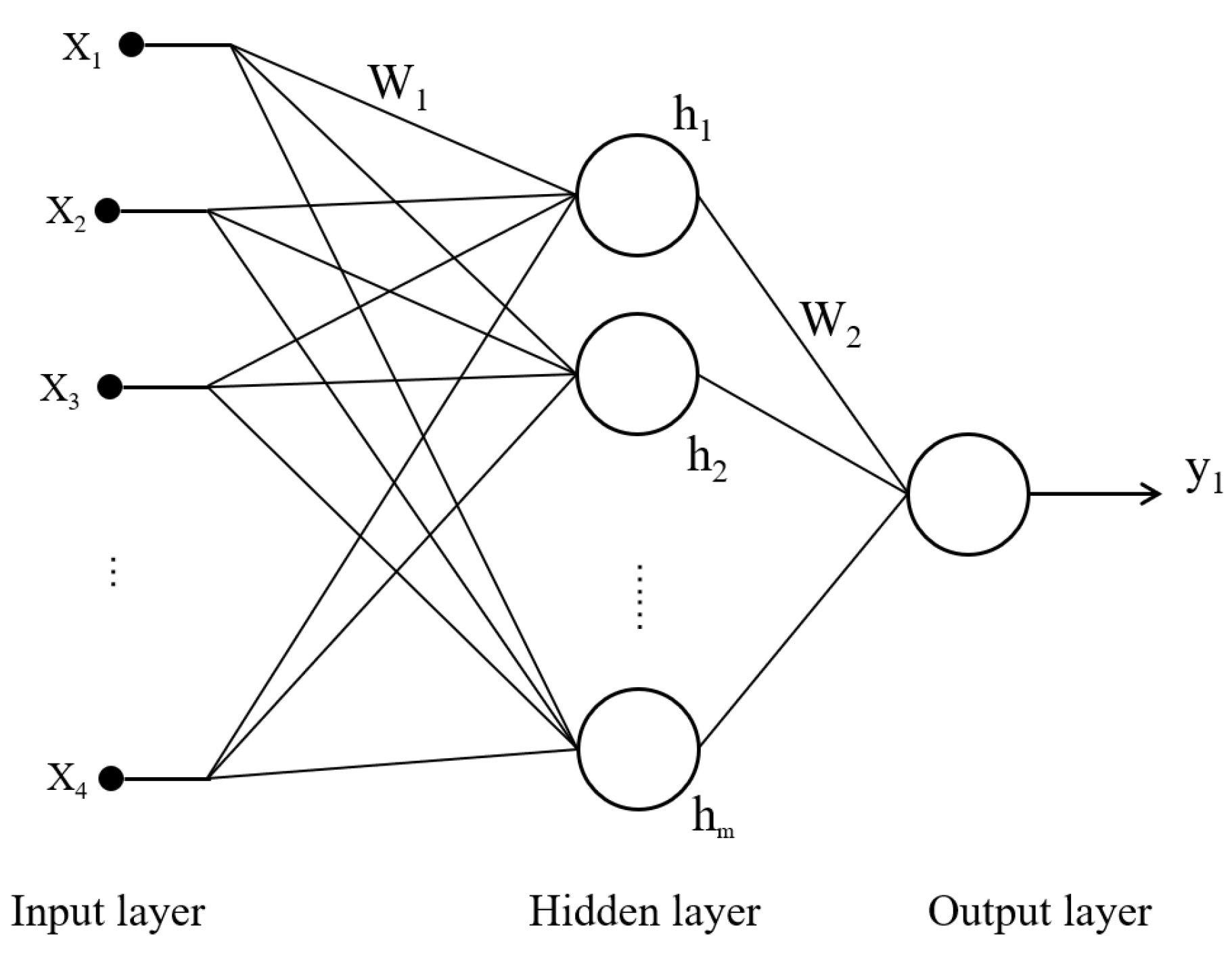
2.3.1. BP Neural Network

The BP neural network is a multi-layer feedforward network based on error backpropagation; it has a strong processing ability and fault tolerance for nonlinear information and can effectively predict the temperature of steel. The BP neural network model in this study uses a three-layer neural network, including an input layer, a hidden layer, and an output layer [36,37]. The input layer comprises the factors selected in the previous section that affect the steel temperature, and the output layer comprises the terminal steel temperature under corresponding working conditions. The neural network structure is shown in Figure 5.

2.3.2. Optimization of Network Algorithms

The standard BP algorithm has strong processing ability and fault tolerance for nonlinear information and can achieve arbitrary nonlinear mapping between the input and the output. However, it also has some disadvantages: for example, it has a low training rate; it can easily become trapped in the local minimum and fail to obtain global optimization; it has too many training times, making its learning efficiency low; and it has slow convergence speed.

In response to these problems, a momentum gradient descent backpropagation algorithm was used to optimize the neural network. This algorithm is based on the previous correction results and aims to affect the current correction amount. When the current correction amount is too large, a momentum factor is introduced to reduce the current correction amount, thereby reducing the effect of oscillation. When the current correction amount is too small, a momentum term is introduced to increase the current correction amount, thereby accelerating the correction.

The weight expression after introducing the momentum term is:

$$\Delta \omega \left(t\right)=\eta \delta X+\alpha \Delta \omega \left(t-1\right)$$

(8)

where $\omega$ is the weight matrix; $\eta$ is the learning rate; X is the input vector of this layer; and $\alpha$ is the momentum coefficient, located in the (0, 1) range.

When updating the weights and thresholds, not only was the current gradient direction considered but so was the gradient direction in the previous moment, which reduced the sensitivity of the network’s performance to parameter adjustment, effectively suppressed local minima, and introduced momentum terms. This ensured the stability of the algorithm while accelerating its convergence speed, resulting in a shorter learning time.

After verification, the learning rate of the BOF prediction model in this model was 0.2, and the momentum factor was 0.9; the momentum factor of the LF prediction model was 0.95 and the learning rate was 0.2; and the momentum factor of the RH prediction model was 0.9 and the learning rate was 0.15.

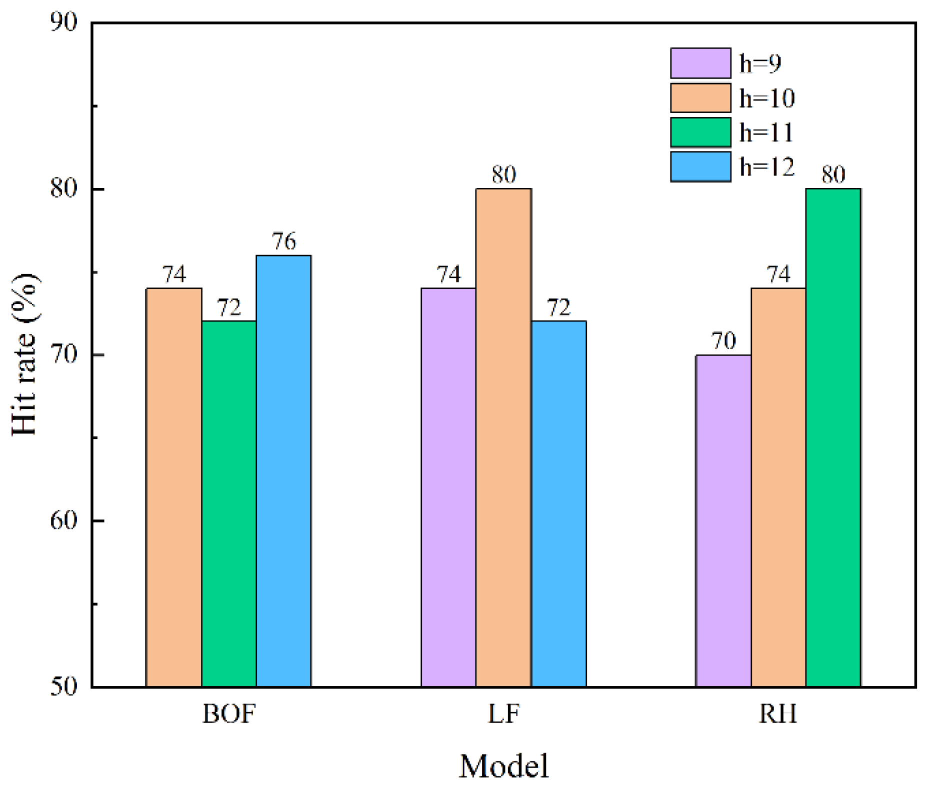
2.3.3. Selection of Hidden Layer Node Number

The selection of hidden layer nodes generally depends on the number of samples, the level of sample noise, and the complexity of the underlying laws in the samples. The number of hidden layer nodes needs to be determined through continuous training and comparison. In this study, the following empirical formula was used to initially determine the number of hidden layer nodes, and then to gradually increase or decrease the number of nodes in training based on the convergence effect:

$$h=\sqrt{n+m}+\sigma$$

(9)

where $h$ is the number of hidden layer nodes; $n$ is the number of input layer nodes; $m$ is the number of output layer nodes; and $\sigma$ is a constant between 1 and 10.

We selected the number of hidden layer nodes of the neural network model according to the formula; randomly selected 50 groups of samples from the databases of the BOF, LF, and RH models; and selected different hidden layer nodes to test the neural network model. The test results are shown in Figure 6.

The increase in the number of hidden layer nodes can enhance the ability to process signals and express patterns, but it can also lead to an increase in the learning time of the network. After testing, the BOF model took the number of hidden layer nodes to be 10, 11, and 12, respectively. The test results show that the hit rates for prediction deviations within ±10 °C were 74%, 72%, and 76%, respectively. The LF model took the number of hidden layer nodes to be 9, 10, 11, and 12, and the hit rates for prediction deviations within ±10 °C were 74%, 80%, 80%, and 72%, respectively. The RH model took the number of hidden layer nodes to be 9, 10, and 11, respectively. The test results show that the hit rates for prediction deviations within ±10 °C were 70%, 74%, and 80%, respectively.

According to the test results, the final number of hidden layer nodes selected for the BOF, LF, and RH models was 12, 10, and 11, respectively.

3. Results

With a trained neural network prediction model, the steel temperature at the transfer node and the impact of different operating parameters on the steel temperature can be predicted and checked in advance against the target value; when the predicted temperature differs significantly from the process target temperature, the steel temperature can be adjusted in advance by adjusting the process parameters, such as scrap input and iron input, to provide a response time for subsequent processes and reduce operating costs.

The model for predicting and adjusting the steel mixing temperature is shown in Figure 7.

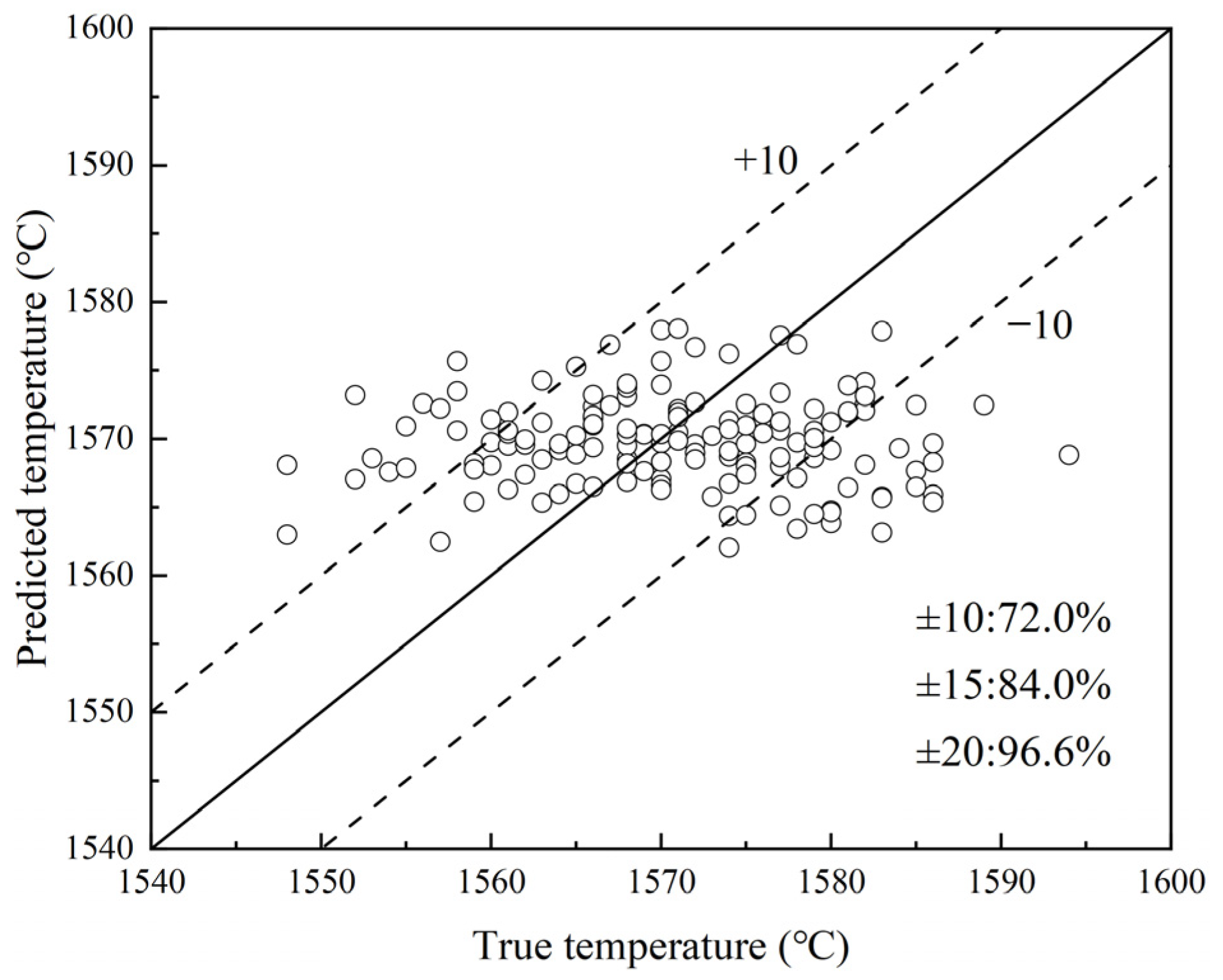
3.1. Sample Prediction

A neural network program was developed using C# language. The neural network model that was trained in the actual application process was applied directly. By collecting the production data of different conditions during the transfer process, a neural network prediction model was used to predict the end-point temperature of molten steel.

A random sample of 180, 150, and 150 groups was selected from the databases of the BOF, LF, and RH models, respectively, for end-point steel temperature prediction and compared with the actual results.

The prediction results for BOF end-point steel temperature are shown in Figure 8. By predicting the temperature of steel in the BOF stage, the prediction deviation within ±10 °C has a hit rate of 65%, that within ±15 °C has a hit rate of 83.3%, and that within ±20 °C has a hit rate of 94.4%.

The prediction results of the end-point steel temperature in LF refining are shown in Figure 9. The hit rate of the prediction deviation for LF refining within ±10 °C is 72%, the hit rate within ±15 °C is 84%, and the hit rate within ±20 °C reaches 96.6%.

The prediction results of the end-point steel temperature in RH refining are shown in Figure 10. The hit rate of prediction deviation for RH refining within ±10 °C is 74.7%, the hit rate within ±15 °C is 90.6%, and the hit rate within ±20 °C reaches 98%.

3.2. The Influence of Important Influencing Factors on the Temperature of Steel

After verification, the neural network model in this article had good accuracy. In order to further clarify the change rule of steel temperature and understand its degree of response to common operating factors, we conducted a specific analysis of the following factors that have a significant impact on steel temperature.

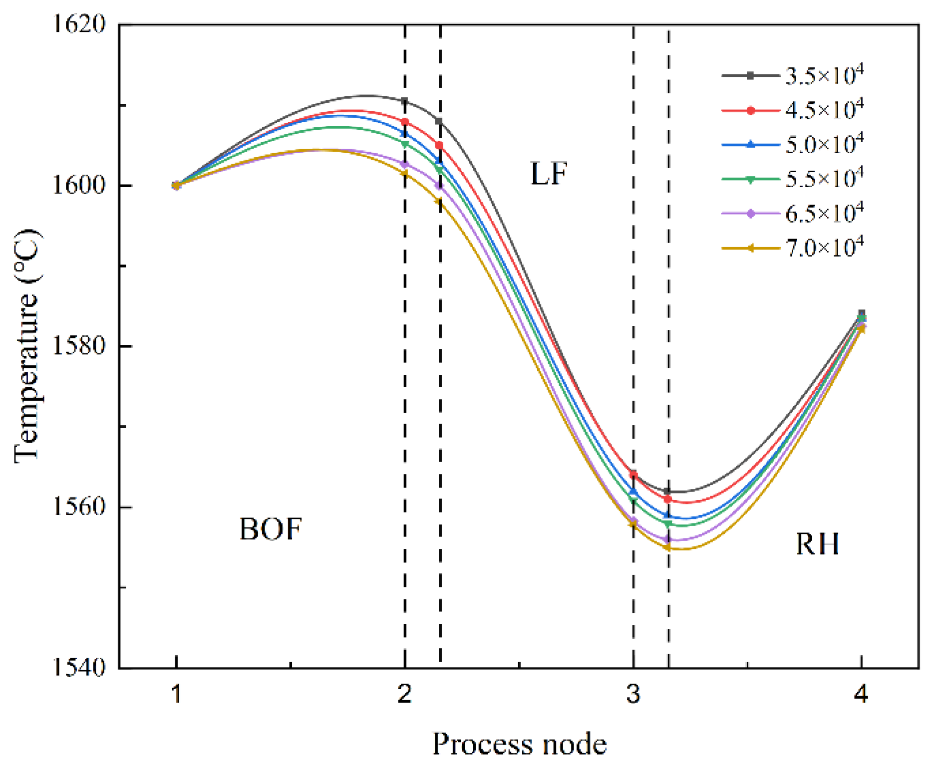
3.2.1. Effect of Scrap Input on Steel Temperature

The initial temperature of the steel was 1600 °C. After tapping from the converter, the steel in this furnace underwent LF refining–RH refining. During the converter steelmaking process, it is generally necessary to add scrap steel to adjust the temperature of the steel.

According to the verification results, upon adding different amounts of scrap (3.5 × 10⁴ kg~7.0 × 10⁴ kg) in stages, the final steel temperatures of the converter steel output were 1610 °C, 1607 °C, 1606 °C, 1605 °C, 1602 °C, and 1601 °C, respectively, and each additional 5 × 10³ kg of scrap input reduced the steel temperature by about 2~3 °C.

The effect of scrap input on steel temperature is shown in Figure 11.

3.2.2. Effect of Electric Energy Consumption on Steel Temperature

The initial temperature of the steel at the starting point of the LF stage was 1530 °C, and the steel in this furnace passed through the LF and RH refining stages in turn. In the LF refining process, arc heating is an important factor that affects the rise in the temperature of steel. Different electric energy consumption quantities were selected in order to predict the temperature of the steel.

According to the verification results, when the electric energy consumption values were 5000 KWh, 15,000 KWh, 25,000 KWh, and 35,000 KWh, the end-point steel temperatures of LF refining were 1566.98 °C, 1569.49 °C, 1572.16 °C, and 1575.10 °C, respectively. As the power consumption increased, every increase of 1 × 10⁴ KWh increased the temperature of steel by about 3 °C.

The influence of electric energy consumption on the temperature of steel is shown in Figure 12.

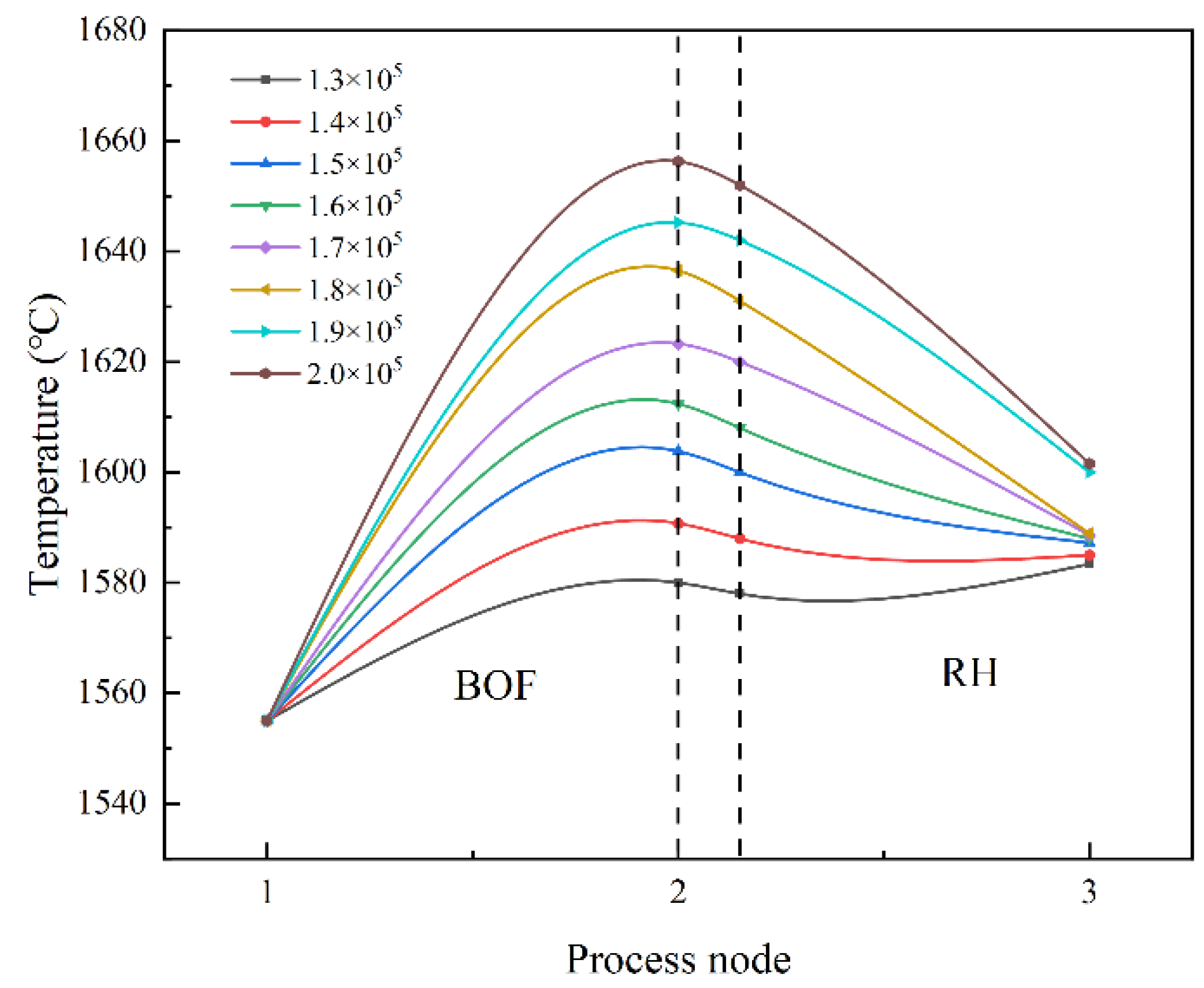
3.2.3. Effect of the Amount of Molten Iron Added on the Temperature of Steel

The influence of molten iron on the temperature of steel is mainly attributed to the physical heat of molten iron and the oxidation and exothermic heat of the chemical elements in molten iron. The initial temperature of the molten steel was 1555 °C. After calculation, we added different amounts of iron (1.3 × 10⁵ kg~2.0 × 10⁵ kg) to the converter and obtained steel temperatures of 1580.02 °C, 1590.74 °C, 1603.80 °C, 1612.37 °C, 1623.28 °C, 1636.54 °C, 1645.24 °C, and 1656.3 °C. The temperature of the steel increased by about 10 °C for every additional 1 × 10⁴ kg of iron input.

The effect of molten iron input on the temperature of steel is shown in Figure 13.

Upon verifying the neural network model, the results show that the hit rates for steel temperature forecast deviations within ±10 °C for BOF, LF, and RH refining are 65%, 72%, and 74.7%, respectively. The prediction accuracy within ±15 °C is above 80%, and the prediction accuracy within ±20 °C is above 90%. This indicates that the model has good prediction accuracy and can meet actual production requirements.

Every additional investment of 5 × 10³ kg scrap steel will reduce the end-point steel temperature of the converter by about 2–3 °C; as the power consumption increases, every increase of 1 × 10⁴ KWh will increase the temperature of the steel by about 3 °C; with every additional investment of 1 × 104 kg of molten iron, the temperature of the steel will increase by about 10 °C.

As shown in the above analysis, predicting the temperature of steel in advance can effectively standardize the objectives of the smelting process, optimize the production rhythm, and provide a response time for subsequent processes. In addition, the analysis of the impact of various scrap steel inputs and other factors on the temperature of steel could provide a reference for on-site production; this could be conducive to improving the material and energy balance of each product under the standardized process.

4. Discussion

This paper studies the temperature of steel at different process nodes in the process of steel transfer. By combining mechanism analysis and data analysis, an artificial neural network is optimized through the momentum gradient descent method. The temperature of steel at the transfer node and the related variables that affect the steel are predicted and analyzed. The accuracy of the model is verified via data validation from production practice to ensure the accuracy of the results.

Based on the mechanism analysis of the steel’s state at different transfer nodes of the BOF, the LF, and the RH, the pathways of temperature increase and decrease were identified and combined with production practice data, and the main variables affecting steel temperature were screened.

The production data were preprocessed. In order to ensure the accuracy of the data, a method of eliminating outliers was adopted to process missing and abnormal data, and the data were normalized in order to eliminate different production data that could affect the prediction results due to different dimensions and other factors.

In response to the low training efficiency of standard BP neural networks, a momentum gradient descent method was used to optimize the network algorithm. By comparing the prediction results of neural network models under different hidden layer node numbers, it was found that for the three temperature prediction models (BOF, LF, and RH), the prediction accuracy was higher when the numbers of hidden layer nodes were 12, 10, and 11, respectively.

The final prediction results show that among the three prediction models, the accuracy of the temperature deviation of steel at 20 °C reached over 90%, and the impact of factors such as scrap input on the temperature of steel was also accurately predicted. Therefore, the neural model has good prediction accuracy.

5. Conclusions

This article proposes a temperature prediction system for the molten steel transportation process based on artificial neural networks. The model studies the data of the thermal cycling process of molten steel, and analyzes and screens the process operating parameters, with molten steel as the core, through mechanism analysis and data analysis methods.

The production data were pre-processed prior to application, including the removal of abnormal data and data normalization, and validated against each other to achieve accurate predictions of steel temperature. The relevant operating parameters affecting steel temperature were analyzed via the prediction system to determine the impact of changes in the operating parameters on steel; the results of this analysis can be applied to the regulation of the steel temperature.

The research in this paper is based on the collection and collation of large amounts of production data, but due to the long cycle of the process, data collection was sometimes difficult; moreover, due to cost and safety considerations, the amount of data was insufficient, which, to some extent, affected the prediction results. For example, not enough data were collected regarding the amount of steel, so data for the melt pool level were used instead. In addition, the working conditions in the steel smelting process are complex and varied. Thus, in the future, the further collection and analysis of production data should be conducted under different working conditions, together with the practical application of the prediction system over a long period of time. In doing so, more revised data can be obtained so that the model can be applied to more situations, enabling researchers to determine the laws of steel smelting under different working conditions and further improve the accuracy and comprehensiveness of the prediction system.

References

1. Liu, G.Q.; Li, J.N.; Xu, D.; Zheng, B. Energy balance between multiple supersonic jets and molten bath in BOF steelmaking. Ironmak. Steelmak. 2022, 49, 726–736. [Google Scholar] [CrossRef]
2. Zhou, K.X.; Lin, W.H.; Sun, J.K.; Zhang, J.S.; Zhang, D.Z.; Feng, X.M.; Liu, Q. Prediction model of end-point phosphorus content for BOF based on monotone-constrained BP neural network. J. Iron. Steel Res. Int. 2022, 29, 751–760. [Google Scholar] [CrossRef]
3. Wang, Z.; Liu, Q.; Liu, H.T.; Wei, S.Z. A review of end-point carbon prediction for BOF steelmaking process. High Temp. Mater. Process. 2020, 39, 653–662. [Google Scholar] [CrossRef]
4. Guo, J.; Cheng, S.S.; Guo, H.J. Thermodynamics and Industrial Trial on Increasing the Carbon Content at the BOF Endpoint to Produce Ultra-Low Carbon IF Steel by BOF-RH-CSP Process. High Temp. Mater. Process. 2019, 38, 822–826. [Google Scholar] [CrossRef]
5. Yuan, F.; Xu, A.J.; Gu, M.Q. Development of an improved CBR model for predicting steel temperature in ladle furnace refining. Int. J. Miner. Metall. Mater. 2021, 28, 1321–1331. [Google Scholar] [CrossRef]
6. Shi, C.Y.; Guo, S.Y.; Wang, B.S.; Yin, X.X.; Sun, P.; Wang, Y.K.; Zhang, L.; Ma, Z.C. The Forcast of Slag Addition during the Ladle Furnace (LF) Refining Process Based on LWOA-TSVR. Metalurgija 2023, 62, 197–200. Available online: https://hrcak.srce.hr/290050 (accessed on 3 April 2023).
7. Feng, K.; Xu, A.J.; Wu, P.F.; He, D.F.; Wang, H.B. Case-based reasoning model based on attribute weights optimized by genetic algorithm for predicting end temperature of molten steel in RH. J. Iron. Steel Res. Int. 2019, 26, 585–592. [Google Scholar] [CrossRef]
8. Zhu, G.S.; Deng, X.X.; Ji, C.X. Effect of vacuum degree on inclusion removal in ultra-low carbon steel during RH refining process. Iron. Steel. 2022, 57, 99–105. [Google Scholar] [CrossRef]
9. Bi, C.B.; Zhang, Y.Z.; Shi, S.Y.; Guo, Y.X.; Huang, J. Prediction on temperature of hot metal on ironmaking and steelmaking interface based on GA-BP. J. Mater. Metall. 2021, 20, 17–22. [Google Scholar] [CrossRef]
10. Machado, E.; Pinto, T.; Guedes, V.; Morais, H. Electrical Load Demand Forecasting Using Feed-Forward Neural Networks. Energies 2021, 14, 7644. [Google Scholar] [CrossRef]
11. Hancock, J.T.; TKhoshgoftaar, M. Survey on categorical data for neural networks. J. Big Data 2020, 7, 993–1022. [Google Scholar] [CrossRef]
12. Mohammadazadeh, A.; Sabzalian, M.H.; Castillo, O.; Rathinasamy, S.; El-Sousy, F.F.M.; Mobayen, S. Neural Networks and Learning Algorithms in MATLAB; Springer: Berlin/Heidelberg, Germany, 2022. [Google Scholar] [CrossRef]
13. Duarte, I.C.; Almeida, G.M.; Cardoso, M. Heat-loss cycle prediction in steelmaking plants through artificial neural network. J. Oper. Res. Soc. 2022, 73, 326–337. [Google Scholar] [CrossRef]
14. Wang, L.; Ji, X.M.; Liu, J. Application of artificial intelligence in intelligent manufacturing in steel industry. Iron. Steel. 2021, 56, 1–8. [Google Scholar] [CrossRef]
15. Zhang, X.Q. Application of Artificial Neural Networks in Iron and Steel Materials Research. Metal. Mater. Metall. Eng. 2012, 40, 59–63. [Google Scholar] [CrossRef]
16. Sabzalian, M.H.; Kharajinezhadian, F.; Tajally, A.; Reihanisaransari, R.; Hamzah, A.A.; Bokov, D. New bidirectional recurrent neural network optimized by improved Ebola search optimization algorithm for lung cancer diagnosis. Biomed. Signal Process. Control. 2023, 84, 104965. [Google Scholar] [CrossRef]
17. Altikat, S. Prediction of CO2 emission from greenhouse to atmosphere with artificial neural networks and deep learning neural networks. Int. J. Environ. Sci. Technol. 2021, 18, 3169–3178. [Google Scholar] [CrossRef]
18. Ofrikhter, I.V.; Ponomaryov, A.B.; Zakharov, A.V.; Shenkman, R.I. Estimation of soil properties by an artificial neural network. Mag. Civ. Eng. 2022, 110, 11011. [Google Scholar] [CrossRef]
19. Akiyama, K.; Kang, I.; Kanno, T.; Uchida, N. Prediction of Residual Mg Contents in Ladle and Product after Graphite Spheroidizing Treatment by Using Artificial Neural Network: Technical Article. Mater. Trans. 2021, 62, 461–467. [Google Scholar] [CrossRef]
20. Wang, X.J.; You, M.S.; Mao, Z.Z.; Yuan, P. Tree-Structure Ensemble General Regression Neural Networks applied to predict the molten steel temperature in Ladle Furnace. Adv. Eng. Inf. 2016, 30, 368–375. [Google Scholar] [CrossRef]
21. He, F.; He, D.F.; Xu, A.J.; Wang, H.B.; Tian, N.Y. Hybrid Model of Molten Steel Temperature Prediction Based on Ladle Heat Status and Artificial Neural Network. J. Iron. Steel Res. Int. 2014, 21, 181–190. [Google Scholar] [CrossRef]
22. Liu, Z.; Cheng, S.S.; Liu, P.B. Prediction model of BOF end-point P and O contents based on PCA–GA–BP neural network. High Temp. Mater. Process. 2022, 41, 505. [Google Scholar] [CrossRef]
23. Smith, J.L. Advances in neural networks and potential for their application to steel metallurgy. Mater. Sci. Technol. 2020, 36, 1805–1819. [Google Scholar] [CrossRef]
24. Simion, C.P.; Verde, C.A.; Mironescu, A.A.; Anghel, F.G. Digitalization in Energy Production, Distribution, and Consumption: A Systematic Literature Review. Energies 2023, 16, 1960. [Google Scholar] [CrossRef]
25. Zeng, G.Q.; Wang, J.T.; Zhang, L.; Xie, X.Y.; Wang, X.F.; Chen, G.B. Multi-Domain Modeling and Analysis of Marine Steam Power System Based on Digital Twin. J. Mar. Sci. Eng. 2023, 11, 429. [Google Scholar] [CrossRef]
26. Wang, M.; Gao, C.; Ai, X.G.; Zhai, B.P.; Li, S.L. Whale Optimization End-point Control Model for 260 tons BOF Steelmaking. ISIJ Int. 2022, 62, 1684–1693. [Google Scholar] [CrossRef]
27. Huang, H.G.; Liu, Y.G.; Huang, H.L.; Chen, G.; Wang, X.D. Prediction and control for head warpage of hot-rolled slab based on machine vision detection and BP neural network. Chin. Metall. 2022, 32, 85–89, 96. [Google Scholar] [CrossRef]
28. Wen, H.; Zhu, S.X.; Han, F.; Zhu, Z.M.; Yu, H. Composition optimization and production practice of large angle steel for iron tower based on BP neural network. J. Iron. Steel Res. Int. 2022, 34, 95–100. [Google Scholar] [CrossRef]
29. Choi, B.; Lee, S.; You, D. Prediction of molten steel flow in a tundish with water model data using a generative neural network with different clip sizes. J. Mech. Sci. Technol. 2022, 36, 749–759. [Google Scholar] [CrossRef]
30. Xuan, M.T.; Li, J.J.; Wang, N.; Chen, M. Endpoint prediction of basic oxygen furnace steelmaking based on FOA-GRNN model. J. Mater. Metall. 2019, 18, 31–36, 57. [Google Scholar] [CrossRef]
31. Lee, J.; Lee, Y.C.; Kim, J.T. Migration from the traditional to the smart factory in the die-casting industry: Novel process data acquisition and fault detection based on artificial neural network. J. Mater. Process. Technol. 2021, 290, 116972. [Google Scholar] [CrossRef]
32. Chi, C.; Janiga, G.; Thevenin, D. On-the-fly artificial neural network for chemical kinetics in direct numerical simulations of premixed combustion. Combust. Flame. 2021, 226, 467–477. [Google Scholar] [CrossRef]
33. Cui, X.N.; Wang, Q.C.; Dai, J.P.; Xue, Y.J.; Duan, Y. Intelligent crack detection based on attention mechanism in convolution neural network. Adv. Struct. Eng. 2021, 24, 1859–1868. [Google Scholar] [CrossRef]
34. Gao, M. Basic Research on Scrap Melting Processes in Steelmaking Processes. Ph.D. Thesis, University of Science and Technology Beijing, Beijing, China, 2021. [Google Scholar] [CrossRef]
35. Wu, Y. Research on Temperature Prediction and Control Model for RH Vacuum Refining. Master’s Thesis, Wuhan University of Science and Technology, Wuhan, China, 2014. [Google Scholar] [CrossRef]
36. Maria, T.G.; Stefano, C.; Sudip, C.; Vincenza, C. Application of Artificial Neural Networks for Modelling and Control of Flux Decline in Cross-Flow Whey Ultrafiltration. Processes 2023, 11, 1287. [Google Scholar] [CrossRef]
37. Yagan, Y.E.; Vardar, K. Artificial neural networks controllers for three-phase neutral point clamped inverters. Eng. Sci. Technol. an Int. J. 2023, 41, 101390. [Google Scholar] [CrossRef]
Figure 1. Flow chart of the ladle operation process.
Processes 11 01629 g001
Figure 2. Energy balance of BOF.
Processes 11 01629 g002
Figure 3. Energy balance of LF refining.
Processes 11 01629 g003
Figure 4. Energy balance of RH refining.
Processes 11 01629 g004
Figure 5. Network structure.
Processes 11 01629 g005
Figure 6. Test results of neural network model.
Processes 11 01629 g006
Figure 7. Steel temperature prediction and regulation model.
Processes 11 01629 g007
Figure 8. Prediction Results of BOF.
Processes 11 01629 g008
Figure 9. Prediction results of LF refining.
Processes 11 01629 g009
Figure 10. Prediction results of RH refining.
Processes 11 01629 g010
Figure 11. Effect of scrap input on molten steel temperature.
Processes 11 01629 g011
Figure 12. Effect of electric energy consumption on molten steel temperature.
Processes 11 01629 g012
Figure 13. Effect of molten iron input on molten steel temperature.
Processes 11 01629 g013