5.1. Optimization Schemes and Parameters
In this paper, the improved IEEE33 node is selected to analyze and verify the SOP and ESS access planning in the distribution network. The improved voltage level of the IEEE33 node is 12.66 KV, the total active load is 3175 KW, and the fault lines are between nodes 6 and 7 and between nodes 15 and 16. The system-structure diagram of the improved IEEE33 nodes is shown in
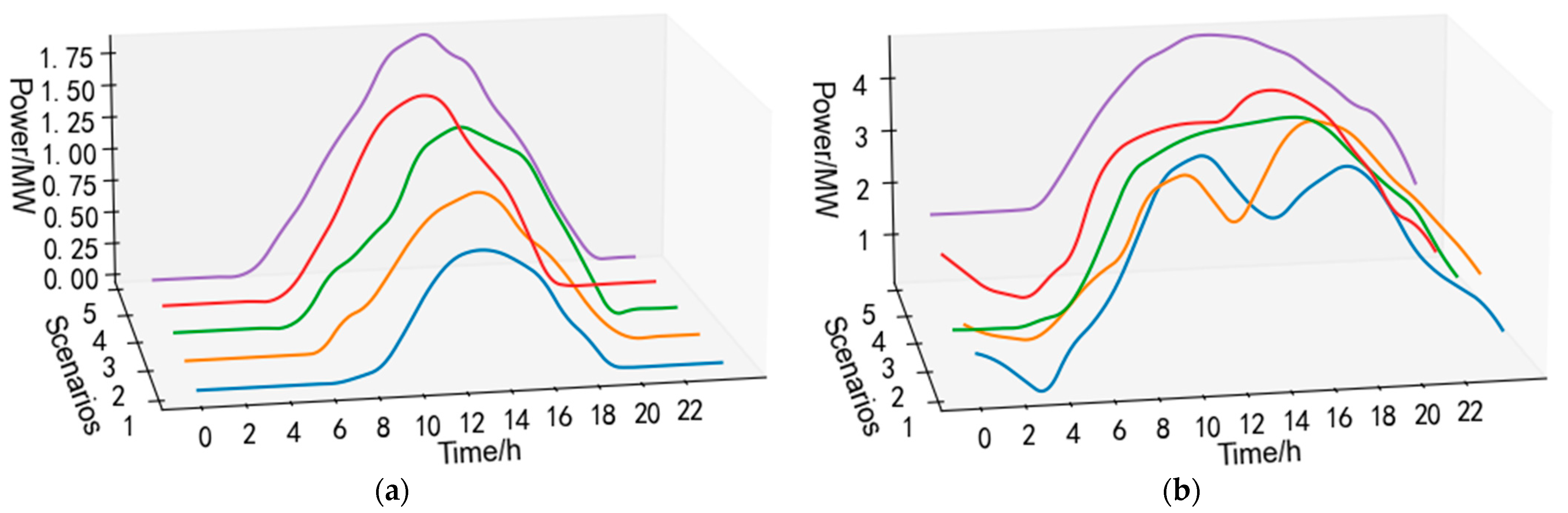
Figure 3. According to the annual photovoltaic output and load power in a certain place in Jiangxi, the joint distribution scenario of five photovoltaic power-generation scenarios and five load scenarios was obtained by scene reduction, and the distribution of each scene is shown in
Table 1 and
Figure 4. In
Figure 4, the 5 lines represent PV and load power changes throughout the day under 5 different scenarios. The initial PV units with 450 kVA, 500 kVA, 450 kVA, and 400 kVA capacities are connected to nodes 14, 22, 24, and 31, respectively. Considering that the installation of SOP is limited by geographic location, the installation location for SOP is selected at the connection switch. Additionally, one photovoltaic unit is planned to be installed at node 11. The optimization of SOP, ESS, and PV is conducted based on all typical scenarios, and, finally, the optimized results are validated under a specific scenario of photovoltaic (scenario 3) and load (scenario 1).
In this example, the four access comparison schemes are set as follows:
Scheme 1: Do not install any SOP and ESS;
Scheme 2: Install a set of SOP and ESS at random locations;
Scheme 3: The system optimizes access to one set of SOP and one set of ESS.
Scheme 4: The system optimizes access to two sets of SOP and two sets of ESS.
The four schemes are progressively advanced and compared with each other. Scheme 1 directly uses the SSGA algorithm to solve the access photovoltaic capacity. Scheme 2 randomly selects the installation positions of SOP and ESS to determine the installation capacity of each device. Scheme 3 and Scheme 4 use the SOCP-SSGA hybrid algorithm to optimize the installation of SOP, ESS, and PV, resulting in optimal economic cost and access to distributed photovoltaic capacity for each scenario in the distribution network cycle. Finally, draw the voltage diagram of each node and the running-state diagram of each device in a typical scenario (photovoltaic scenario 3 and load scenario 1).
Table 2 shows the parameters in the distribution network system planning.
5.2. Comparative Analysis of Optimization Schemes
No SOP and ESS were installed in the system and a photovoltaic unit was connected at node 11. The SSGA algorithm was used to optimize the photovoltaic access capacity and calculate the economic components. The optimized PV capacity and economic costs are shown in
Table 3 and
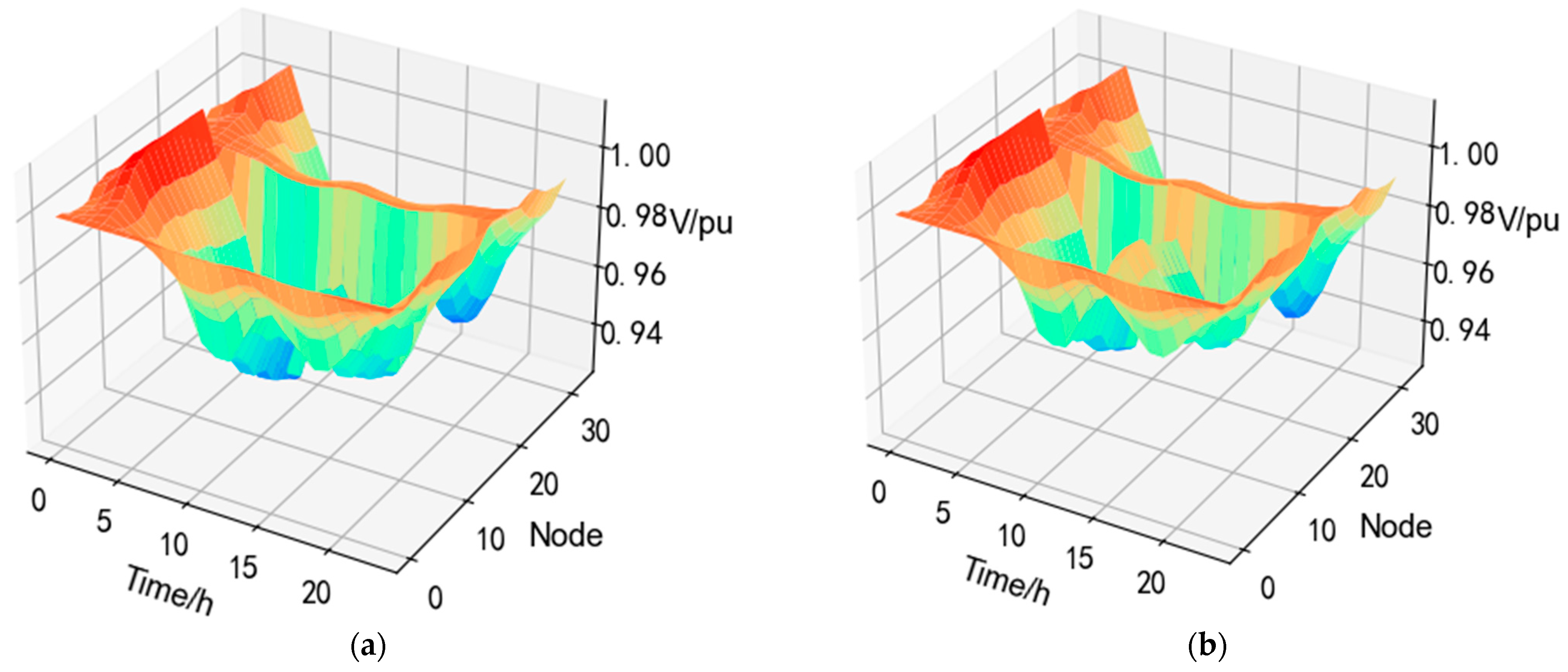
Table 4, respectively. The voltage changes at each node throughout the day before and after the optimization of PV are shown in
Figure 5a,b.
As can be seen from
Figure 5, PV access raises the voltage near the access node, but the overall voltage value is low.
- 2.
Scheme 2
A set of SOP and ESS are installed at random locations. The random installation location of SOP is between nodes 12 and 22; the random access to ESS is node 15; and a group of photovoltaic units are connected at node 11, and the access capacity of each component is solved by the optimization algorithm optimization. The configuration and economic cost of each capacity after optimization are shown in
Table 5 and
Table 6. The voltage changes at each node throughout the day before and after the optimization of PV are shown in
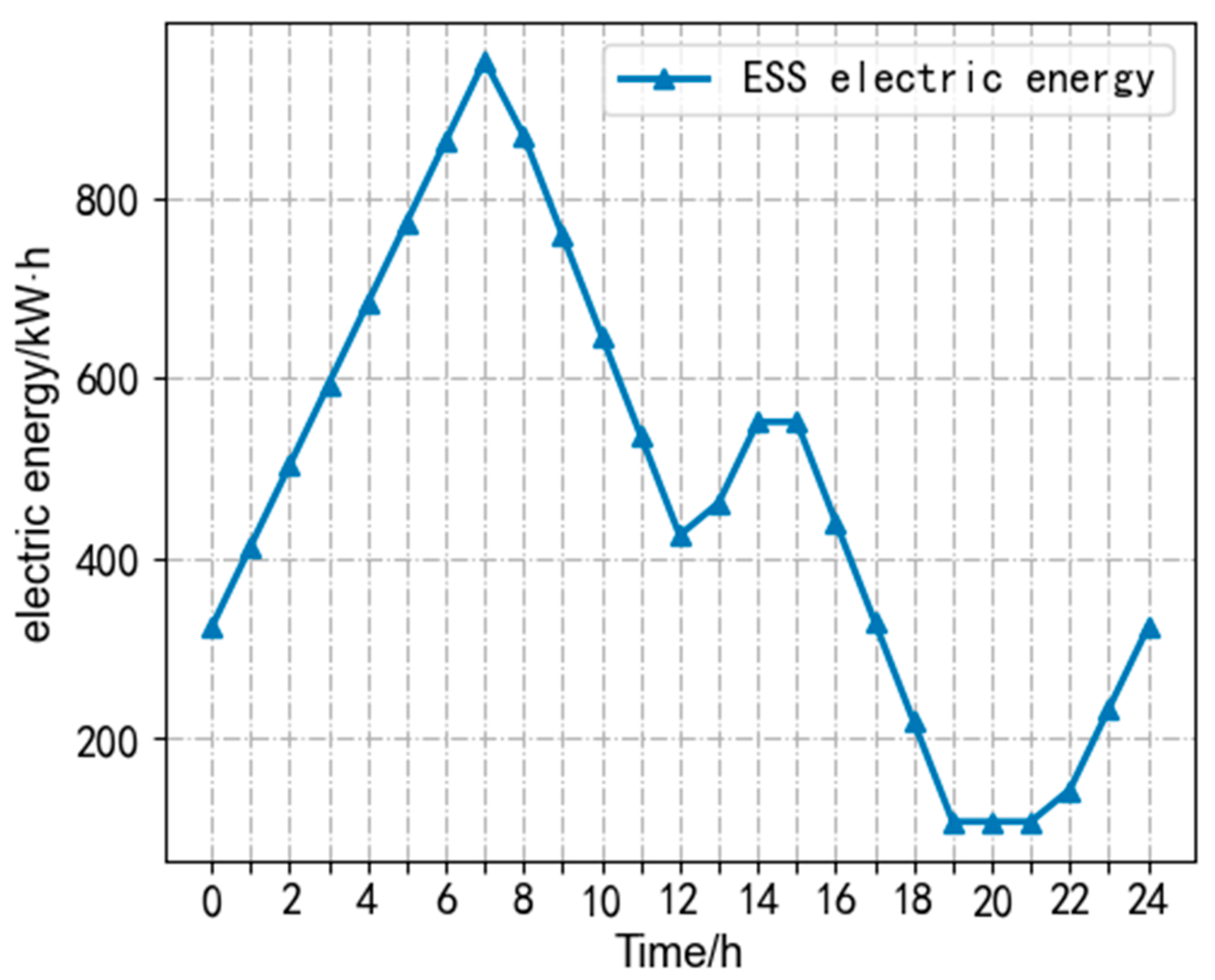
Figure 6a,b. The active power output and reactive power compensation of the SOP during daily operation after optimization are shown in
Figure 7a,b, and the daily operating energy of the ESS is shown in
Figure 8.
From
Figure 6, it can be seen that the installation of SOP and ESS changes the voltage distribution at each node, while the installation of photovoltaic units raises the voltage at each node. From
Figure 4 and
Figure 7, it can be seen that during the time periods of 6:00–11:00 and 14:00–19:00, when the system load is high, SOP provides reactive power compensation to balance the power distribution in the system. As can be seen from
Figure 8, ESS will charge before the peak load, and supply power to the grid after the peak to balance the load burden. The charging power is low at 14:00 because the PV output power is high at this time and the load is lower than in the morning session, therefore, the demand for ESS power is correspondingly reduced.
- 3.
Scheme 3
The system installed one set of SOP and ESS each and a set of photovoltaic units was installed at node 11. After optimization using the SOCP-SSGA algorithm, the optimal positions for SOP and ESS were determined to be between nodes 8 and 21 and at node 13, respectively. After optimization, the configuration and economic cost of each capacity are shown in
Table 7 and
Table 8. The voltage changes at each node before and after PV optimization are shown in
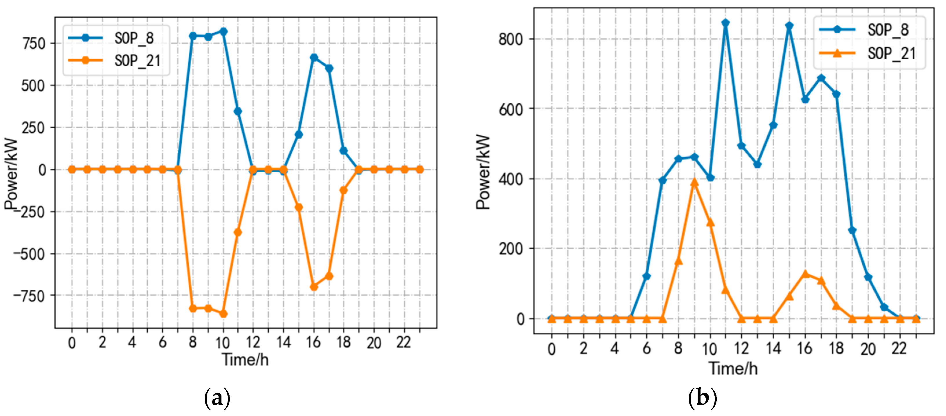
Figure 9a,b, respectively. The daily active power output and reactive power compensation of SOP after optimization are shown in
Figure 10a,b, respectively, and the daily operation of ESS is shown in
Figure 11.
After SOCP-SSGA is used to optimize the position and capacity in Scheme 3, the operation trend of various system indicators is roughly the same as that in Scheme 2. Moreover, due to reasonable access of SOP and ESS, SOP can provide more accurate reactive power compensation for the system, and after PV is connected to the system, the system voltage fluctuation is small, and various economic indicators of the system are better after optimization.
- 4.
Scheme 4
Two sets of SOP and ESS were installed in the system and one set of PV units was installed at node 11. Based on the optimized location in Scheme 3, the SOCP-SSGA algorithm was used for further optimization. The results showed that the new SOP access points were between nodes 18 and 33, while the ESS access point was at node 25. The optimized capacity configuration and economic cost are shown in
Table 9 and
Table 10, respectively. The voltage changes over a day at each node before and after PV optimization are shown in
Figure 12a,b, respectively. The active power output and reactive power compensation of the optimized SOP are shown in
Figure 13a,b and the ESS operating power is shown in
Figure 14.
From
Figure 12, it can be seen that as the number of SOP increases, Scheme 4 significantly improves the voltage quality of the distribution network, with voltage values at each node closer to the per-unit value. It can be observed from
Figure 12 that the addition of SOP leads to a wider range of reactive power regulation time for Node 33. This is because the new PV is connected to a different feeder than Node 33, and Node 33 has a higher demand for load in the system. Therefore, SOP provides reactive power compensation to better utilize solar energy to regulate voltage and improve system stability.
From the ESS operating energy diagram in each scheme, it can be seen that the distribution network will store energy in the ESS during low load power, and as the load power increases, the ESS releases energy to balance the power load and improve power quality. With the increase of the number of ESS, the new ESS added will share the power system demand with the initial ESS so the installation capacity of the initial ESS can be appropriately reduced, and with the increase of the number of SOP, the regulating ability of the system by SOP becomes more prominent so the ESS access capacity can be further reduced. Similarly, with the increase in the number of SOP, adding a new SOP will reduce the initial SOP capacity, and multiple SOPs can cooperate to regulate the distribution-network system, and the voltage level is significantly improved.
Four schemes were compared and analyzed. In Scheme 1, the SOP and ESS are not connected to the system. When compared with this scheme, it was found that in Scheme 2, after the SOP and ESS were randomly connected, the PV capacity of the distribution network was increased from 3.7865 MW to 4.3254 MW, while the fault-loss cost decreased from RMB 78,965 to RMB 56,928. Therefore, it can be concluded that connecting the SOP and ESS significantly increases the PV access capacity and reduces the fault-loss cost.
In Scheme 3, the system optimizes access to a set of SOP and ESS and, compared with the random access of the Scheme 2 system, it can be found that the installation location and capacity of SOP and ESS after the optimization of Scheme 3 are better, mainly reflected in the fact that the system-failure loss cost after optimization is reduced from RMB 56,928 to RMB 30,117, the total economic cost is reduced from RMB 447,988 to RMB 386,259, and the PV capacity is increased from 4.3254 MW to 4.8532 MW.
With the increase in the number of Sops and ESS installed in Scheme 4, compared with the single access Sops and ESS in Scheme 3, the investment, operation, and maintenance cost of multiple Sops and ESS is lower than the investment and operation and maintenance cost of single access Sops and ESS. The fundamental reason is that multiple Sops and ESS can coordinate different locations of the distribution network, thus easing the adjustment pressure required for a single access. In addition, with the increase in the number of ESS and SOP access, the fault-loss cost and power-loss cost of the distribution network decreased significantly, the fault loss cost decreased from RMB 30,117 to RMB 23,506, and the power loss cost decreased from RMB 42,150 in the single optimized access to RMB 18,000. The PV access capacity increased from 4.3254 MW to 6.4283 MW and the access capacity was significantly improved.


