Article

Observer-Based Approximate Affine Nonlinear Model Predictive Controller for Hydraulic Robotic Excavators with Constraints

1
School of Mechanical and Electrical Engineering, Central South University, Changsha 410083, China
2
State Key Laboratory of Precision Manufacturing for Extreme Service Performance, Changsha 410083, China
3
Sunward Intelligent Equipment Co., Ltd., Changsha 410100, China
*
Author to whom correspondence should be addressed.
Processes 2023, 11(7), 1918; https://doi.org/10.3390/pr11071918
Submission received: 17 May 2023 / Revised: 19 June 2023 / Accepted: 23 June 2023 / Published: 26 June 2023

Abstract

:
Given the highly nonlinear and strongly constrained nature of the electro-hydraulic system, we proposed an observer-based approximate nonlinear model predictive controller (ANMPC) for the trajectory tracking control of robotic excavators. A nonlinear non-affine state space equation with identified parameters is employed to describe the dynamics of the electro-hydraulic system. Then, to mitigate the plant-model mismatch caused by the first-order linearization, an approximate affine nonlinear state space model is utilized to represent the explicit relationship between the output and input and an ANMPC is designed based on the approximate nonlinear model. Meanwhile, the Extended Kalman Filter was introduced for state observation to deal with the unmeasurable velocity information and heavy measurement noises. Comparative experiments are conducted on a 1.7-ton hydraulic robotic excavator, where ANMPC and linear model predictive control are used to track a typical excavation trajectory. The experimental results provide evidence of convincing trajectory tracking performance.

1. Introduction

Robotic excavators are a type of multi-joint device driven by hydraulic systems, which are widely used in earth-moving fields such as energy development, road construction, and infrastructure construction. However, the operator must have skilled techniques to control the multiple joints of the excavator to improve operational efficiency [1]. In addition, in some harsh construction environments, the operator’s safety may be threatened. As a consequence, it is very difficult for manual operation to meet the requirements of excavation operations. In this regard, the automation of excavators has attracted a great deal of interest, which can help reduce human-associated costs and improve construction efficiency and safety [2,3].
Excavator automation can be viewed as the control of a kind of robot with a bucket as an end effector, and trajectory tracking control is the key to automated operations [4]. However, since robotic excavators typically use hydraulic systems as their power source, achieving high-performance trajectory tracking remains challenging due to the nonlinear and multi-constrained features [5]. Many control methods, such as the improved PID control [6,7,8], self-tuning pressure-feedback control [9], adaptive robust control [10], intelligent control [11,12], and so on, have been proposed to deal with the nonlinearity, time-variance, and parameter uncertainty of hydraulic robotic excavators. However, they find it difficult to meet the multi-constraint features of electro-hydraulic systems [13]. In practical applications, hydraulic actuators face various constraints, such as control input constraints, speed constraints, and position constraints. A control strategy that neglects physical constraints may degrade the control performance and even lead to system instability [14,15].
Due to the presence of constraints in hydraulic systems, the MPC method has become an increasingly popular control strategy. As an optimal control technique, MPC can actively handle system constraints during the control process, showing great potential in solving complex system control problems with strong constraints [16]. In [17], a hybrid control method consisting of linear model predictive control (MPC) and proportion-integration control (PIC) was proposed for force control of electro-hydraulic servo systems, where the MPC in the outer loop provided references to the PIC in the inner loop. For the trajectory tracking control of a robotic excavator, a linear MPC was designed in [18,19] with simulation and experimental verification. In [20], a gain-scheduled MPC was proposed for the dynamic performance enhancement of an excavator, but only the boom joint was considered. All aforementioned MPC-based controllers are based on linear models, because nonlinear MPC has the limitation of heavy online computation burden, requiring extensive computational resources and longer solving times, making it difficult to apply in practical robotic excavators [21]. Nevertheless, due to the presence of dead zones, saturation, nonlinear friction, and the compressibility of hydraulic oil, hydraulic systems have complex nonlinear dynamics [13]. Consequently, linear models based on the first-order linearization of the nonlinear system using Jacobian calculations will introduce large errors, resulting in control performance degradation [22].
On the other hand, the MPC control method adopts the concept of full-state feedback control, which means that all state information (i.e., position signals, velocity signals, and pressure signals) must be known during the control process [23]. However, for most hydraulic excavators, not all system states can be directly measured due to physical limitations or the high cost of implementing enough sensors. In addition, the heavy noise in the measurement may cause inaccurate state information. Based on the above considerations, state observers have received considerable attention, such as the Extended State Observer [24], Sliding Mode Observer [25], and State-Dependent-Riccati-Equation filter [26]. Among these observers, the Extended Kalman Filter (EKF) has been widely used as a state estimator in nonlinear systems, providing a simple and effective solution to the state estimation problem of complex nonlinear systems [27,28]. Within this context, only pressure and displacement sensors are installed for the robotic excavator. Therefore, we design an EKF for the electro-hydraulic system to estimate the unknown velocity information while reducing the measurement error of displacement and pressure signals.
Motivated by the above challenges, an observer-based approximate nonlinear model predictive controller is proposed for a hydraulic robotic excavator in this study. The main contributions of this paper are as follows.
(1)
Parameter identification was performed to identify the key parameters in the nonlinear non-affine model of the hydraulic excavator using measured data. Then, the nonlinear non-affine model is approximated to an affine nonlinear state-space model, which can reduce unmodeled errors and more accurately reflect the system’s dynamic features compared to the conventional first-order linearization models.
(2)
An approximated nonlinear model predictive control (ANMPC) is designed based on the approximate affine nonlinear state-space model, which can still be solved by quadratic programming (QP), with the same computation burden as a linear MPC, avoiding solving the nonlinear MPC problem. As only pressure and displacement sensors are installed for the robotic excavator, we design an EKF observer for the electro-hydraulic system to estimate the unknown velocity information while reducing the measurement error of displacement and pressure signals.
(3)
Experiments were conducted on a 1.7-ton hydraulic excavator, where three joints of the hydraulic excavator were simultaneously controlled to execute a typical excavation trajectory. The results demonstrate that the proposed observer-based ANMPC outperforms the conventional LMPC in trajectory tracking control during excavation.
The rest of this article is organized as follows. The working principle of electro-hydraulic excavator is introduced in Section 2, a non-affine nonlinear mathematical model of the electro-hydraulic excavator is established, and a parameter identification is performed to obtain the unknown parameters. In Section 3, an approximate nonlinear model predictive controller with an EKF for the electro-hydraulic excavator is designed. Section 4 presents the trajectory tracking control results based on a 1.7-ton robotic excavator. The conclusions of this study are given in Section 5.

2. System Description and Modeling

2.1. Electro-Hydraulic System Description

A 1.7-ton electro-hydraulic robotic excavator is used in this study, and the flow coupling between different hydraulic cylinders is ignored. As the boom, stick, and bucket are theoretically the same, we establish an electro-hydraulic control system model using the bucket as an example. As shown in Figure 1, the electro-hydraulic control system primarily consists of a controller, a pilot valve, a main valve, and hydraulic cylinders. The working principle is as follows. According to the reference trajectory and the actual position, the controller generates a control signal, which is amplified and used to control the pilot valve. According to the given control signal, the pilot valve will push the spool of the main valve to move to the left or right, connecting the corresponding pipeline with the cavity of the hydraulic cylinder. Then, the piston rod will extend or retract under the push of hydraulic oil, thus realizing the movement of the cylinder. The actual position of the cylinder during movement will be fed back to the controller through a displacement sensor, to form a closed control loop.

2.2. Kinematics

The kinematic model of the excavator robot plays a crucial role in determining the relationship between joint angles and end-effector positions, which is essential for trajectory planning and control. The D-H coordinate system of the robotic excavator is established as shown in Figure 2. The D-H coordinate parameters are shown in Table 1.
We can derive the forward kinematics equations to calculate the end-effector pose  [ p x , p y , p z , ψ ]  from the joint angles  [ θ 1 , θ 2 , θ 3 , θ 4 ] , which is presented as Equation (1):
p x = cos ( θ 1 ) [ a 4 cos ( θ 2 + θ 3 + θ 4 ) + a 3 cos ( θ 2 + θ 3 ) + a 2 cos ( θ 2 ) + a 1 ] p y = sin ( θ 1 ) [ a 4 cos ( θ 2 + θ 3 + θ 4 ) + a 3 cos ( θ 2 + θ 3 ) + a 2 cos ( θ 2 ) + a 1 ] p z = a 4 sin ( θ 2 + θ 3 + θ 4 ) + a 3 sin ( θ 2 + θ 3 ) + a 2 sin ( θ 2 ) + d 1 ψ = θ 2 + θ 3 + θ 4
The inverse kinematics equations can also be derived to calculate the joint angles required to achieve a desired end-effector position and orientation. The angles of each joint  θ 1 θ 4  can be calculated by Equation (2):
θ 1 = atan ( p y p x ) θ 2 = α + β + γ θ 3 = π acos ( a 2 2 + a 3 2 C Q 2 2 a 2 a 3 ) θ 4 = ψ θ 2 θ 3
where  α  is the angle between CF and the horizontal line,  β  is the angle between CQ and the horizontal line, and  γ  is the angle between CV and the horizontal line.

2.3. Mathematical Model of EHS

Usually, the response speed of the pilot valve is much faster than that of the main valve, so the dynamic characteristics of the pilot valve can be ignored without significantly reducing control performance [7,8]. Therefore, this process can be regarded as a pure proportional stage:
x v = k v I
where  x v  is the spool displacement of the main valve,  I  is the control current, and  k v  is a coefficient.
The following equation expresses the orifice flow equation in the main valve:
Q L = C d ω x v P s s g n ( x v ) P L ρ
where  Q L  is the load flow,  P L  is the load pressure,  C d  is the discharge coefficient,  ω  is the spool valve area gradient,  ρ  is the fluid mass density,  P s  is the supply pressure, and  s g n ( )  is the symbolic function.
Ignoring the external leakage of the hydraulic cylinder, the continuity equation of the hydraulic cylinder flow can be expressed as:
A y ˙ + C t P L + V t 4 β e P ˙ L = Q L
where  A  is the cross-sectional area of the cylinder,  y  is the displacement of the piston rod,  V t  is the total actuator volume,  C t  is the coefficient of leakage, and  β e  is the effective bulk modulus.
The force balance equation of the hydraulic cylinder is:
P L A = m y ¨ + b y ˙ + k y + F f
where  m  is the equivalent mass,  b  is the viscous damping coefficient,  k  is the equivalent spring stiffness, and  F f  is the friction force. In our study, the coulomb viscous model is selected to describe the frictional force acting on hydraulic cylinders:
F f = F c + F v d ˙
where  F c  is the stiction force and  F v  is the dynamic friction coefficient.
Combining the above equations of each sub-system, selecting the state vector  [ x 1 ; x 2 ; x 3 ] = [ y ; y ˙ ; P L ]  and the control input  u = I , the model of an electro-hydraulic system can be represented by the following three non-affine nonlinear state space equations:
x ˙ 1 = x 2 x ˙ 2 = k m x 1 b m x 2 + A m x 3 F c s g n ( x 2 ) + F v x 2 m x ˙ 3 = 4 A β e V t x 2 4 C t β e V t x 3 + 4 C d β e ω k v V t ρ P s s g n ( u ) x 3 u
Equation (8) can be rewritten as:
x ˙ 1 = x 2 x ˙ 2 = a 1 x 1 a 2 x 2 + a 3 x 3 a 4 s g n ( x 2 ) x ˙ 3 = a 5 x 2 a 6 x 3 + a 7 P s s g n ( u ) x 3 u
where,  a 1 = k m a 2 = b + F v m a 3 = A m a 4 = F c m a 5 = 4 A β e V t a 6 = 4 C t β e V t , and  a 7 = 4 C d β e ω k v V t ρ .
We selected the sampling time as  T s  and the system output as  y ( k ) = x 1 ( k ) . Then, the discrete state space equation model can be obtained through forward difference discretization:
x 1 ( k + 1 ) = T s x 2 + x 1 ( k ) x 2 ( k + 1 ) = a 1 x 1 ( k ) a 2 x 2 ( k ) + a 3 x 3 ( k ) a 4 s g n ( x 2 ( k ) ) T s + x 2 ( k ) x 3 ( k + 1 ) = a 5 x 2 ( k ) a 6 x 3 ( k ) + a 7 P s s g n ( u ( k ) ) x 3 ( k ) u ( k ) T s + x 3 ( k )

2.4. Model Validation

To estimate the model parameters, a pseudo-random binary signal (PRBS) with a range of [−200 mA, 200 mA] is selected as the excitation for parameter identification, as shown in Figure 3a. We construct nonlinear grey-box modeling of EHS using the System Identification Tool in MATLAB. The settings of grey-box parameter identification [17] are as follows: The solver was the Runge-Kutta 45 solver with an adaptive step size, the search method was the Trust-Region Reflective Newton method of nonlinear least squares, the cost function was set as the sum of squared error between the measured output and simulated output, and the absolute error and relative error tolerances were 1 × 10⁻⁶ and 1 × 10⁻⁵, respectively. The parameter identification results are given in Table 2. Under this set of parameters, model outputs fit 98.48% of actual system outputs and the final prediction of the error is 1.57 × 10⁻⁷, and the comparison between the model response and the actual data is shown in Figure 3b. Thus, we ensure that the results of parameter identification are reasonable.
To verify the estimated mathematical model, we tested the real system with mixed sine signals of different frequencies, as given in Equation (11). Subsequently, we compared the experimental results with the model output. Figure 4b shows that the response of the model agreed well with the experimental data, indicating that the identified model can accurately predict the behavior of the real system.
u ( t ) = 80 + 20 [ sin ( 4 π t ) + sin ( 2.6 π t ) + sin ( 2 π t ) + sin ( 1.6 π t ) + sin ( 0.8 π t ) ] , t 15 120 30 [ sin ( 2 π t ) + sin ( 1.3 π t ) + sin ( π t ) + sin ( 0.8 π t ) + sin ( 0.4 π t ) ] , t > 15
As an example, the identification results of the bucket are listed in Table 2. Similarly, we can obtain the parameters for the boom and arm, as shown in Table 3.

3. Approximate Nonlinear Model Predictive Controller Design

The design of an MPC controller requires a model to predict the future state and obtain the optimal control input by solving an optimization problem in real-time [21]. Therefore, accurate modeling of a system is crucial for an MPC controller. The electro-hydraulic system is highly nonlinear, but the design of the NMPC controller will cause difficulties in solving optimization problems and bring a large computational burden. Therefore, linearization methods are often used to obtain the linear expression of the model, and an LMPC will be designed based on it.
Usually, the linearization method involves computing the Taylor expansion of the model at the equilibrium point and ignoring the higher-order terms. However, the first-order linearization introduces unmodeled errors, thus the linearized model cannot accurately reflect the dynamic characteristics of the system. When the equilibrium is improperly selected, it can lead to a decrease in controller performance or even cause the control system to diverge. Therefore, to reduce the plant-model mismatch caused by linearization, this study uses an approximate method to represent the explicit relationship between the output and input.

3.1. Approximation Affine Nonlinear State Space Model

Due to the nonlinear relationship between the input and output, it is difficult to derive the relationship between the output and the input and design a predictive controller. Therefore, an approximate model is first derived for System (9) to ensure a simplified input–output relationship. For the non-affine nonlinear model  i , where  i = b o o m , a r m , b u c k e t  in this study, the Taylor expansion of  x i ( k + 1 )  with respect to  u i ( k )  around  u i ( k 1 )  is shown as:
x i ( k + 1 ) = f i [ x i ( k ) , u i ( k 1 ) ] + f i [ x i ( k ) , u i ( k 1 ) ] u i ( k ) ( u i ( k ) u i ( k 1 ) ) + ε i ( k )        = f i [ x i ( k ) , u i ( k 1 ) ] + g i [ x i ( k ) , u i ( k 1 ) ] Δ u i ( k ) + ε i ( k )
where  ε i ( k ) = 2 f i [ x i ( k ) , μ i ( k ) ] u i 2 ( k ) Δ u i 2 ( k )  and  μ i ( k ) = η i u i ( k ) + ( 1 η i ) u i ( k 1 )  with  η i  being a positive constant.
Since only the derivative expansion of the control input is performed, the nonlinear characteristics of the state variables are retained. Subsequently, the approximate model may not miss too many characteristics of the system [27,29].

3.2. ANMPC Design

Ignoring  ε i ( k )  in Equation (12), an approximate affine nonlinear system can be represented by state space Equation (13):
x i ( k + 1 ) = f i [ x i ( k ) , u i ( k 1 ) ] + g i [ x i ( k ) , u i ( k 1 ) ] Δ u i ( k )   y i ( k ) = C x i ( k )
with constraints:
u i , m i n u i ( k ) u i , m a x Δ u i , m i n Δ u i ( k ) Δ u i , m a x y i , m i n y i ( k ) y i , m a x
where  x i ( k ) n x  is the state vector,  u i ( k ) n u  is the input vector,  y i ( k ) n y  is the output vector,  Δ u i ( k )  is the input increment,  f i ( )  and  g i ( )  are nonlinear functions, and  u i , m i n u i , m a x Δ u i , m i n Δ u i , m a x , and  y i , m i n y i , m a x  are vectors of lower and upper bounds and  C = [ 1 , 0 , 1 ] .
Note that there are two main reasons why we ignore the second-order term  ε i ( k ) . Firstly, the output of a physical system in practice cannot change too fast within a small time interval due to the “inertia” of the system [26,28], which means that  Δ u i ( k )  is limited. Secondly, when the reference trajectories to be tracked are constant, the approximation error  ε i ( k )  will approach zero because  Δ u i ( k ) 0  in the steady state. In addition, the mechanism of a receding horizon and repeating optimization gives MPC inherent robustness.
The MPC controller is an iterative optimization technique, and at each sampling time k, the optimal control input is obtained by solving the optimization problem online based on the current system states and references, and the first element of the control sequence will be applied to the system. The optimal control input is obtained by continuously solving the following optimization problem:
min Δ u i ( k ) J i ( k ) = j = 1 N p r i ( k + j | k ) y i ( k + j | k ) Q 2 + j = 0 N m 1 Δ u i ( k ) W 2
where  r i ( k + j | k )  is the reference,  N p  and  N m  are the prediction horizon and the control horizon, respectively,  N m N p , Q, and W are weighting matrices for two optimization terms, and  2  denotes the Euclidean norms of vectors.
The first term in Equation (14) represents the error between the predicted output and the reference, while the second term considers the change in the control input. According to the approximate affine non-linear Model (13), we have:
x i ( k + 1 k ) = f i [ x i ( k | k 1 ) , u i ( k 1 ) ] + g i [ x ( k | k 1 ) , u i ( k 1 ) ] Δ u i ( k ) x i ( k + 2 k ) = f i [ x i ( k + 1 | k 1 ) , u i ( k 1 ) ] + g i [ x ( k + 1 | k 1 ) , u i ( k 1 ) ] ( Δ u i ( k ) + Δ u i ( k + 1 ) )    x i ( k + N p k ) = f i [ x i ( k + N p 1 | k 1 ) , u i ( k 1 ) ] + g i [ x ( k + N p 1 | k 1 ) , u i ( k 1 ) ] ( Δ u i ( k ) +          + Δ u i ( k + N m 1 ) )
Define the following vectors:
Y i = [ y i ( k + 1 k )   , y i ( k + 2 k )   ,   y i ( k + N p k ) ] N p n y
R i = [ r i ( k + 1 k )   , r i ( k + 2 k )   ,   r i ( k + N p k ) ] N p n y
Δ U i = [ Δ u i ( k )   , Δ u i ( k + 1 ) ,     Δ u i ( k + N m 1 ) ] N m n u
X i = [ x i ( k + 1 k ) ,   x i ( k + 2 k )   ,   x i ( k + N p k ) ] N p n x
Transforming recursive Equation (14) into matrix form, we have:
Y i = C ¯ X i = C ¯ ( F i + G i Δ U i )
where:
C ¯ = C 0 0 C N p n y × N p n x
F i = f i [ x ( k ) , u ( k 1 ) ] f i [ x ( k + 1 k ) , u ( k 1 ) ] f i [ x ( k + p 1 k ) , u ( k 1 ) ] N p n x
G i = g i [ x ( k | k 1 ) , u i ( k 1 ) ] 0 0 g i [ x ( k | k 2 ) , u i ( k 1 ) ] g i [ x ( k + 1 | k 1 ) , u i ( k 1 ) ] 0 g i [ x ( k + N p 1 k 1 ) , u i ( k 1 ) ] g i [ x ( k + N p 1 k 1 ) , u i ( k 1 ) ] g i [ x ( k + N p 1 k 1 ) , u i ( k 1 ) ] N p n x × N m n u
Hence, the original optimization Problem (14) becomes:
min Δ U i J i ( k ) = R i Y i Q 2 + Δ U i W 2        = R i C ¯ F i C ¯ G i Δ U i Q 2 + Δ U i W 2
s . t . u i , m i n u i ( k 1 ) + Δ U i u i , m a x Δ u i , m i n Δ U i Δ u i , m a x y i , m i n C ¯ ( F i + G i Δ U i ) y i , m a x
The above optimization problem is a standard quadratic programming problem, if the weight matrices W and Q are positive definite, then the objective Function (21) is strictly convex, and the feasible region defined by the constraints is a closed convex set. Therefore, the solution to Equation (21) is unique and satisfies the Karush–Kauhn–Tucker (KKT) conditions [30,31].

3.3. EKF-Based ANMPC Design

For the MPC method, the full-state feedback control concept is adopted, which means that all state information (i.e., position signal, velocity signal, and pressure signal) should be available in electro-hydraulic system control. However, in practical systems, due to limitations in installation conditions and cost, not all state information can be obtained through sensors directly. In this study, the displacement and pressure signals of hydraulic cylinders can be obtained through sensors. In terms of the velocity signal, the Extended Kalman Filter (EKF) is introduced as a state observer, which is one of the most popular state estimation techniques primarily developed for nonlinear systems [32]. In addition, the EKF is capable of correcting the position and pressure signals to reduce noise, which further improves the accuracy of the state estimation.
For the nonlinear System (10), the EKF of model i is implemented as follows:
x ^ i ( k + 1 ) = f i ( x ^ i ( k ) , u i ( k ) ) + K i ( k ) ( y i ( k + 1 ) H f i ( x ^ i ( k ) , u i ( k ) ) ) K i ( k + 1 ) = P i ( k + 1 ) H T ( H P i ( k ) H T + R F , i ( k ) ) 1 P i ( k + 1 ) = F i ( k ) ( P i ( k ) P i ( k ) H T ( H P i ( k ) H T + R i ( k ) ) 1 H P i ( k ) ) F i ( k ) T + Q F , i ( k )
where  F i ( k ) = f i ( x i ( k ) , u i ( k ) ) x i ( k ) x i ( k ) = x ^ i ( k ) H  represents the measurement matrix,  Q F , i ( k )  and  R F , i ( k )  are the noise matrix of model and observation, and the choice of  Q F , i ( k )  and  R F , i ( k )  can be found in [27,32]. The stability problem of the Kalman filter can be found in [28].
We defined the observer error of EKO as  ξ i ( k ) = x i ( k ) x ^ i ( k ) , then:
ξ i ( k + 1 ) = x i ( k + 1 ) x ^ i ( k + 1 )        = ( I K i ( k + 1 ) H ) f i ( η i ( k ) , u i ( k ) ) x i ( k )
where  η i ( k ) [ x i ( k ) , x ^ i ( k ) ] . According to [32],  ξ i ( k ) T p i ( k + 1 ) 1 ξ i ( k )  is a decreasing sequence and thus  ξ i ( k ) 0  as  k .
After introducing the Kalman state observer, Equation (14) can be represented by:
  x ^ i ( k + 1 k ) = f i [ x ^ i ( k | k 1 ) , u i ( k 1 ) ] + g i [ x ^ ( k | k 1 ) , u i ( k 1 ) ] Δ u i ( k ) x ^ i ( k + 2 k ) = f i [ x ^ i ( k + 1 | k 1 ) , u i ( k 1 ) ] + g i [ x ^ ( k + 1 | k 1 ) , u i ( k 1 ) ] ( Δ u i ( k ) + Δ u i ( k + 1 ) )    x ^ i ( k + N p k ) = f i [ x ^ i ( k + N p 1 | k 1 ) , u i ( k 1 ) ] + g i [ x ^ ( k + N p 1 | k 1 ) , u i ( k 1 ) ] ( Δ u i ( k ) +          + Δ u i ( k + N m 1 ) )
Then, Equations (19) and (20) become:
X ^ i = [ x ^ i ( k + 1 k ) ,   x ^ i ( k + 2 k )   ,   x ^ i ( k + N p k ) ] N p n x
Y i = C ¯ X ^ i = C ¯ ( F ^ i + G ^ i Δ U i )
where:
F ^ i = f i [ x ^ ( k ) , u ( k 1 ) ] f i [ x ^ ( k + 1 k ) , u ( k 1 ) ] f i [ x ^ ( k + p 1 k ) , u ( k 1 ) ] N p n x
G ^ i = g i [ x ^ ( k | k 1 ) , u i ( k 1 ) ] 0 0 g i [ x ^ ( k | k 2 ) , u i ( k 1 ) ] g i [ x ^ ( k + 1 | k 1 ) , u i ( k 1 ) ] 0 g i [ x ^ ( k + N p 1 k 1 ) , u i ( k 1 ) ] g i [ x ^ ( k + N p 1 k 1 ) , u i ( k 1 ) ] g i [ x ^ ( k + N p 1 k 1 ) , u i ( k 1 ) ] N p n x × N m n u
Thus, the optimization problem Equation (21) can be rewritten as:
min Δ U i J i ( k ) = R i Y i Q 2 + Δ U i W 2        = R i C ¯ F ^ i C ¯ G ^ i Δ U i Q 2 + Δ U i W 2
s . t . u i , m i n u i ( k 1 ) + Δ U i u i , m a x Δ u i , m i n Δ U i Δ u i , m a x y i , m i n C ¯ ( F i + G i Δ U i ) y i , m a x
In summary, for the electro-hydraulic control system of a single joint i, the overall ANMPC framework is shown in Figure 5.

4. Experiment

4.1. Experiment Platform

Figure 6 shows the experimental platform, which was modified from a 1.7-ton electro-hydraulic excavator. Wire displacement sensors are installed on the hydraulic cylinders to measure the piston rod displacement of the boom, arm, and bucket, and then the position of the bucket tip can be determined by the kinematics of the robot. In addition, six pressure sensors were installed on the joints of the corresponding cylinders to measure the pressure in the rod and non-rod chambers.
The entire control system is divided into the slave part and the master part, which are connected via the CAN bus. The slave part uses a PLC controller primarily for data acquisition and hydraulic system control. The master part uses a computer, and all planning and control algorithms are deployed on the master. Based on the MATLAB GUI environment, the master realizes data reception, display, and the implementation of trajectory planning and trajectory tracking control algorithms.

4.2. Controller Settings

In the experiment, the sampling time of the control system was uniformly set to 0.01 s, which is short enough for the control and the acquisition of data. In order to perform excavation tasks, it is necessary to simultaneously control the boom, stick, and bucket, and the parameters of the three controllers are listed in Table 4.
At the same time, we designed a linear MPC controller for comparison. Unlike ANMPC, the LMPC linearizes system Model (10) at the equilibrium point  ( x i , 0 , u i , 0 ) :
x i ( k + 1 ) = f i ( x i , 0 , u i , 0 ) + f i ( x i , 0 , u i , 0 ) x i ( x i ( k ) x i , 0 ) + f i ( x i , 0 , u i , 0 ) u i ( u i ( k ) u i , 0 ) = A i x i ( k ) + B i u i ( k )
where  A i = f i ( x i , 0 , u i , 0 ) x i B = f ( x 0 , u 0 ) x .
Based on Equation (28), the LMPC can be obtained as:
min Δ U i J i ( k ) = R i Y i Q 2 + Δ U i W 2        = R i S i x i ( k ) V i u i ( k 1 ) M i Δ u i ( k ) Q 2 + Δ U i W 2
s . t . Δ U i , min Δ U i Δ U i , max U i , min u i ( k 1 ) + Δ U i U i , max Y i , min Y i Y i , max
where the definitions of Si, Vi, and Mi are referenced in [30,31]. The parameter settings of the LMPC were the same as those of ANMPC in our experiment.

4.3. Trajectory Planning

In the experiment, the excavator did not rotate, so only motion in the X-Z plane was considered. To verify the effectiveness of the proposed controller, a typical excavation trajectory was used as the reference trajectory. A typical excavation process includes penetration, cutting, and loading [33], and the trajectory of the bucket tip is shown in Figure 7. By solving the inverse kinematics, the trajectory of the bucket tip is converted into the trajectory of each joint, as shown in Figure 8.

4.4. Experiment Results

The LMPC and ANMPC were used to control the hydraulic cylinders to move along the planned trajectory, and the actual trajectories of each joint were obtained through sensors. In the experiment, the tracking performance of each controller was analyzed both in joint space and Cartesian space.
In the joint space, the trajectory tracking control results of the boom, arm, and bucket are given in Figure 9, Figure 10 and Figure 11, respectively. When using the LMPC, the maximum tracking errors of each joint are 4.11 × 10⁻³ m, 3.89 × 10⁻³ m, and 2.65 × 10⁻³ m, respectively, while the maximum trajectory tracking errors of each joint are 1.92 × 10⁻³ m, 1.72 × 10⁻³ m, and 2.06 × 10⁻³ m, respectively, when using the ANMPC.
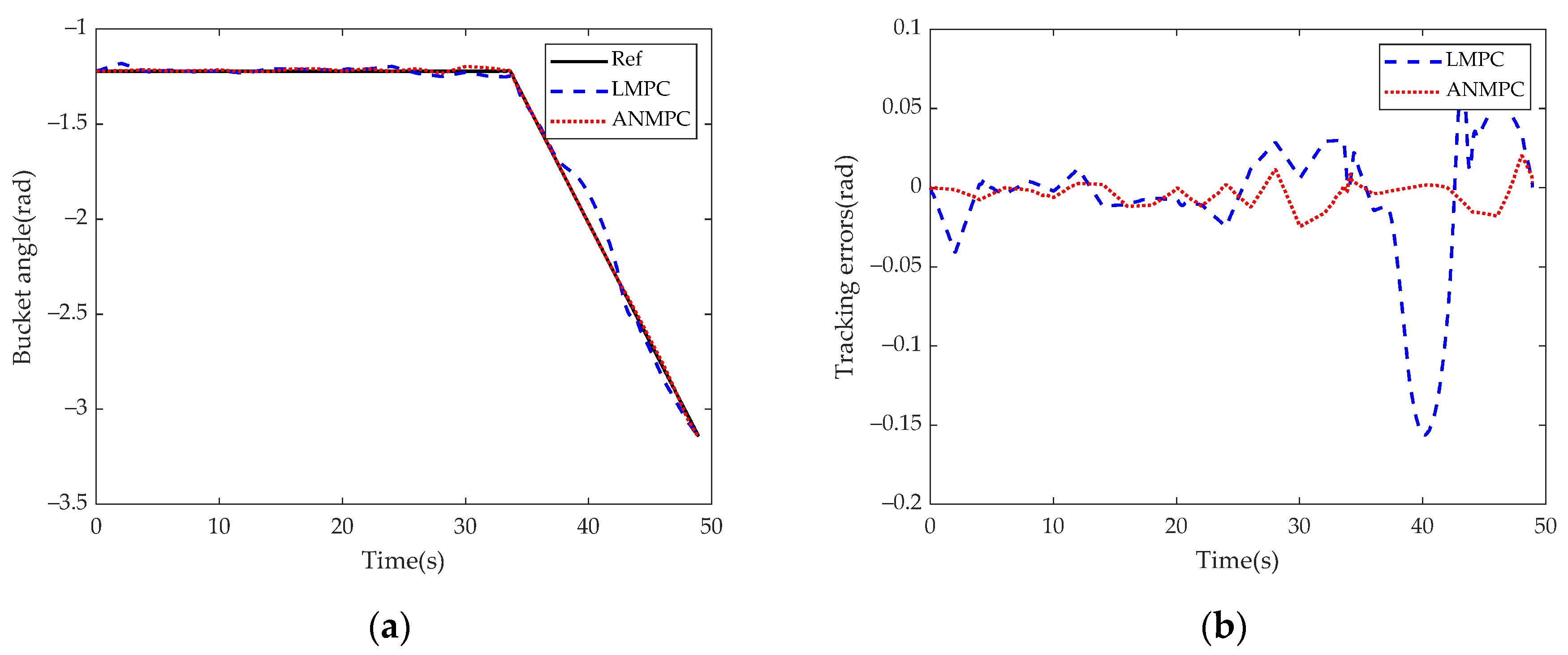
In the Cartesian space, the bucket tip trajectories when using different controllers are shown in Figure 12a, and the position errors are shown in Figure 12b. The maximum errors of the LMPC and ANMPC are 87.5 × 10⁻³ m and 23.1 × 10⁻³ m, respectively. In addition, the tracking performance of the bucket tip in the X-axis, Z-axis, and bucket angle is given in Figure 13, Figure 14 and Figure 15, respectively.
The tracking errors of different controllers when tracking a typical excavation trajectory are shown in Table 5. Due to the less unmodeled error of the approximate affine nonlinear model, the proposed ANMPC has a significant advantage over the LMPC in terms of trajectory tracking control performance of the robotic excavator.

5. Conclusions

In this study, a novel observer-based ANMPC was proposed for the trajectory tracking of a hydraulic robotic excavator. Firstly, considering the highly nonlinear characteristics of the electro-hydraulic system, a non-affine nonlinear system model was established, and the parameters of the model were obtained through a parameter identification method. Then, in order to reduce the plant-model mismatch caused by the conventional first-order linearization, we used an approximation method to obtain the explicit linear relationship between the output and input, and ANMPC is designed based on the approximate affine nonlinear model. Compared with the linearized model, the approximate affine nonlinear state space model can better reflect the dynamic characteristics of the system and predict the future state more accurately. At the same time, ANMPC avoids the difficulties in solving nonlinear MPC problems for non-affine nonlinear systems due to the slow solving speed and insufficient computing resources. Trajectory tracking control experiments were designed on a 1.7-ton excavator platform, where ANMPC and LMPC were used to control the robot to perform a typical excavation trajectory, and the three joints of the robot were controlled simultaneously in the experiment. The experimental results showed that ANMPC had better trajectory tracking control performance than LMPC.
Given the significant external disturbances that robotic excavators face during operation, such as soil resistance, our future work will focus on suppressing disturbances to further improve the performance of the controller and promote its application in engineering. Moreover, combining autonomous navigation and 3D reconstruction to achieve fully autonomous operation is a promising research direction.

Author Contributions

Conceptualization, J.W. and H.D.; methodology, J.W. and H.D.; formal analysis, H.Z. and P.H.; data curation, H.Z.; writing—original draft preparation, J.W.; writing—review and editing, H.D. All authors have read and agreed to the published version of the manuscript.

Funding

Major Science and Technology Project of Changsha City under “the open competition mechanism to select the best candidates”: Kq2102001.

Data Availability Statement

Not applicable.

Conflicts of Interest

The authors declare no conflict of interest.

References

  1. Lee, M.; Choi, H.; Kim, C.; Moon, J.; Kim, D.; Lee, D. Precision Motion Control of Robotized Industrial Hydraulic Excavators via Data-Driven Model Inversion. IEEE Robot. Autom. Lett. 2022, 7, 1912–1919. [Google Scholar] [CrossRef]
  2. Sun, D.; Hwang, S.; Han, J. Lever Control for Position Control of a Typical Excavator in Joint Space Using a Time Delay Control Method. J. Intell. Robot. Syst. 2021, 102, 63. [Google Scholar] [CrossRef]
  3. Xiang, Y.S.; Li, R.Y.; Brach, C.; Liu, X.L.; Geimer, M. A Novel Algorithm for Hydrostatic-Mechanical Mobile Machines with a Dual-Clutch Transmission. Energies 2022, 15, 2095. [Google Scholar] [CrossRef]
  4. Dao, H.V.; Na, S.; Nguyen, D.G.; Ahn, K.K. High accuracy contouring control of an excavator for surface flattening tasks based on extended state observer and task coordinate frame approach. Autom. Constr. 2021, 130, 103845. [Google Scholar] [CrossRef]
  5. Song, H.J.; Li, G.Q.; Li, Z.; Xiong, X. Trajectory Control Strategy and System Modeling of Load-Sensitive Hydraulic Excavator. Machines 2023, 11, 10. [Google Scholar] [CrossRef]
  6. Feng, H.; Yin, C.B.; Ma, W.; Yu, H.F.; Cao, D.H. Parameters identification and trajectory control for a hydraulic system. ISA Trans. 2019, 92, 228–240. [Google Scholar] [CrossRef]
  7. Feng, H.; Yin, C.B.; Weng, W.W.; Ma, W.; Zhou, J.J.; Jia, W.H.; Zhang, Z.L. Robotic excavator trajectory control using an improved GA based PID controller. Mech. Syst. Signal Proc. 2018, 105, 153–168. [Google Scholar] [CrossRef]
  8. Ye, Y.; Yin, C.B.; Gong, Y.; Zhou, J.J. Position control of nonlinear hydraulic system using an improved PSO based PID controller. Mech. Syst. Signal Proc. 2017, 83, 241–259. [Google Scholar] [CrossRef]
  9. Ding, R.; Bing, X.; Zhang, J.; Min, C. Self-tuning pressure-feedback control by pole placement for vibration reduction of excavator with independent metering fluid power system. Mech. Syst. Signal Proc. 2017, 92, 86–106. [Google Scholar] [CrossRef]
  10. Huang, Z.P.; Xu, Y.P.; Ren, W.; Fu, C.W.; Cao, R.K.; Kong, X.D.; Li, W.F. Design of Position Control Method for Pump-Controlled Hydraulic Presses via Adaptive Integral Robust Control. Processes 2022, 10, 14. [Google Scholar] [CrossRef]
  11. Hanh, L.D.; Ahn, K.K.; Kha, N.B.; Jo, W.K. Trajectory control of electro-hydraulic excavator using fuzzy self tuning algorithm with neural network. J. Mech. Sci. Technol. 2009, 23, 149–160. [Google Scholar] [CrossRef]
  12. Park, J.; Cho, D.; Kim, S.; Kim, Y.B.; Kim, P.Y.; Kim, H.J. Utilizing online learning based on echo-state networks for the control of a hydraulic excavator. Mechatronics 2014, 24, 986–1000. [Google Scholar] [CrossRef]
  13. Yang, F.B.; Zhou, H.P.; Deng, W.X. Active Disturbance Rejection Adaptive Control for Hydraulic Lifting Systems with Valve Dead-Zone. Electronics 2022, 11, 1788. [Google Scholar] [CrossRef]
  14. Mayne, D.Q.; Rakovic, S. Model predictive control of constrained piecewise acne discrete-time systems. Int. J. Robust Nonlinear Control 2003, 13, 261–279. [Google Scholar] [CrossRef]
  15. Feng, N.; Wu, D.F.; Yu, H.L.; Yamashita, A.S.; Huang, Y.Q. Predictive compensator based event-triggered model predictive control with nonlinear disturbance observer for unmanned surface vehicle under cyber-attacks. Ocean Eng. 2022, 259, 111868. [Google Scholar] [CrossRef]
  16. Mayne, D.Q.; Rawlings, J.B.; Rao, C.V.; Scokaert, P. Constrained model predictive control: Stability and optimality. Automatica 2000, 36, 789–814. [Google Scholar] [CrossRef]
  17. Yuan, H.B.; Na, H.C.; Young-Bae, K. Robust MPC–PIC force control for an electro-hydraulic servo system with pure compressive elastic load. Control Eng. Pract. 2018, 79, 170–184. [Google Scholar] [CrossRef]
  18. Bender, F.A.; Goltz, S.; Braunl, T.; Sawodny, O. Modeling and Offset-Free Model Predictive Control of a Hydraulic Mini Excavator. IEEE Trans. Autom. Sci. Eng. 2017, 14, 1682–1694. [Google Scholar] [CrossRef]
  19. Bender, F.A.; Mitschke, M.; Braeunl, T.; Sawodny, O. Predictive operator modeling for virtual prototyping of hydraulic excavators. Autom. Constr. 2017, 84, 133–145. [Google Scholar] [CrossRef]
  20. Jose, J.T.; Das, J.; Mishra, S.K. Dynamic Improvement of Hydraulic Excavator Using Pressure Feedback and Gain Scheduled Model Predictive Control. IEEE Sens. J. 2021, 21, 18526–18534. [Google Scholar] [CrossRef]
  21. Bai, G.X.; Meng, Y.; Liu, L.; Luo, W.D.; Gu, Q. Review and Comparison of Path Tracking Based on Model Predictive Control. Electronics 2019, 8, 1077. [Google Scholar] [CrossRef] [Green Version]
  22. Xiong, K.; Zhang, H.Y.; Chan, C.W. Performance evaluation of UKF-based nonlinear filtering. Automatica 2006, 42, 261–270. [Google Scholar] [CrossRef]
  23. Khadim, Q.; Hagh, Y.S.; Pyrhonen, L.; Jaiswal, S.; Zhidchenko, V.; Kurvinen, E.; Sopanen, J.; Mikkola, A.; Handroos, H. State Estimation in a Hydraulically Actuated Log Crane Using Unscented Kalman Filter. IEEE Access 2022, 10, 62863–62878. [Google Scholar] [CrossRef]
  24. Guo, Q.; Zhang, Y.; Celler, B.G.; Su, S.W. Backstepping Control of Electro-Hydraulic System Based on Extended-State-Observer With Plant Dynamics Largely Unknown. IEEE Trans. Ind. Electron. 2016, 63, 6909–6920. [Google Scholar] [CrossRef]
  25. Liu, M.; Zhang, L.X.; Shi, P.; Zhao, Y.X. Fault Estimation Sliding-Mode Observer With Digital Communication Constraints. IEEE Trans. Autom. Control 2018, 63, 3434–3441. [Google Scholar] [CrossRef]
  26. Strano, S.; Terzo, M. Accurate state estimation for a hydraulic actuator via a SDRE nonlinear filter. Mech. Syst. Signal Proc. 2016, 75, 576–588. [Google Scholar] [CrossRef]
  27. Deng, H.; Xu, Z.; Li, H.-X. A novel neural internal model control for multi-input multi-output nonlinear discrete-time processes. J. Process Control 2009, 19, 1392–1400. [Google Scholar] [CrossRef]
  28. Ding, W.H.; Deng, H.; Xia, Y.M.; Duan, X.G. Tracking control of electro-hydraulic servo multi-closed-chain mechanisms with the use of an approximate nonlinear internal model. Control Eng. Pract. 2017, 58, 225–241. [Google Scholar] [CrossRef]
  29. Li, H.-X.; Deng, H. An approximate internal model-based neural control for unknown nonlinear discrete processes. IEEE Trans. Neural Netw. 2006, 17, 659–670. [Google Scholar]
  30. Yan, Z.; Wang, J. Model Predictive Control of Nonlinear Systems with Unmodeled Dynamics Based on Feedforward and Recurrent Neural Networks. IEEE Trans. Ind. Inform. 2012, 8, 746–756. [Google Scholar] [CrossRef]
  31. Yan, Z.; Wang, J. Robust Model Predictive Control of Nonlinear Systems with Unmodeled Dynamics and Bounded Uncertainties Based on Neural Networks. IEEE Trans. Neural Netw. Learn. Syst. 2014, 25, 457–469. [Google Scholar] [CrossRef]
  32. Boutayeb, M.; Aubry, D. A strong tracking extended Kalman observer for nonlinear discrete-time systems. IEEE Trans. Autom. Control 1999, 44, 1550–1556. [Google Scholar] [CrossRef]
  33. Zhao, Y.M.; Wang, J.; Zhang, Y.; Luo, C. A Novel Method of Soil Parameter Identification and Force Prediction for Automatic Excavation. IEEE Access 2020, 8, 11197–11207. [Google Scholar] [CrossRef]
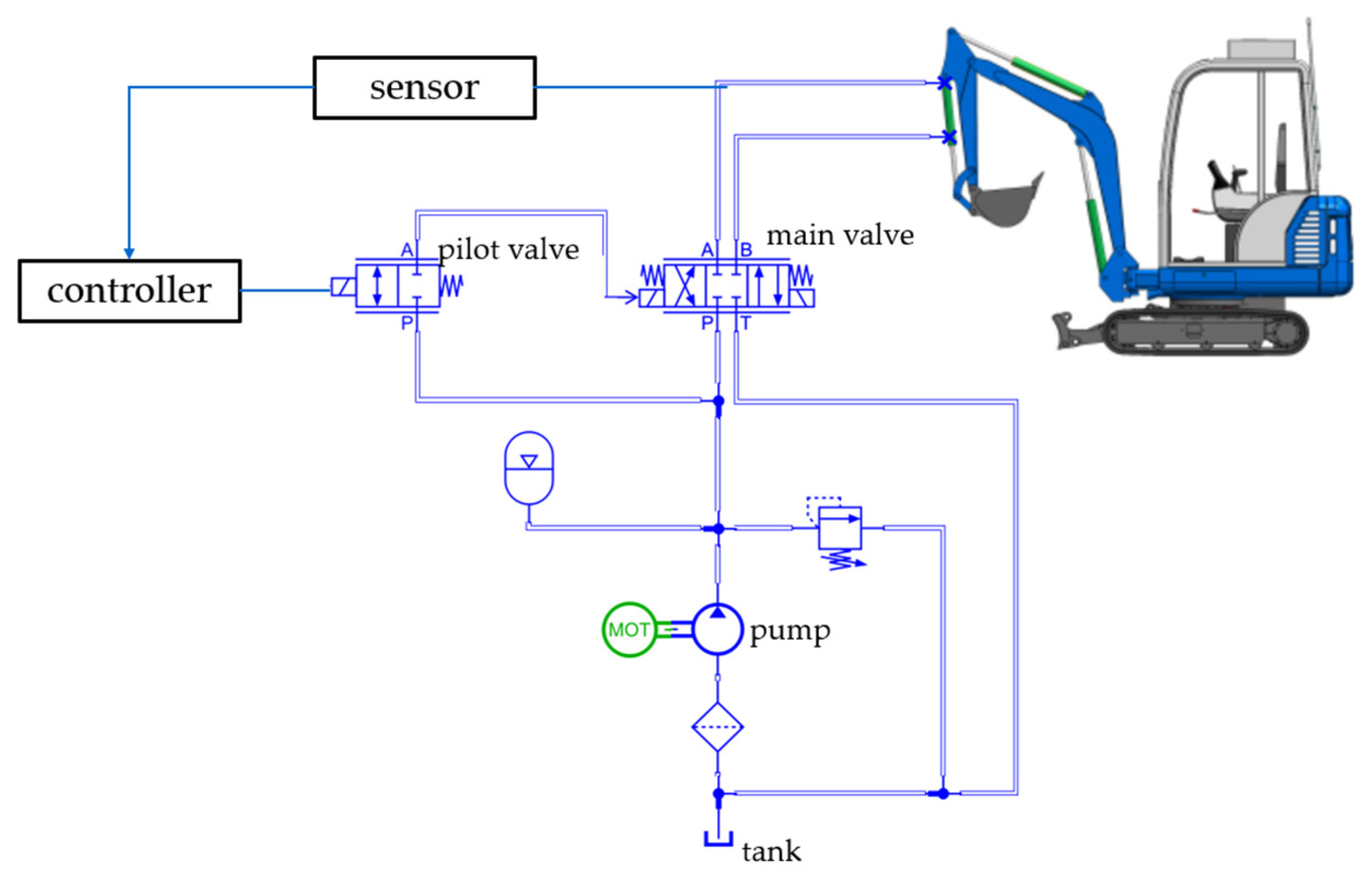
Figure 1. Structure of the electro-hydraulic control system.
Processes 11 01918 g001
Figure 2. D-H coordinates.
Processes 11 01918 g002
Figure 3. Input and response of system identification: (a) Input signal; (b) response.
Processes 11 01918 g003
Figure 4. Comparison between model and real system: (a) Input signal; (b) response.
Processes 11 01918 g004
Figure 5. Structure of ANMPC.
Processes 11 01918 g005
Figure 6. Experiment platform.
Processes 11 01918 g006
Figure 7. Desired bucket tip trajectory: (a) In X-Z plane; (b) X-axis; (c) Z-axis; (d) bucket angle.
Processes 11 01918 g007
Figure 8. Desired joint trajectory: (a) Boom; (b) arm; (c) bucket.
Processes 11 01918 g008
Figure 9. Tracking result and errors of boom: (a) Trajectory; (b) errors.
Processes 11 01918 g009
Figure 10. Tracking result and errors of Arm: (a) Trajectory; (b) errors.
Processes 11 01918 g010
Figure 11. Tracking result and errors of bucket: (a) Trajectory; (b) errors.
Processes 11 01918 g011
Figure 12. Bucket tip trajectory and errors: (a) Trajectory; (b) errors.
Processes 11 01918 g012
Figure 13. Bucket tip in X-axis and errors: (a) Trajectory; (b) errors.
Processes 11 01918 g013
Figure 14. Bucket tip in Z-axis and errors: (a) Trajectory; (b) errors.
Processes 11 01918 g014
Figure 15. Bucket angle and errors: (a) Angle trajectory; (b) errors.
Processes 11 01918 g015
Table 1. The parameters of D-H coordinates.
Joint i   a i   ( m )   d i   ( m )   α i   ( ° )   θ i   ( ° )
1 (Rotation)0.650.8290−180 to 180
2 (Boom)1.800−56.1 to 65.5
3 (Arm)0.9500−30.0 to −154.0
4 (Bucket)0.53500−44.5 to −118.5
Table 2. The estimated parameters.
Parameters   a 1   a 2   a 3   a 4   a 5   a 6   a 7
Estimated Values0133.751.65 × 10−612.51.05 × 101081.331.047 × 104
Table 3. The estimated parameters of boom and arm.
Parameters   a 1   a 2   a 3   a 4   a 5   a 6   a 7
Boom053.32.5 × 10−55.01.05 × 101063.168.21 × 103
Arm089.173.67 × 10−58.331.05 × 101071.779.33 × 103
Table 4. Controller parameters.
ParametersBoomArmBucket
[ N p , N m ][10, 2][10, 2][10, 2]
[ u m i n , u m a x ] (mA)[−1000, 1000][−1000, 1000][−1000, 1000]
[ Δ u m i n , Δ u m a x ] (mA)[−100, 100][−100, 100][−100, 100]
[ y m i n , y m a x ] (m)[0, 0.38][0, 0.445][0, 0.352]
[ y ˙ m i n , y ˙ m a x ] (m/s)[−0.3, 0.3][−0.5, 0.5][−0.5, 0.5]
[ p m i n , p m a x ] (MPa)[−15, 15][−12, 12][−12, 12]
Dead zone (mA)[300, 300][220, 220][200, 200]
Table 5. Tracking errors of the experiment.
Errors (10−3 m)Joint SpaceCartesian Space
BoomArmBucketDistanceX-AxisZ-AxisAngle
LMPCMax4.13.926.487.525.663.90.0659
RMSE2.32.16.731.419.724.50.0425
ANMPCMax1.91.72.123.113.818.50.02
RMSE1.00.91.211.65.610.10.0083
Disclaimer/Publisher’s Note: The statements, opinions and data contained in all publications are solely those of the individual author(s) and contributor(s) and not of MDPI and/or the editor(s). MDPI and/or the editor(s) disclaim responsibility for any injury to people or property resulting from any ideas, methods, instructions or products referred to in the content.