Article

A Novel Cellular Network Traffic Prediction Algorithm Based on Graph Convolution Neural Networks and Long Short-Term Memory through Extraction of Spatial-Temporal Characteristics

1
College of Electronic and Information Engineering, Shandong University of Science and Technology, Qingdao 266590, China
2
School of Computing and Mathematical Sciences, University of Leicester, Leicester LE1 7RH, UK
*
Author to whom correspondence should be addressed.
Processes 2023, 11(8), 2257; https://doi.org/10.3390/pr11082257
Submission received: 16 June 2023 / Revised: 24 July 2023 / Accepted: 24 July 2023 / Published: 26 July 2023

Abstract

:
In recent years, cellular communication systems have continued to develop in the direction of intelligence. The demand for cellular networks is increasing as they meet the public’s pursuit of a better life. Accurate prediction of cellular network traffic can help operators avoid wasting resources and improve management efficiency. Traditional prediction methods can no longer perfectly cope with the highly complex spatiotemporal relationships of the current cellular networks, and prediction methods based on deep learning are constantly growing. In this paper, a spatial-temporal parallel prediction model based on graph convolution combined with long and short-term memory networks (STP-GLN) is proposed to effectively capture spatial-temporal characteristics and to obtain accurate prediction results. STP-GLN is mainly composed of a spatial module and temporal module. Among them, the spatial module designs dynamic graph data based on the principle of spatial distance and spatial correlation. It uses a graph convolutional neural network to learn the spatial characteristics of cellular network graph data. The temporal module uses three time series based on the principle of temporal proximity and temporal periodicity. It uses three long and short-term memory networks to learn the temporal characteristics of three time series of cellular network data. Finally, the results learned from the two modules are fused with different weights to obtain the final prediction results. The mean absolute error (MAE), root mean square error (RMSE), and R-squared (R2) are used as the performance evaluation metrics of the model in this paper. The experimental results show that STP-GLN can more effectively capture the spatiotemporal characteristics of cellular network data; compared with the most advanced model in the comparison model on the real cellular traffic dataset in one cell, the RMSE can be improved about 81.7%, the MAE is improved about 82.7%, and the R2 is improved about 2.2%.

1. Introduction

With the explosive development of the Internet and the widespread use of mobile terminals, total Internet access has grown exponentially. Cellular network communications have appeared in all aspects of people’s lives, brought great convenience, and met the need for a better material life and spiritual life [1]. What follows is that a huge amount of cellular network traffic data will be generated by users all the time [2]. Operators are caught off guard by the countless amounts of cellular network traffic data and rising user demand. Accurate cellular network traffic prediction can help mobile operators predict overall network usage and make appropriate resource allocations based on this prediction, helping them improve network resource utilization and avoid resource waste [3]. In addition, accurate cellular network traffic prediction can improve the user experience and enable operators to dynamically adjust the base station usage in hotspot areas and times of day to avoid network congestion, so that users can enjoy the most appropriate services anytime, anywhere [4,5].
Therefore, cellular traffic prediction is an indispensable research field, but it is a challenging problem [6]. For now, the main difficulty of cellular network traffic prediction is the complex spatiotemporal characteristics. Cellular network traffic data are a kind of temporal sequential data, but the mobility of cellular network users is constantly convenient and fast, which makes the traffic values in different regions have cross-space characteristics, which increases the complexity of data characteristics. Secondly, traditional forecasting methods can only deal with simple temporal data and cannot deal with high complexity data with concurrent temporal and spatial characteristics. In addition, traditional methods also need to satisfy fixed assumptions, but in real life, highly complex data does not fit the ideal assumptions. In this case, a novel algorithm is needed to deal with highly complex data and make sure the two characteristics do not interfere with each other.
In summary, the challenges and problems in cellular network traffic prediction mainly include the following points: Firstly, how to exact and make full use of the spatial-temporal characteristics of cellular network traffic data? Secondly, how to avoid the influence of other characteristics when capturing one? Finally, which network structure is applied to meet the above two conditions and obtain accurately predicted values? To solve the above problems, this paper proposes a spatial-temporal parallel prediction model based on graph convolution combined with long and short-term memory networks (STP-GLN) for predicting cellular network traffic, which can model temporal dependence and spatial dependence, respectively. The main contributions of this paper are summarized as follows.
  • We build the cellular network on graphs based on the principle of spatial correlation between cells within the same period. The Pearson correlation coefficient is used to calculate the correlation between all cells at the time step t-th. The Euclidean distance is used to calculate the spatial distance between all cells. The spatial correlation is represented by the two together to construct the adjacency matrix so that the cellular network is built on a graph for each time step. Thus, the spatial graph of the cellular network is different for each time step.
  • We build the cellular network on time series based on the principles of temporal proximity and periodicity. The hourly sequence, daily sequence, and weekly sequence of each time step t-th are calculated by using the principles of proximity and periodicity, and then all moments are combined together to obtain the final hourly sequence, daily sequence, and weekly sequence.
  • A spatial-temporal parallel module is proposed to consider both spatial and temporal characteristics. The graph convolution neural (GCN) network module is used to learn the spatial characteristics of the graph data, and the long short-term memory (LSTM) module is used to learn the temporal characteristics of three kinds of time series. The input and output between modules do not affect each other. This allows us to capture spatial and temporal dependencies more realistically and effectively.
  • Simulation experiments are carried out on real data sets and compared with other models. The experimental results show that our model has better prediction results.
This paper is divided into five sections, and the rest of the structure is as follows. In Section 2, we describe the relevant parts. In Section 3, we present the source of the dataset, detailed data pre-processing, and analysis of the data. In Section 4, we explain how spatial graph data, three types of time series data are constructed, and the network structure of the prediction model. In Section 5, the experimental results are presented, compared, and analyzed. In Section 6, the paper is summarized.

2. Related Work

Network traffic data are essentially time series data [7]. Therefore, in the initial stage, the network prediction problem was only built on the time axis. The forecasting methods only predict the future change trend according to the past traffic change law and use the differences between traffic values at different moments as a quantification of traffic growth potential [8]. For example, Historical Averaging (HA) takes the average of the flow value in the past period as the flow value in the next moment. Linear Prediction [9], the Auto Regression Integrated Moving Average Model (ARIMA) model [10,11], and the Seasonal Auto Regression Integrated Moving Average Model (SARIMA) [12,13] are classical forecasting methods that usually have complete theoretical support and a good performance in time series with obvious periodicity and smoothness. However, with the strengthening of end-user mobility, network traffic data also has a certain degree of regular distribution in space, the traditional linear time series methods only analyze the characteristics of traffic data on the time axis, which can no longer obtain accurate prediction results. Artificial intelligence methods can extract various characteristics of the dataset well. The deep learning methods belonging to artificial intelligence have strong learning ability, which can extract the most useful characteristics from the complex dataset and learn the regularity and randomness of the data. For nonlinear time series data, deep learning can learn the temporal and spatial characteristics well and obtain accurate prediction results. Therefore, the prediction methods based on deep learning have become a hot spot in the research of cellular network traffic prediction.
In recent years, machine learning/deep learning methods have received widespread attention because of good fitting ability, inference ability, and expression ability. They have been applied to various fields [14]. Many researchers also use machine learning/deep learning as technical tools to study cellular network traffic prediction problems. Among this, Zhang, L. et al. [15] proposed a model based on Support Vector Machine (SVM) for multi-step traffic flow prediction. SVM can find the optimal hyperplane after finding the data regularity, but there is no general solution to the nonlinear problem, and sometimes it is difficult to find a suitable kernel function. Awan, F. M. et al. [16] used noise pollution data to make smart city traffic prediction based on LSTM. Fu, R. et al. [17] used LSTM and gated recurrent unit (GRU) for short-term traffic flow prediction. LSTM and GRU can obtain the time series characteristics of traffic data well but did not consider the impact of other factors on cellular network traffic data. Zhang, C. et al. [18] proposed a neural network model STDenseNet. It used densely connected convolutional neural networks (CNN) [19] to design two networks with shared structure, one for learning temporal proximity, and one for learning temporal periodicity. Daoud, N. et al. [20] used LSTM, CNN-LSTM, and ConvLSTM, three neural network models, to predict the global dust zone aerosol optical depth (AOD). Since CNN has an excellent performance capturing spatial characteristics, STDenseNet was also learning spatial characteristics while learning temporal characteristics. However, CNN is more suitable for extracting spatial characteristics than temporal characteristics, while LSTM is more suitable for extracting temporal characteristics. CNN is limited to characterizing grid-based traffic data [21,22]. The CNN for traffic prediction is more suitable for Euclidean structures and cannot be easily applied to non-Euclidean structures, but, in reality, most of the traffic data belong to non-Euclidean data.
Guo, K. et al. [23] proposed a graph convolutional recurrent neural network model named OGCRNN for traffic prediction, using the Graph Convolution Gated Recurrent Unit (GCGRU) [24] to learn the spatial-temporal characteristics of traffic data. GCN can be used for non-Euclidean structures, which is more realistic. Yu, B. et al. [25] proposed a neural network model named STGCN. It constructed traffic networks on graphs and proposed spatial-temporal GCN that used two graph convolution algorithms, Chebyshev Polynomials Approximation [26,27] and 1st-order Approximation [28], to process the spatial characteristics of traffic networks. GRU was used in temporal layers to process the temporal characteristics of the traffic network, and the accuracy is significantly improved. The spatial-temporal module in STGCN was a “sandwich” structure, where two temporal layers are sandwiched by a spatial layer. The input of the spatial layer is the output of the temporal layer plus the adjacency matrix, but the output generated by the temporal layer cannot fully represent the pattern of the original transportation network data, and the original data pattern may change through complex temporal layer operations. OGCRNN [23] and STGCN [25] were used for spatial-temporal characteristics of traffic data, but not for spatial-temporal characteristics of cellular data [29].

3. Datasets

3.1. Data Sources

In 2014, Telecom Italia together with MIT Media Lab, and other institutions jointly launched the “Telecom Italia Big Data Challenge” [30], which includes electricity data, telecommunications data, social network data, and more for the city of Milan and the province of Trentino (https://dataverse.harvard.edu/dataverse/bigdatachallenge, accessed on 6 April 2022). This paper uses the telecommunications data portion of the dataset for the city of Milan, which records 62 days of cellular network data from 0:00 on 1 November 2013 to 0:00 on 1 January 2014. Table 1 lists the dataset information.
As shown in Figure 1, in order to have a uniform operation when using the dataset, this dataset divides the city of Milan into M × N areas of M rows and N columns. Each area with a size of 235   m × 235   m , and this paper refers to an area of this size as a cell. In the actual data set, both M and N are 100. The grid division is designed according to the WGS84 coordinate system.
Each cell records five types of cellular network data at a time granularity of 10 min, i.e., all data of the five types generated are recorded and stored every 10 min in each cell, and the five types of cellular data recorded by each cell are:
  • (SMS-in) Number of SMS messages received within the cell: If any user receives an SMS message in any cell, a record of the SMS message reception service will be generated for that cell;
  • (SMS-out) Number of SMS messages sent within the cell: If any user sends an SMS message in any cell, a record of the SMS message sending service will be generated for that cell;
  • (Call-in) Number of Call messages received within the cell: If any user receives a call message in any cell, a record of the incoming call message will be generated for that cell;
  • (Call-out) Number of outgoing Call messages within the cell: If any user issues a call message in any cell, a record of the outgoing call message will be generated for that cell;
  • (Internet) Wireless network traffic data within the cell: If any user initiates an Internet connection or ends an Internet connection in any cell, a record of wireless network traffic data services will be generated for that cell. A record will also be generated if the connection lasts longer than 15 min or if the user transmits more than 5 MB during the same connection.

3.2. Data Pre-Processing

As shown in Figure 2, the data pre-processing in this paper mainly has the following three steps.
  • Data aggregation. The original dataset collected data at a 10 min aggregate granularity, which resulted in many cells having sparse cellular network data values, with mostly recorded values of 0. Therefore, this paper takes 1 h as the time granularity of statistics to ensure that most of the data have a value other than 0 and ensure the validity of the data.
  • Data filtering. The original dataset divided the city of Milan into 100 × 100 cells, from which we chose 20 × 20 cells as the dataset used in this paper. The cell IDs we chose are 4041–4060, 4141–4160……, 5941–5960.
  • Data normalization. In this paper, the data are processed by using the maximum–minimum normalization method and map its scale to the interval [0, 1]. Finally, when analyzing and comparing the experimental results in Section 5, the data are reversed to the original data range.

3.3. Data Analysis

3.3.1. Temporal Characterization

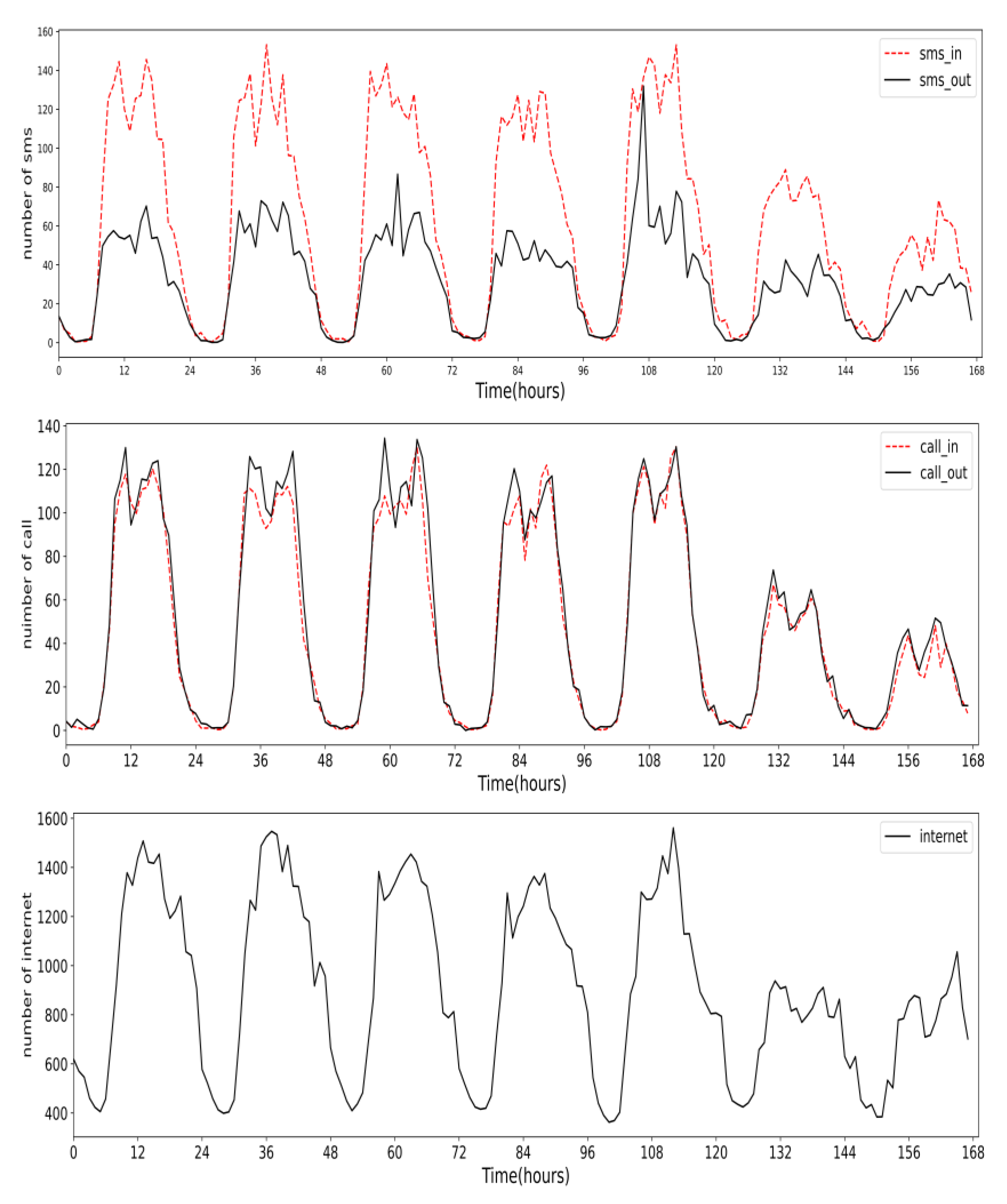
Figure 3 shows the trend of dynamic changes over time within five types of cellular network data in one cell over a given period of time. The X-axis represents the time, where we use 12 h as the interval unit and intercept a certain week in the dataset as the length of time. The Y-axis represents the number of events that occurred at a given time for a particular cellular network data type.
As can be seen from Figure 3, there is a disparity in the usage of the five types of cellular network data. The number of SMS messages received is significantly higher than the number of SMS messages sent. The number of incoming and outgoing calls is roughly the same. Wireless network traffic data usage is significantly higher than the number of SMS services and call services.
The dynamic change trends of five cellular network services in the temporal dimension are similar. They will show the same trend of change in the same time period, such as up or down. There is also a regularity in the amount of usage of the five services. For example, within a day, data usage is significantly higher during the day than at night; within a week, data usage is higher on working days than on weekends. The temporal characteristics have proximity; the data usage of adjacent periods in a day is similar, for example, the data usage at 15:00 on Monday is similar to that at 16:00 on Monday. Temporal characteristics also have periodicity: Every week from Monday to Friday there is a periodicity in the unit of days, which is the daily periodicity, but the daily periodicity in working days is different from the daily periodicity on weekends. Each month, there is a periodicity in the unit of weeks, which is the weekly periodicity. The data usage of the adjacent weeks is similar.

3.3.2. Spatial Characterization

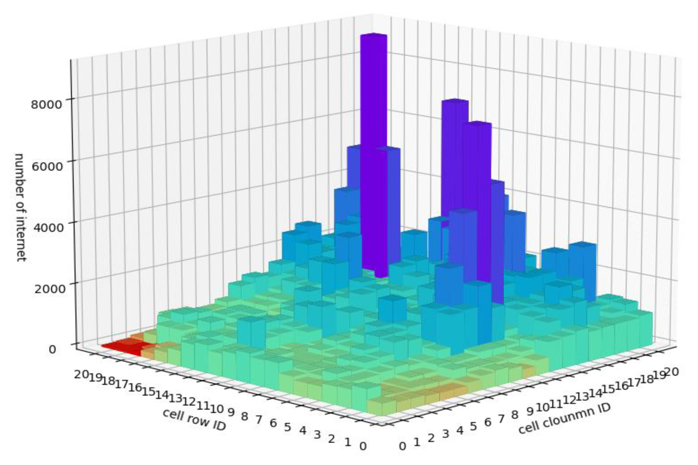
This section takes wireless network traffic data as an example and selects the usage of wireless network traffic data in Milan during the period from 03:00 to 04:00 on 1 November 2013 to analyze the spatial characteristics of wireless service traffic.
As shown in Figure 4, we show the usage of wireless traffic data in all cells at a certain time period. Different colors in Figure 4 represent different sizes of wireless network traffic data values. For example, red represents smaller values, and purple represents larger data values. It can be concluded that the usage of wireless traffic data is unevenly distributed among different cells. The usage of wireless traffic data in the densely populated urban center is higher than that in the sparsely populated urban edge. Therefore, the place with the maximum value means that the usage rate of wireless traffic in this area is high and it belongs to the urban central area. The spatial difference of wireless traffic data is transitional, that is, the data usage of adjacent cells is similar, only when the spatial distribution of the two cells exceeds a certain distance, the usage will have a big difference. This shows that the spatial correlation of wireless service data between different cells depends on the spatial distance between cells to a certain extent.
In order to accurately characterize the magnitude of correlation of cellular network traffic data in the spatial dimension, this paper uses Pearson’s correlation coefficient to calculate the correlation of cellular network traffic data among all cells in the same time period and serves as one of the bases for the spatial correlation metric [31]. The principle is
ρ i j = c o v x i , x j σ x i σ x j
where c o v is the covariance and σ is the standard deviation; x i is the cellular traffic value of cell i , and x j is the cellular traffic value of cell j . The larger the absolute value of Pearson correlation coefficient is, the closer it is to 1 or −1, the greater the spatial correlation is, and vice versa, the smaller it is.
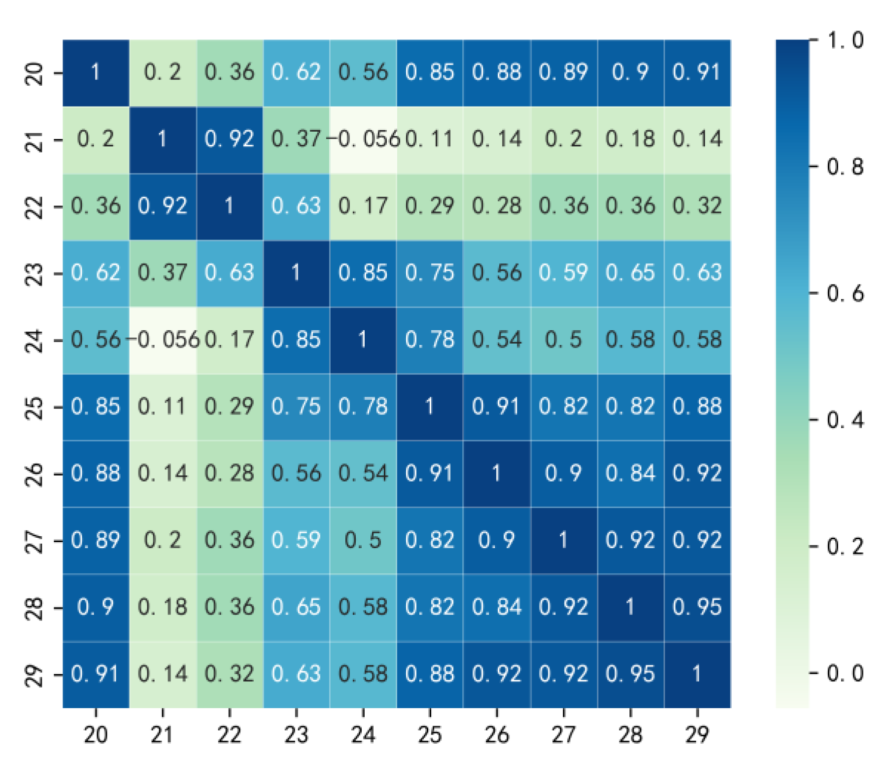
Here, the wireless network traffic data for all time between the 20-th cell and the 29-th cell is selected as an example. Figure 5 shows that, on the one hand, the wireless traffic volume values between adjacent cells are similar. For example, the distance between cell 24 and cell 25 is close, while the distance between cell 24 and cell 26 is slightly farther, so the spatial correlation between cell 24 and cell 25 is higher than that between cell 24 and cell 26. On the other hand, the correlation between cells with the same distance from the target cell is not necessarily equal, for example, cell 24 has the same spatial distance with cell 23 and cell 25, but the spatial correlation between cell 24 and cell 23 is higher than that between cell 24 and cell 25. Therefore, the spatial distribution of cellular data is regular. The smaller the spatial distance between two cells, the more similar the amount of data used by the two cells in the same period of time, the higher the spatial correlation. However, it is also variable. If there are two cells with the same spatial distance from the target cell, the spatial correlation between the two cells and the target cell may not be the same.
From the above, the spatial distribution of the amount of wireless network data used is correlated, to some extent distance dominates, but not all depends on distance. In this case, we should find a way as precise as possible to construct spatial correlation.

4. Data Construction and Forecast Model

Based on the analysis of the spatial-temporal characteristics of the data in Section 3, we describe how to construct graph data and three kinds of time series data, an hourly series, daily series, and weekly series, based on the pre-processed telecom data of Milan city, and then explain the model constructed according to the spatiotemporal characteristics.
The constructed spatiotemporal data better highlights the spatiotemporal characteristics, so that the deep-learning algorithms can find the regularity and randomness between the data more easily and obtain more accurate prediction results.

4.1. Graph Data Construction

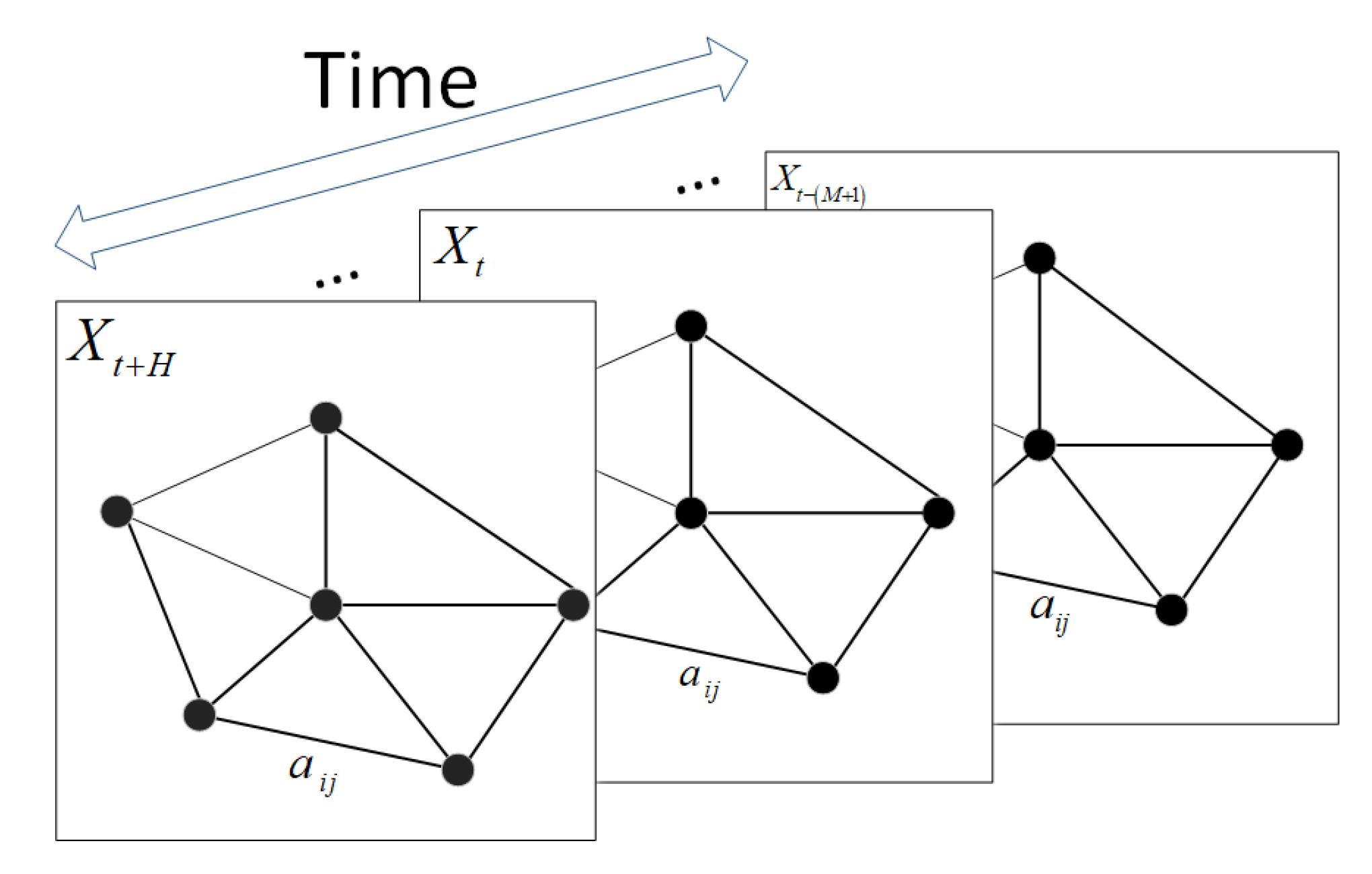
In this work, we use graphs to define the cellular network of the city of Milan. As shown in Figure 6, the cellular network of the city of Milan is defined as a graph G t = V t , E t , A t in chronological order at intervals for each time step t-th.
The city of Milan is divided into 20 × 20 cells; each cell i at time step t-th is represented as the node v t i on the graph, V t represents the set of all N nodes’ data at the time step t-th, V t = v t 1 , v t 2 , , v t n R N × 1 . E t is the set of edges at the time step t-th. A t R N × N are the adjacency matrices of the graph at time step t-th, A = A 1 , A 2 , , A T R T × N × N represents the set of adjacency matrices of at all moments T . The graph structure changes with time, and t = t Z | 0 t < 1488 .
In general, we can use the Euclidean distance between nodes to represent the spatial correlation between nodes, but from Figure 5, it can be concluded that the spatial distribution of cellular traffic data does not depend entirely on spatial distance. Therefore, we use the Pearson correlation coefficient and the Euclidean distance between each cell to construct the adjacency matrix A t at time step t-th. The Pearson coefficient is already expressed by Equation (1), the Pearson correlation between all cells at time step t-th can be represented via a matrix.
ρ t = ρ t 11 ρ t 1 j ρ t i 1 ρ t i j
The expression for the Euclidean distance between cell i and cell j is
d i j = r i r j 2 + c i c j 2
where r i is the row where cell i is located in 20 × 20 cells, and c i is the column where cell i is located in 20 × 20 cells. Similarly, r j is the row where cell j is located in 20 × 20 cells, and c j is the column where cell j is located in 20 × 20 cells. The spatial distance matrix D R N × N denotes
D = e d 11 2 e d 1 j 2 e d i 1 2 e d i j 2
Therefore, this paper constructs the adjacency matrix at time step t-th as
A t = 1 i = j ρ t D o t h e r s i z e
where is the Hadamard product.

4.2. Time Series Data Construction

Cellular traffic forecasting problems are essentially time series problems. We analyze and extract the characteristics of historical time series X H = X t T + 1 , , X t 1 , X t R N × T to predict the most likely cellular network data value X P = X t + 1 , , X t + H R N × H in the next H time steps.
Based on the above analysis of temporal characteristics in Section 3, we take into account the cellular traffic data of the n-th node at time step t-th, it is represented as x t n . Cellular traffic data for all nodes at time step t-th is expressed as X t = x t 1 , x t 2 , x t N R N × 1 . As shown in Figure 7, this paper divides the time series into three parts according to proximity and periodicity: hourly sequence, daily sequence, and weekly sequence.

4.2.1. Hourly Sequence X c

It consists of a sequence of cellular traffic data combined for Δ c hours before any time t . Take the cellular traffic data of Δ c hours before any time t to form the hourly data of each time, and the set of data at all time is the hourly sequence, that denotes
X c = X t c , X t ( c 1 ) , , X t 1 , X t
But there are some moments that do not have Δ c historical time steps, so there are requirements for any time t , t Δ c .

4.2.2. Daily Sequence X p

It consists of a sequence of cellular traffic data combined for Δ p × 24 hours before any time t . Take the cellular traffic data of Δ p × 24 hours before any time t to form the daily data of each time, and the set of data at all time is the daily sequence, that denotes
X p = X t p × 24 , X t ( p 1 ) × 24 , , X t 24 , X t
But there are some moments that do not have Δ p × 24 historical time steps, so there are requirements for any time t , t Δ p × 24 .

4.2.3. Weekly Sequence X w

It consists of a sequence of cellular traffic data combined for Δ w × 168 hours before any time t . Take the cellular traffic data of Δ w × 168 hours before any time t to form the weekly data of each time, and the set of data at all time is the weekly sequence, that denotes
X w = X t w × 168 , X t ( w 1 ) × 168 , , X t 168 , X t
But there are some moments that do not have Δ w × 168 historical time steps, so there are requirements for any time t , t Δ w × 168 .

4.3. Proposed Forecasting Model

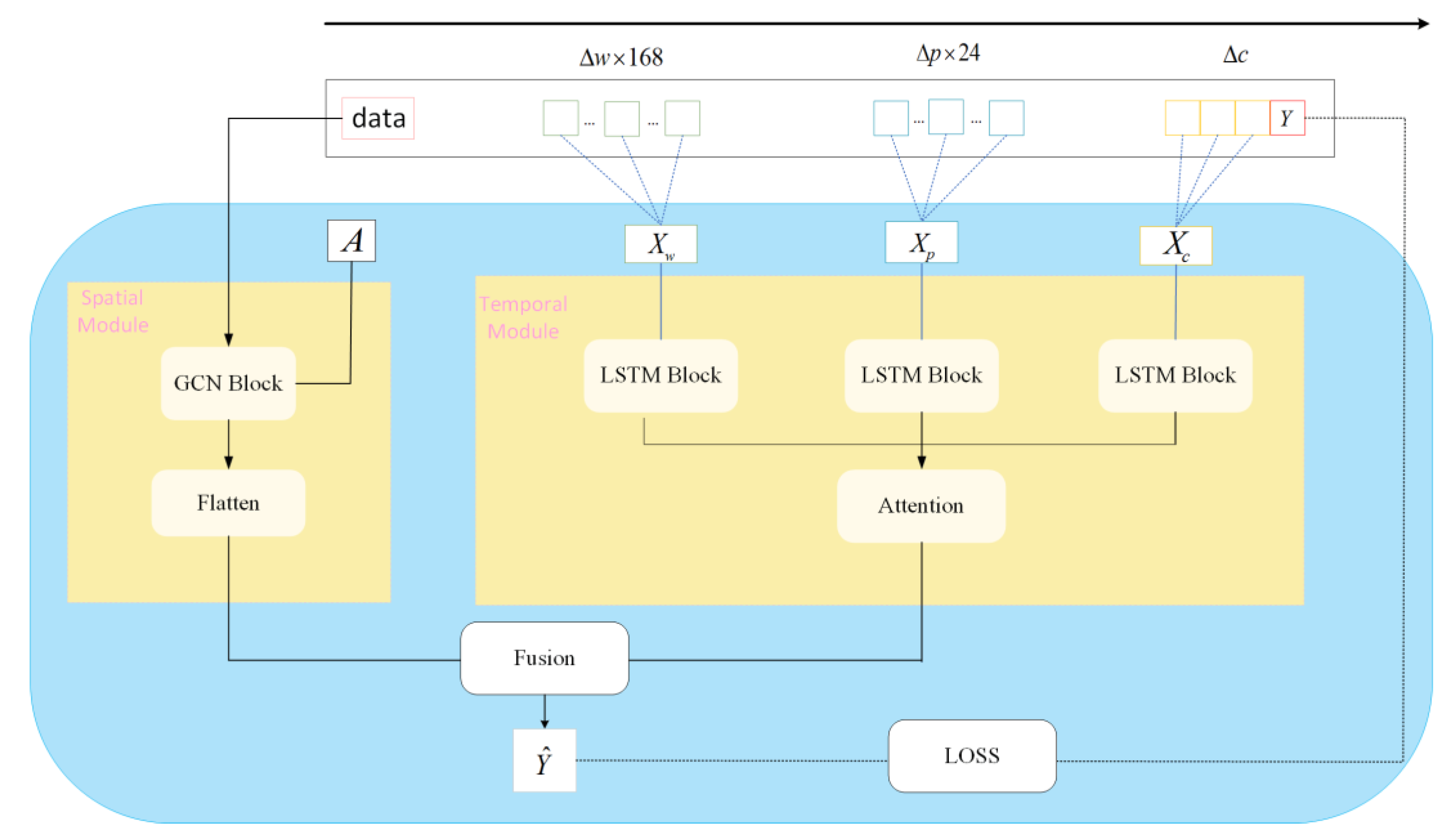
In this section, we elaborate on the proposed architecture of STP-GLN. As shown in Figure 8, the STP-GLN mainly consists of two parallel modules, one of which is a spatial module and a temporal module. The spatial module consists of spatial GCN blocks, and the temporal module consists of temporal LSTM network blocks. Details of each module are shown below.
According to the spatial-temporal characteristics, STP-GLN adopts different data input as support, and processes the original data into graph data form and three time sequence forms, giving full play to the maximum advantages of each module. STP-GLN uses two deep-learning algorithms to model the spatiotemporal dependencies. In the temporal module, three LSTM networks are used to model the adjacency and periodicity of the time dependence. In the spatial module, GCNs are used to capture the spatial dependence efficiently.

4.3.1. Graph Convolutional Neural Network Module

Previous studies have ignored the spatial nature of cellular networks [32], and while the datasets meshing the city of Milan are conducive to constructing graph data, they do not take into account spatial connectivity and the global nature. Even with two-dimensional convolution, they can only roughly capture spatial characterization. Therefore, in our model, graph convolution is used directly on graph structure data to extract highly meaningful spatial characterization.
In order to capture the spatial characteristics at different timestamps, the module captures the spatial characteristics of cellular network data through a two-layer graph convolutional neural network. Since the cellular network data graph is considered to be an undirected graph, we can use the first-order approximation method in spectral convolution to perform feature extraction on the nodes in the cellular network data graph [28].
Feature extraction of graph convolutional layers can be expressed as
Θ * g X g ( l ) θ 0 X g ( l ) + θ 1 2 λ max L I n X g ( l ) = θ 0 X g ( l ) θ 1 D 1 2 A D 1 2 X g ( l )
where X g l , A are the inputs to the layer of the graph convolutional, and 0 < l 2 ; I n is the identity matrix, L denotes the normalized Laplace matrix of the cellular network data graph, and λ m a x is the maximum eigenvalue of L . Equation (9) approximates λ m a x to 2, so the equation can transition to the second equal sign. The two kernel parameters θ 0 , θ 1 can be shared in the diagram, and for more efficient operation in practice, let θ 0 = θ 1 = θ , then Equation (9) can be simplified to
Θ * g X g ( l ) θ I n + D 1 2 A D 1 2 X g ( l ) = θ D ˜ 1 2   A ˜ D ˜ 1 2 X g ( l )
where A and D are renormalized by A ˜ = A + I n and D ˜ i i = j A ˜ i j , respectively.
Generalizing Equation (10) to a signal X g ( l ) R N × T × 1 , which has C input channels and F filters, as follows
X G ( l ) = D ˜ 1 2   A ˜ D ˜ 1 2 X g ( l ) Θ
where Θ R N o n e × N × N is now the filter parameter matrix, and X G ( l ) R T × N is the convolutional signal matrix.
Each graph convolutional layer comes with a nonlinear R e L U · activation function, so the output of the l t h layer denotes
X R G C N l = R e L U X G l
In order to ensure the successful transition from the graph convolutional layer to the dense layer, a Flatten layer is added at the end of the spatial module to change the dimension of the output to one dimension. The output of the graph convolutional layer of the last layer is represented as X R G C N , so the output of the Flatten layer can be represented as
Y S = F l a t t e n X R G C N

4.3.2. Long Short-Term Memory Network Module

Although RNN-based models are widely used in time series analysis, RNN suffers from gradient explosions, which makes it impossible to correlate between inputs over a long period of time when backpropagating to adjust parameters. LSTM can alleviate the problems of RNNs in long-term sequences and make recurrent neural networks have stronger and better memory performance [33].
From the perspective of time characteristics, the changing trend of cellular network has the characteristics of long time series, non-linearity, adjacency, and periodicity. This section takes into account these characteristics to use LSTM to learn time characteristics from historical time series.
Combined with the learning process of LSTM, the feature extraction of three time series by the long short-term memory network can be expressed as
i t = σ W i X ( l ) + U i h t 1 + b i
f t = σ W f X ( l ) + U f h t 1 + b f
o t = σ W o X ( l ) + U o h t 1 + b o
C ˜ t = tanh W c X ( l ) + U c h t 1 + b c
C t = i t C ˜ t + f t C t 1
h t = o t t a n h C t
where i t , f t , o t correspond to input gates, forget gates, and output gates. X l represents the input of any time sequence of X C , X P , X W , and 0 < l 2 . C t 1 represents the state at the previous time. C ˜ t is the new variable generated by the t a n h ( ) function. C t represents the state at the current time t . C t 1 represents the state at the previous time t 1 . h t 1 represents the output at the previous time t 1 . h t represents the output at the current time t . W τ and U τ represent the weight parameters. b τ represents bias vectors, W τ , U τ , b τ are learnable parameters, τ { i , f , o , c } .
Each LSTM layer also comes with a R e L U activation function, so the output of the l-th layer denotes
Y R L S T M l = R e L U h t
Finally, the attention mechanism assigns different weights to the three time series features, forming the output of the final long and short-term memory network the output Y T . Luong-style attention [34] has been chosen as a measure of the importance of different time series.

4.3.3. Output Block

The purpose of this block is to integrate the output of the Graph convolutional neural network module and the Long short-term memory network module, and the impact of the two modules on each cell is different, so we define the output module as follows
Y ^ = W S , T ( Y s Y T )
where W S , T = W S , W T is a weight vector, and W S , T is learnable parameters.

4.3.4. Loss Function

In this paper, the mean squared error (MSE) is selected as the Loss function, and the proposed STP-GLN model is trained to obtain the predicted value, and the loss function can be written as
M S E = 1 n i = 0 n y ^ t i y t i 2
where y t i represents the i-th ground truth at time step t-th, y ^ t i represents the i-th forecasted value at time step t-th, and n represents the number of samples. Our model uses Adam’s algorithm to minimize the root mean square error (RMSE) loss for parameter updating [35,36].

5. Experiment and Evaluation

5.1. Training Paraments

STP-GLN trains 50 epochs with a batch size of 32 and a learning rate set to 0.001, optimized using Adam optimization techniques and R e L U as an activation function. We use 44 days as a historical time window, which uses 1056 data points to predict cellular traffic data for the next 264 h. During the training process, 80% of the entire dataset is randomly selected as the training set and 20% of the data is used as the test set. In total, 20% of the training set was randomly selected as the validation set. The model parameters are also shown in Table 2.

5.2. Performance Evaluation Method

In this paper, MAE, RMSE, and R2 are selected as evaluation indicators to measure the effectiveness of the proposed model and can be easily and quickly compared with other models, which are defined as follows
M A E = 1 n i = 0 n | y t i ^ y t i |
R M S E = 1 n i = 0 n y ^ t i y t i 2
R 2 = 1 i = 0 n y ^ t i y t i 2 i = 0 n y ¯ i y t i 2
where y t i represents the i-th node’s ground truth at time step t-th, y ^ t i represents the i-th node’s forecasted value at time step t-th, y ¯ i is the average of the i-th node and n represents the number of samples. The smaller the RMSE and MAE data values, the better the effect of the model. We briefly explain the three evaluation indicators:
  • RMSE reflects the degree of deviation between the ground truth and the forecasted value. The smaller its value, the better the quality of the model and the more accurate the prediction.
  • MAE evaluates the degree of deviation between the ground truth and the forecasted value, that is, the actual size of the prediction error. The smaller the value, the better the model quality and the more accurate the prediction.
  • R2 explains the variance score of the regression model, and its value takes the range of [0, 1]. The closer to 1 indicates the better the quality of the model and the more accurate the prediction, and the smaller the value, the worse the effect.

5.3. Results and Analysis

In order to verify the advantages of the proposed model, we show the comparison results of the actual and predicted values of STP-GLN in five types of data. The experimental results are shown in Figure 9, Figure 10, Figure 11. We also selected six time series prediction models to compare with our proposed models, namely HA, LR, GCN, LSTM, STDensenNet [18], and STGCN [25], among which HA has only one evaluation index in all communities. The experimental results are shown in Table 3, Table 4, Table 5.
In the selection of cells, we mainly choose two types of cells. The first one is all the cells in the test set, that is, the 264 moments of the true value of 400 cells compared with the predicted value. The second is the test set of the smallest error between the real value and the predicted value of one cell, that is, the 264 moments of the real value of one cell and the predicted value are compared, and the best cell predicted by the different models is not the same. Among which, HA is compared with other models only on the type of all cells. The experimental results are shown in Table 3, Table 4, Table 5.
The GCN and LSTM of the “Model” in Table 3, Table 4, Table 5 are the spatial model and the temporal module of the STP-GLN’s model, respectively. In order to clarify the role of each part of the STP-GLN model, we use three evaluation metrics to compare the correlation and importance of each module with the whole. As can be seen from Table 3 and Table 4, the spatial module plays a greater role than the temporal module in the SMS dataset and the Call dataset. From Table 5, it can be seen that in the Internet dataset, the temporal module plays a greater role than the spatial model. Moreover, as a whole, the prediction effect of STP-GLN is better than that of each module individually, which indicates that our model adopts the method of spatiotemporal parallel structure correctly and adopts two correct deep learning methods to learn spatiotemporal features separately.
Table 3, Table 4, Table 5 represent the results of comparing our model and other models using the evaluation metrics in the five categories of data, respectively. The valid data in Table 3, Table 4, Table 5 represent the results of comparing our model with other models. Meanwhile, because of the different order of magnitude of the five types of data, the usage of Internet is much larger than the usage of SMS and the usage of calls, and the usage of SMS is slightly larger than the usage of Call. Therefore, the prediction error in the Internet dataset is much larger than the prediction in the SMS dataset and the Call dataset, and the prediction error in the SMS dataset is larger than the prediction error in the Call dataset. This also explains why the valid numbers in Table 5 are greater than those in Table 3 and Table 4, and the valid numbers in Table 3 are greater than those in Table 4. Therefore, the effective numbers of the three tables can only be related to the datasets they use and not to the datasets in the other tables.
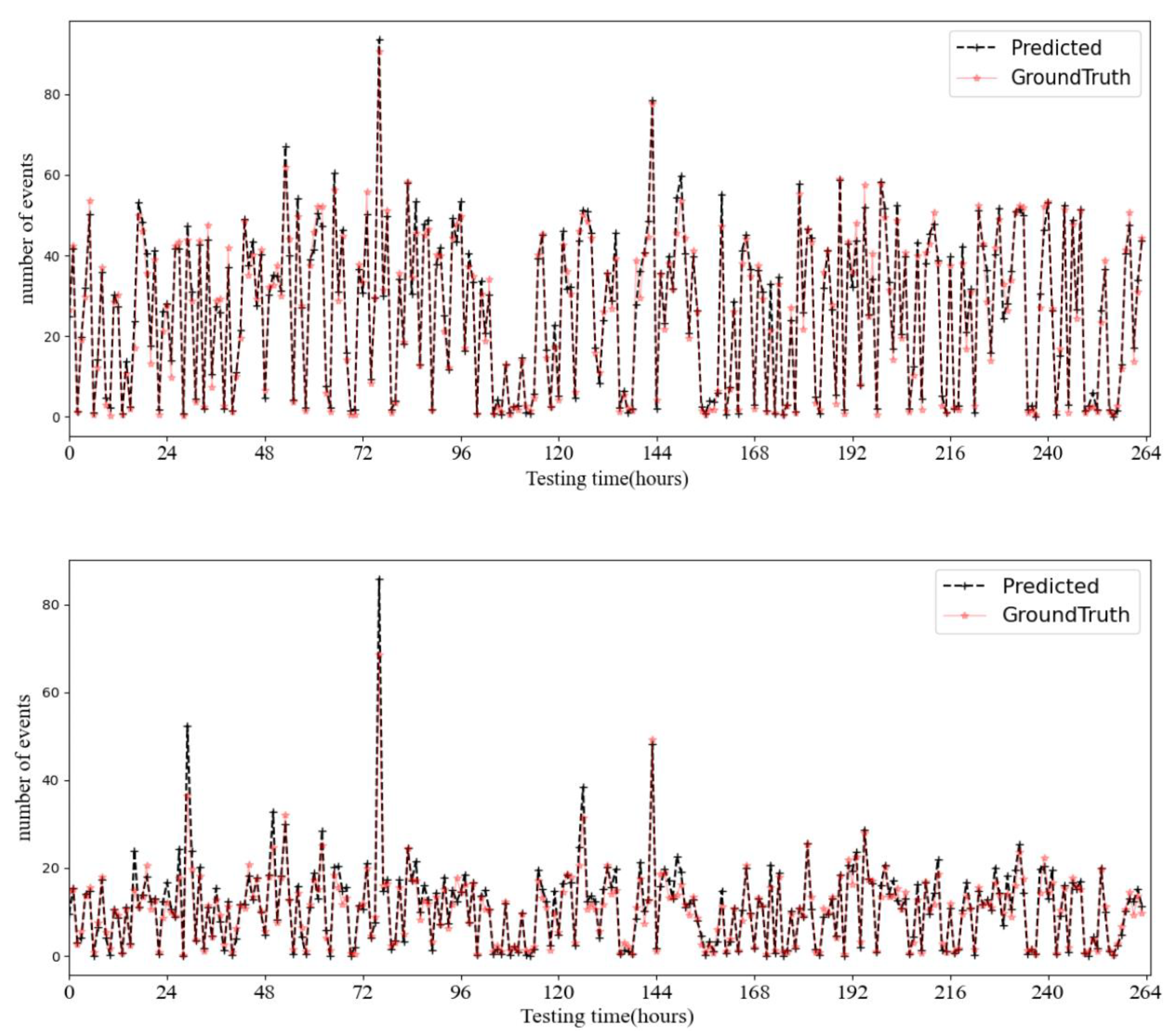
Figure 9 shows the comparison of prediction results for SMS dataset over 7 days in one cell. The above figure shows the comparison of prediction results of the receiving SMS (SMS-in) dataset in the test set, and the following figure shows the comparison of prediction results of sending SMS (SMS-out) dataset in the test set.
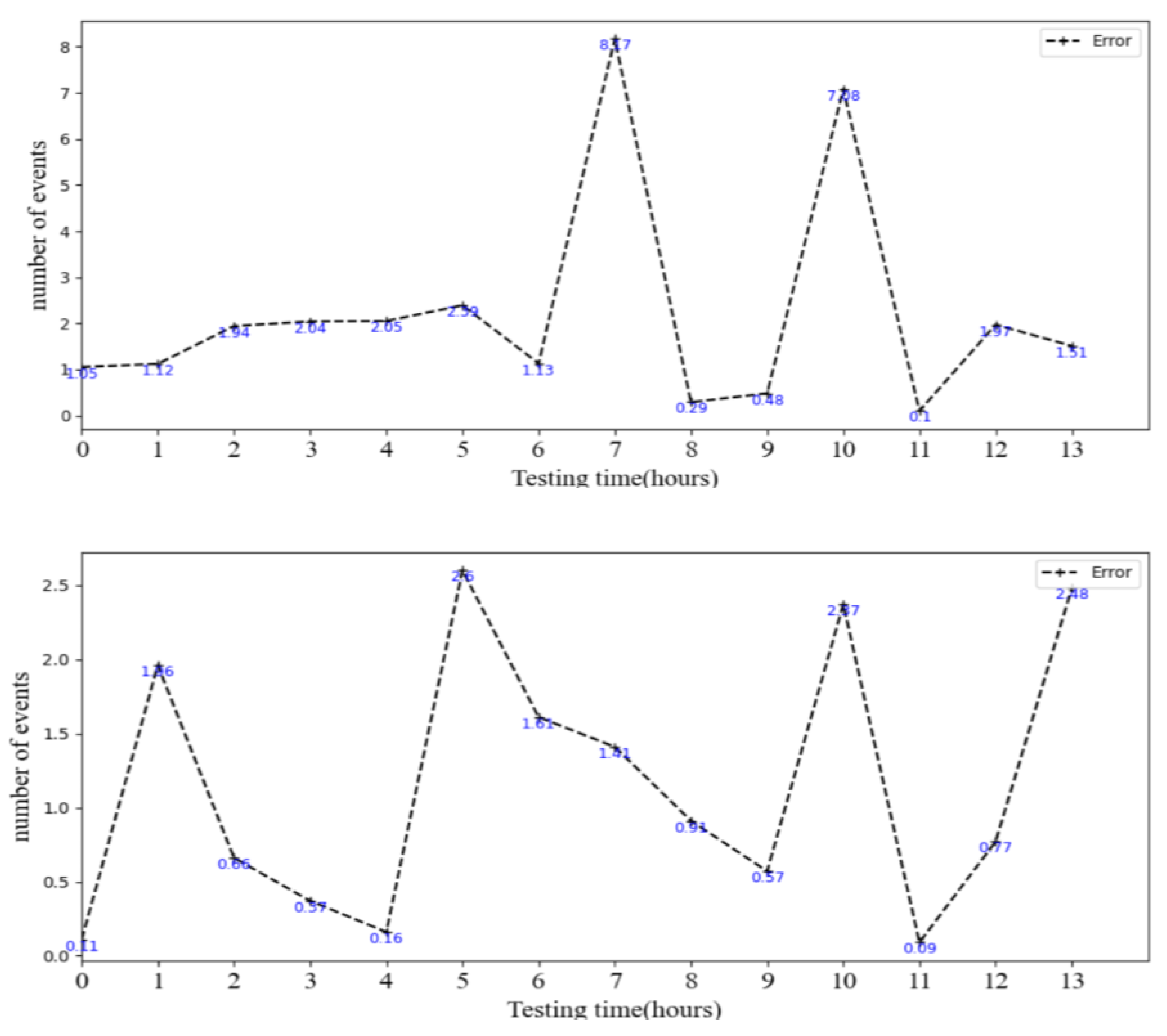
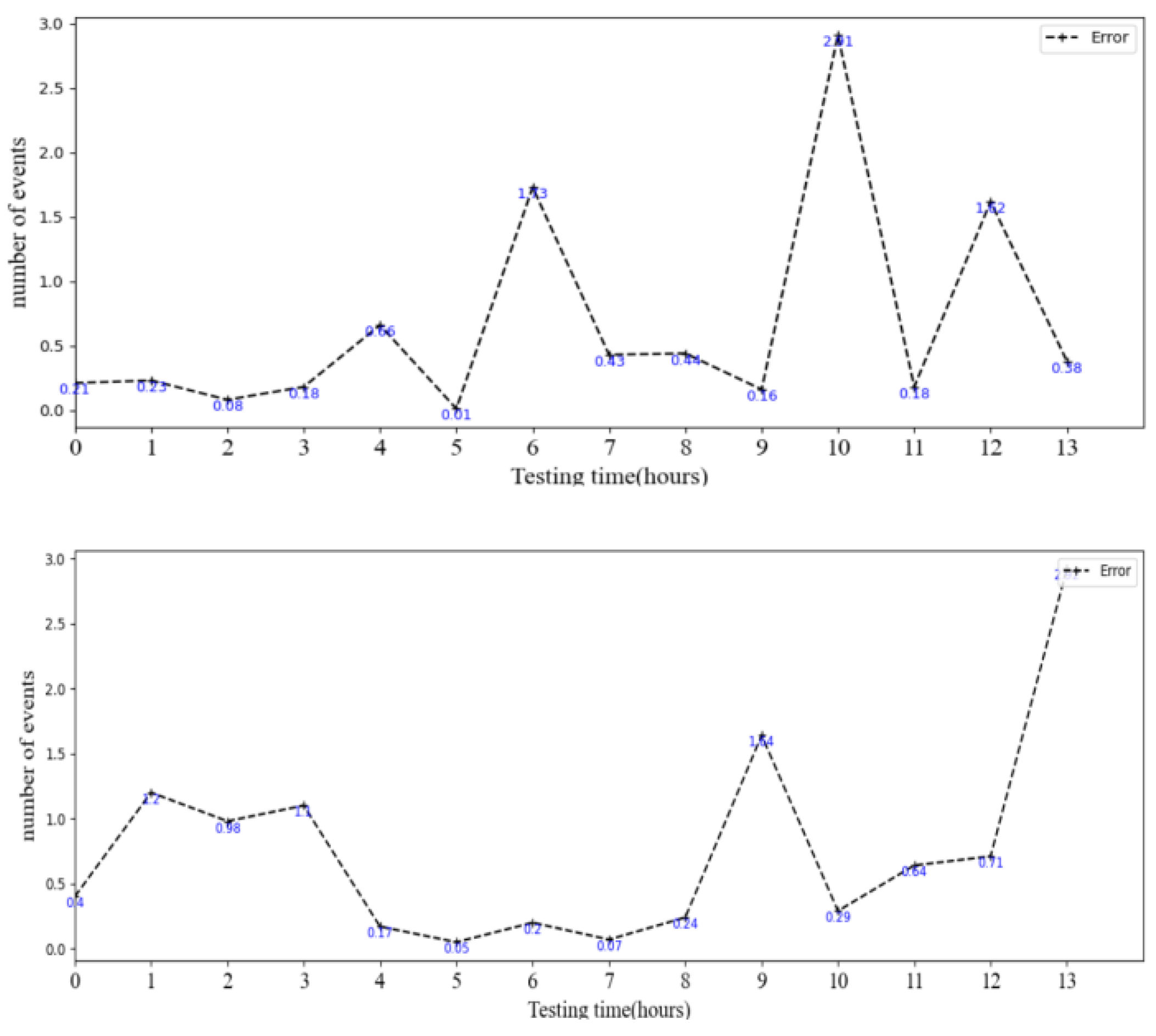
Figure 10 shows the absolute value of the error between the true and predicted values over a period of 14 h in one cell. The smaller the absolute value of the error in Figure 10, the better the prediction effect of the model. The above graph shows the prediction error for SMS-in dataset over a period of 14 h, the absolute error is at least 0.1 in this dataset, that is, the difference between the real value and the predicted value is 0.1, indicating that our model can well fit the future trend of the data. The following graph shows the prediction error for SMS-out dataset. The absolute error is at least 0.09, which indicates that the prediction effect is better.
The comparison of the experimental results of HA, LR, GCN, LSTM, STDensenNet [18], and STGCN [25] can be seen in Table 3. On the SMS dataset, our model is better than other models in the evaluation of three evaluation indicators. For example, compared to the state-of-the-art STGCN model in the model, RMSE improved the effect of the SMS-in dataset by 47.2% in one cell and 40.9% in all cells. MAE improved the effect by 52.6% in one cell and 30.5% in all cells. This indicates that the prediction error of our model is less than that of the other models, and R2 improved the effect by 7.8% in one cell and 22.9% in all cells, which indicates that the quality of our model is higher than that of the other models.
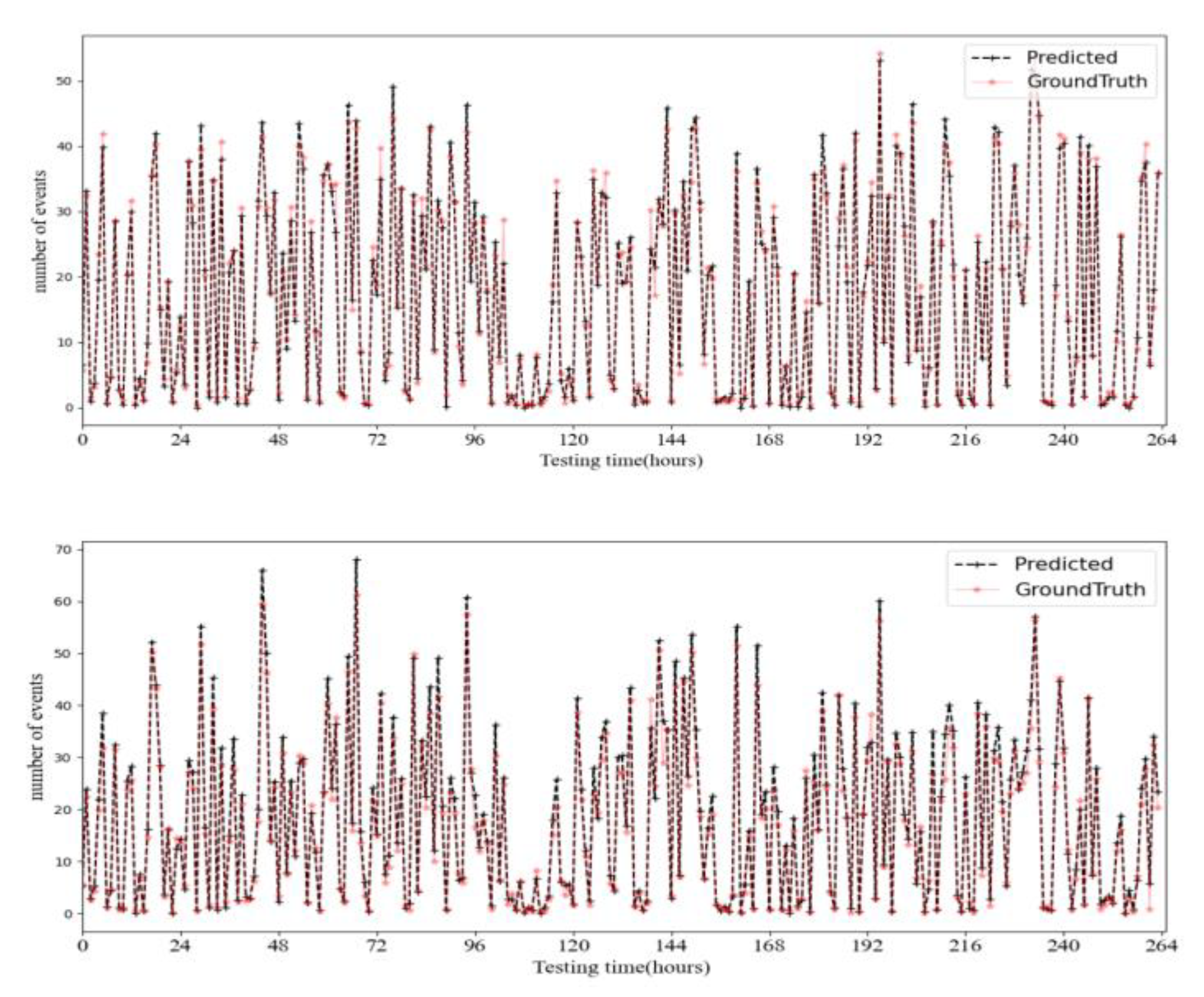
Figure 11 shows the comparison of the prediction results for Call dataset over 7 days in one cell. The above figure shows the comparison of prediction results of the incoming Call (Call-in) dataset in the test set, and the following figure shows the comparison of prediction results of outgoing Call (Call-out) dataset in the test set.
Figure 12 shows the absolute value of the error between the true and predicted values over a period of 14 h in one cell. The above graph shows the prediction error for Call-in dataset over a period of 14 h, and the following graph shows the prediction error for Call-out dataset. In the two subgraphs in Figure 12, the smallest absolute error is 0.01, which indicates that our model shows an accurate prediction in the Call dataset.
Table 4 compares the experimental results of HA, LR, GCN, LSTM, STDensenNet [18], and STGCN [25]. On the Call dataset, our model outperforms the other models in all three evaluation metrics measures. For example, compared to the state-of-the-art model STGCN, RMSE improved the effect of the Call-in dataset by 57.0% in one cell and 36.1% in all cells. MAE improved the effect by 53.4% in one cell and 31.2% in all cells. This indicates that the prediction error of our model is less than that of the other models, and R2 improved the effect by 4.7% in one cell and 9.3% in all cells, which indicates that the quality of our model is higher than the other models.
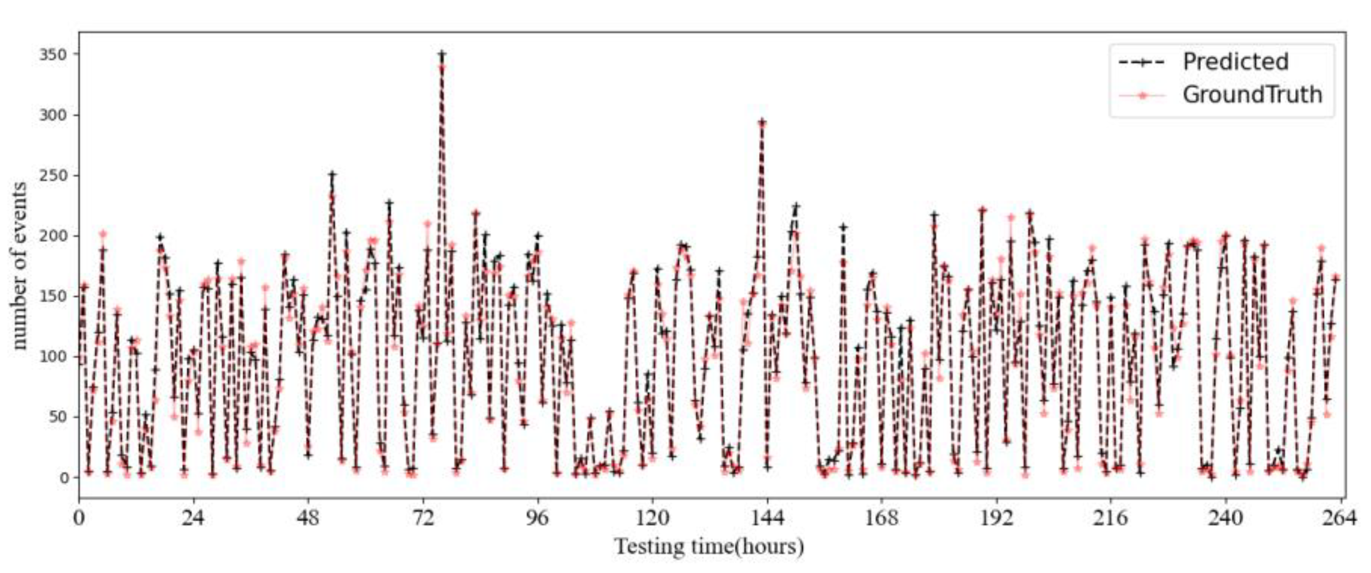
Figure 13 shows the comparison of prediction results for Internet dataset over 7 days in one cell. The figure shows the comparison of the prediction results of the Internet dataset in the test set.
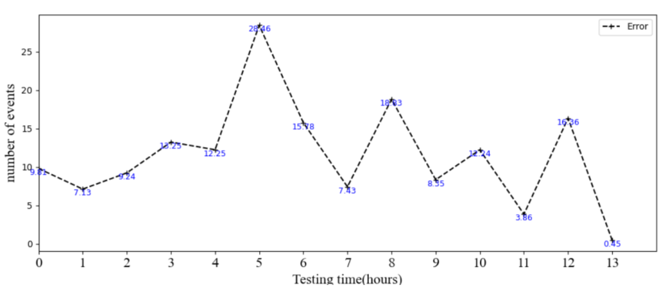
Figure 14 shows the absolute value of the error between the true and predicted values over a period of 14 h in one cell for internet dataset. The true value is measured in hundreds or thousands in this dataset, and our prediction error is controlled to within 30, which has little impact on the overall data.
Table 5 shows a comparison of the experimental results of HA, LR, GCN, LSTM, STDensenNet [18], and STGCN [25]. On the Internet dataset, our model outperforms the other models in all three evaluation metrics measures. For example, compared to the state-of-the-art model STGCN, RMSE improved the effect by 81.7% in one cell and 4.1% in all cells. MAE improved the effect by 82.7% in one cell and 12.7% in all cells. This indicates that the prediction error of our model is less than that of the other models, and R2 improved the effect by 2.2% in one cell and 7.6% in all cells, which indicates that the quality of our model is higher than that of the other models.
Figure 9, Figure 10, Figure 11 show the comparison of the prediction results of five types of data in one cell. These figures show the comparison of prediction results of short message service in the test set. The change trend of five types of data in Figure 9, Figure 10, Figure 11 is similar to that of the short message service under the spatial-temporal characteristics analysis in Section 3. The change trend of the predicted value is the same as that of the real value. Our model can well capture the peak value of the short message service. In general, the dynamic change curves of the two are basically consistent.
To verify the stability, novelty, and transferability of our model, we compared it with the STGCN model on the CIKM21-MPGAT dataset [37] in Table 6. From the comparison results, it can be seen that the prediction accuracy of our model is better than that of the STGCN model on the CIKM21-MPGAT dataset, which indicates that our model is not only accurate on the Milan dataset, but also has a good effect on other datasets, with good stability and novelty, and is transferable.
The results show that the proposed model has better prediction effect than the comparison model in the five types of data. The proposed model performs better in a single cell and in all the evaluation indicators of cells than the comparison model. We can also see that the forecasting results of traditional time series analysis methods are not ideal, which proves that the ability of these methods to process complex spatiotemporal data is limited. In contrast, deep learning-based methods generally obtain better forecasting results than traditional time series analysis methods. Among the single deep learning methods, the LSTM method and GCN method selected in this paper are the temporal module and the spatial module in the STP-GLN model, and the results show that the prediction method, using a deep-learning algorithm that only analyzes the temporal characteristics or the spatial characteristics, is better than the traditional method, but the prediction effect is less accurate than that of the model STP-GLN which also considers the spatiotemporal characteristics. It is shown that considering the spatiotemporal correlation of cellular networks is useful for data prediction in practice. In the deep learning method, the STDensNet model, the STGCN model, and the proposed model STP-GLN all take into account the spatiotemporal correlation, and it can be seen from the comparison results that the prediction effect of our model is better than the two comparison models.

6. Conclusions

In this paper, we propose a model STP-GLN based on two deep-learning algorithms to predict cellular network traffic. Cellular network traffic data for all cells in the city of Milan is constructed as graph-structured data and three time-series data. In constructing the adjacency matrix for the spatial module, we considered the spatial distance between nodes and the calculation of the Pearson correlation coefficient between all nodes at the same time t. Both of these methods, which can represent spatial correlation, are fused and together form the adjacency matrix. In constructing the temporal data, we arrange the data of all cells into hourly sequences, daily sequences, and weekly sequences according to the principles of nearest neighbors and periodicity, respectively. The dynamic spatiotemporal characteristics of the constructed spatial graph data and the temporal axis data are captured simultaneously using a graph convolutional neural network module and a long and short-term memory network module, respectively. Both our model and the comparison model are validated on a real dataset from the city of Milan, and the experimental results show that our model has improved prediction results for all five types of cellular network data compared to the state-of-the-art model in the comparison model. At the same time, our model is transferable, which can be used not only in the cellular data set mentioned in this paper but also in other cellular datasets; in addition, it can also be used in traffic volume forecasting, housing price forecasting, and other aspects.

Author Contributions

Conceptualization, G.C.; Data curation, Y.G.; Formal analysis, G.C. and Y.G.; Methodology, Q.Z.; Validation, Y.Z.; Writing—original draft, G.C.; Writing—review and editing, Y.G. All authors have read and agreed to the published version of the manuscript.

Funding

This research was funded by the National Natural Science Foundation of China under Grant No. 61701284, the Natural Science Foundation of Shandong Province of China under Grant No. ZR2022MF226, the Talented Young Teachers Training Program of Shandong University of Science and Technology under Grant No. BJ20221101, the Innovative Research Foundation of Qingdao under Grant No. 19-6-2-1-cg, the Elite Plan Project of Shandong University of Science and Technology under Grant No.skr21-3-B-048, the Hope Foundation for Cancer Research, UK under Grant No. RM60G0680, the Royal Society International Exchanges Cost Share Award, UK under Grant No. RP202G0230, the Medical Research Council Confidence in Concept Award, UK under Grant No. MC\_PC\_17171, the British Heart Foundation Accelerator Award, UK under Grant No. AA/18/3/34220, the Sino-UK Industrial Fund, UK under Grant No. RP202G0289, the Global Challenges Research Fund (GCRF), UK under Grant No. P202PF11. the Guangxi Key Laboratory of Trusted Software under Grant No. kx201901, the Sci. Tech. Development Fund of Shandong Province of China under Grant No. ZR202102230289, ZR202102250695 and ZR2019LZH001, the Humanities and Social Science Research Project of the Ministry of Education under Grant No. 18YJAZH017, the Taishan Scholar Program of Shandong Province under Grant No.ts20190936, the Shandong Chongqing Science and technology cooperation project under Grant No. cstc2020jscx-lyjsAX0008, the Sci. \& Tech. Development Fund of Qingdao under Grant No. 21-1-5-zlyj-1-zc, the SDUST Research Fund under Grant No. 2015TDJH102, and the Science and Technology Support Plan of Youth Innovation Team of Shandong higher School under Grant No. 2019KJN024.

Data Availability Statement

Data sharing not applicable.

Acknowledgments

The authors would like to extend their gratitude to the anonymous reviewers and the editors for their valuable and constructive comments, which have greatly improved the quality of this paper.

Conflicts of Interest

The authors declare no conflict of interest.

References

  1. He, Y.; Yang, Y.; Zhao, B.; Gao, Z.; Rui, L. Network Traffic Prediction Method Based on Multi-Channel Spatial-Temporal Graph Convolutional Networks. In Proceedings of the 2022 IEEE 14th International Conference on Advanced Infocomm Technology (ICAIT), Chongqing, China, 8–11 July 2022. [Google Scholar]
  2. Naboulsi, D.; Fiore, M.; Ribot, S.; Stanica, R. Large-Scale Mobile Traffic Analysis: A Survey. IEEE Commun. Surv. Tutor. 2016, 18, 124–161. [Google Scholar] [CrossRef] [Green Version]
  3. Zeng, Q.; Sun, Q.; Chen, G.; Duan, H.; Li, C.; Song, G. Traffic Prediction of Wireless Cellular Networks Based on Deep Transfer Learning and Cross-Domain Data. IEEE Access 2020, 8, 172387–172397. [Google Scholar] [CrossRef]
  4. Jiang, W. Cellular Traffic Prediction with Machine Learning: A Survey. Expert Syst. Appl. 2022, 201, 117163. [Google Scholar] [CrossRef]
  5. Liu, Q.; Li, J.; Lu, Z. ST-Tran: Spatial-Temporal Transformer for Cellular Traffic Prediction. IEEE Commun. Lett. 2021, 25, 3325–3329. [Google Scholar] [CrossRef]
  6. Wang, Z.; Hu, J.; Min, G.; Zhao, Z.; Wang, J. Data-Augmentation-Based Cellular Traffic Prediction in Edge-Computing-Enabled Smart City. IEEE Trans. Ind. Inform. 2021, 17, 4179–4187. [Google Scholar] [CrossRef]
  7. Xu, F.; Lin, Y.; Huang, J.; Wu, D.; Shi, H.; Song, J.; Li, Y. Big Data Driven Mobile Traffic Understanding and Forecasting: A Time Series Approach. IEEE Trans. Serv. Comput. 2016, 9, 796–805. [Google Scholar] [CrossRef]
  8. Li, R.; Zhao, Z.; Zhou, X.; Palicot, J.; Zhang, H. The prediction analysis of cellular radio access network traffic: From entropy theory to networking practice. IEEE Commun. Mag. 2014, 52, 234–240. [Google Scholar] [CrossRef]
  9. Makhoul, J. Linear prediction: A tutorial review. Proc. IEEE 1975, 63, 561–580. [Google Scholar] [CrossRef]
  10. Van Der Voort, M.; Dougherty, M.; Watson, S. Combining kohonen maps with arima time series models to forecast traffic flow. Transp. Res. C-EMER 1996, 4, 307–318. [Google Scholar] [CrossRef] [Green Version]
  11. Contreras, J.; Espinola, R.; Nogales, F.J.; Conejo, A.J. ARIMA models to predict next-day electricity prices. IEEE Trans. Power Syst. 2003, 18, 1014–1020. [Google Scholar] [CrossRef]
  12. Sirisha, U.M.; Belavagi, M.C.; Attigeri, G. Profit Prediction Using ARIMA, SARIMA and LSTM Models in Time Series Forecasting: A Comparison. IEEE Access 2022, 10, 124715–124727. [Google Scholar] [CrossRef]
  13. Wang, W.; Guo, Y. Air Pollution PM2.5 Data Analysis in Los Angeles Long Beach with Seasonal ARIMA Model. In Proceedings of the 2009 International Conference on Energy and Environment Technology, Guilin, China, 16–18 October 2009. [Google Scholar]
  14. Rahman Minar, M.; Naher, J. Recent Advances in Deep Learning: An Overview. arXiv 2018, arXiv:1807.08169. [Google Scholar]
  15. Zhang, L.; Zhang, X. SVM-Based Techniques for Predicting Cross-Functional Team Performance: Using Team Trust as a Predictor. IEEE Trans. Eng. Manag. 2015, 62, 114–121. [Google Scholar] [CrossRef]
  16. Awan, F.M.; Minerva, R.; Crespi, N. Using Noise Pollution Data for Traffic Prediction in Smart Cities: Experiments Based on LSTM Recurrent Neural Networks. IEEE Sens. J. 2021, 21, 20722–20729. [Google Scholar] [CrossRef]
  17. Fu, R.; Zhang, Z.; Li, L. Using LSTM and GRU neural network methods for traffic flow prediction. In Proceedings of the 2016 31st Youth Academic Annual Conference of Chinese Association of Automation (YAC), Wuhan, China, 11–13 November 2016. [Google Scholar]
  18. Zhang, C.; Zhang, H.; Yuan, D.; Zhang, M. Citywide Cellular Traffic Prediction Based on Densely Connected Convolutional Neural Networks. IEEE Commun. Lett. 2018, 22, 1656–1659. [Google Scholar] [CrossRef]
  19. Huang, G.; Liu, Z.; Van Der Maaten, L.; Weinberger, K.Q. Densely Connected Convolutional Networks. In Proceedings of the 2017 IEEE Conference on Computer Vision and Pattern Recognition (CVPR), Honolulu, HI, USA, 21–26 July 2017. [Google Scholar]
  20. Daoud, N.; Eltahan, M.; Elhennawi, A. Aerosol Optical Depth Forecast over Global Dust Belt Based on LSTM, CNN-LSTM, CONV-LSTM and FFT Algorithms. In Proceedings of the IEEE EUROCON 2021—19th International Conference on Smart Technologies, Lviv, Ukraine, 6–8 July 2021. [Google Scholar]
  21. Zhao, N.; Wu, A.; Pei, Y.; Liang, Y.-C.; Niyato, D. Spatial-Temporal Aggregation Graph Convolution Network for Efficient Mobile Cellular Traffic Prediction. IEEE Commun. Lett. 2022, 26, 587–591. [Google Scholar] [CrossRef]
  22. Zhao, S.; Jiang, X.; Jacobson, G.; Jana, R.; Hsu, W.L.; Rustamov, R.; Talasila, M.; Aftab, S.A.; Chen, Y.; Borcea, C. Cellular Network Traffic Prediction Incorporating Handover: A Graph Convolutional Approach. In Proceedings of the 2020 17th Annual IEEE International Conference on Sensing, Communication, and Networking (SECON), Como, Italy, 22–25 June 2020. [Google Scholar]
  23. Guo, K.; Hu, Y.; Qian, Z.; Liu, H.; Zhang, K.; Sun, Y.; Gao, J.; Yin, B. Optimized Graph Convolution Recurrent Neural Network for Traffic Prediction. T-ITS 2021, 22, 1138–1149. [Google Scholar] [CrossRef]
  24. Seo, Y.; Defferrard, M.; Vandergheynst, P.; Bresson, X. Cellular Structured Sequence Modeling with Graph Convolutional Recurrent Networks. In Proceedings of the Neural Information Processing—25th International Conference, (ICONIP), Siem Reap, Cambodia, 13–16 December 2018. [Google Scholar]
  25. Yu, B.; Yin, H.; Zhu, Z. Spatio-temporal graph convolutional networks: A deep learning framework for traffic forecasting. In Proceedings of the 27th International Joint Conference on Artificial Intelligence, Stockholm, Sweden, 13–19 July 2018. [Google Scholar]
  26. Hammond, D.K.; Vandergheynst, P.; Gribonval, R. Wavelets on graphs via spectral graph theory. Appl. Comput. Harmon. Anal. 2011, 30, 129–150. [Google Scholar] [CrossRef] [Green Version]
  27. Defferrard, M.; Bresson, X.; Vandergheynst, P. Convolutional neural networks on graphs with fast localized spectral filtering. In Proceedings of the 30th International Conference on Neural Information Processing Systems, Barcelona, Spain, 5–10 December 2016. [Google Scholar]
  28. Kipf, T.N.; Welling, M. Semi-supervised classification with graph convolutional networks. arXiv 2016, arXiv:1609.02907. [Google Scholar]
  29. Zhao, N.; Ye, Z.; Pei, Y.; Liang, Y.-C.; Niyato, D. Spatial-Temporal Attention-Convolution Network for Citywide Cellular Traffic Prediction. IEEE Commun. Lett. 2020, 24, 2532–2536. [Google Scholar] [CrossRef]
  30. Barlacchi, G.; De Nadai, M.; Larcher, R.; Casella, A.; Chitic, C.; Torrisi, G.; Antonelli, F.; Vespignani, A.; Pentland, A.; Lepri, B. A multi-source dataset of urban life in the city of Milan and the province of Trentino. Sci. Data 2015, 2, 150055. [Google Scholar] [CrossRef] [PubMed] [Green Version]
  31. Wang, J.; Tang, J.; Xu, Z.; Wang, Y.; Xue, G.; Zhang, X.; Yang, D. Spatiotemporal modeling and prediction in cellular networks: A big data enabled deep learning approach. In Proceedings of the IEEE INFOCOM 2017—IEEE Conference on Computer Communications, Atlanta, GA, USA, 1–4 May 2017. [Google Scholar]
  32. Wang, X.; Zhou, Z.; Xiao, F.; Xing, K.; Yang, Z.; Liu, Y.; Peng, C. Spatio-Temporal Analysis and Prediction of Cellular Traffic in Metropolis. IEEE Trans. Mob. Comput. 2019, 18, 2190–2202. [Google Scholar] [CrossRef] [Green Version]
  33. Hochreiter, S.; Schmidhuber, J. Long short-term memory. Neural Comput. 1997, 9, 1735–1780. [Google Scholar] [CrossRef] [PubMed]
  34. Luong, M.-T.; Pham, H.; Manning, C.D. Effective Approaches to Attention-based Neural Machine Translation. In Proceedings of the 2015 Conference on Empirical Methods in Natural Language Processing, Lisbon, Portugal, 17–21 September 2015. [Google Scholar]
  35. Wang, Y.; Zheng, J.; Du, Y.; Huang, C.; Li, P. Traffic-GGNN: Predicting Traffic Flow via Attentional Spatial-Temporal Gated Graph Neural Networks. T-ITS 2022, 23, 18423–18432. [Google Scholar] [CrossRef]
  36. Kingma, D.P.; Ba, J. Adam: A method for stochastic optimization. In Proceedings of the 3rd International Conference on Learning Representations (ICLR), San Diego, CA, USA, 7–9 May 2015. [Google Scholar]
  37. Lin, C.-Y.; Su, H.-T.; Tung, S.-L.; Hsu, W. Multivariate and Propagation Graph Attention Network for Spatial-Temporal Prediction with Outdoor Cellular Traffic. In Proceedings of the 30th ACM International Conference on Information & Knowledge Management, Queensland, Australia, 1–5 November 2021. [Google Scholar]
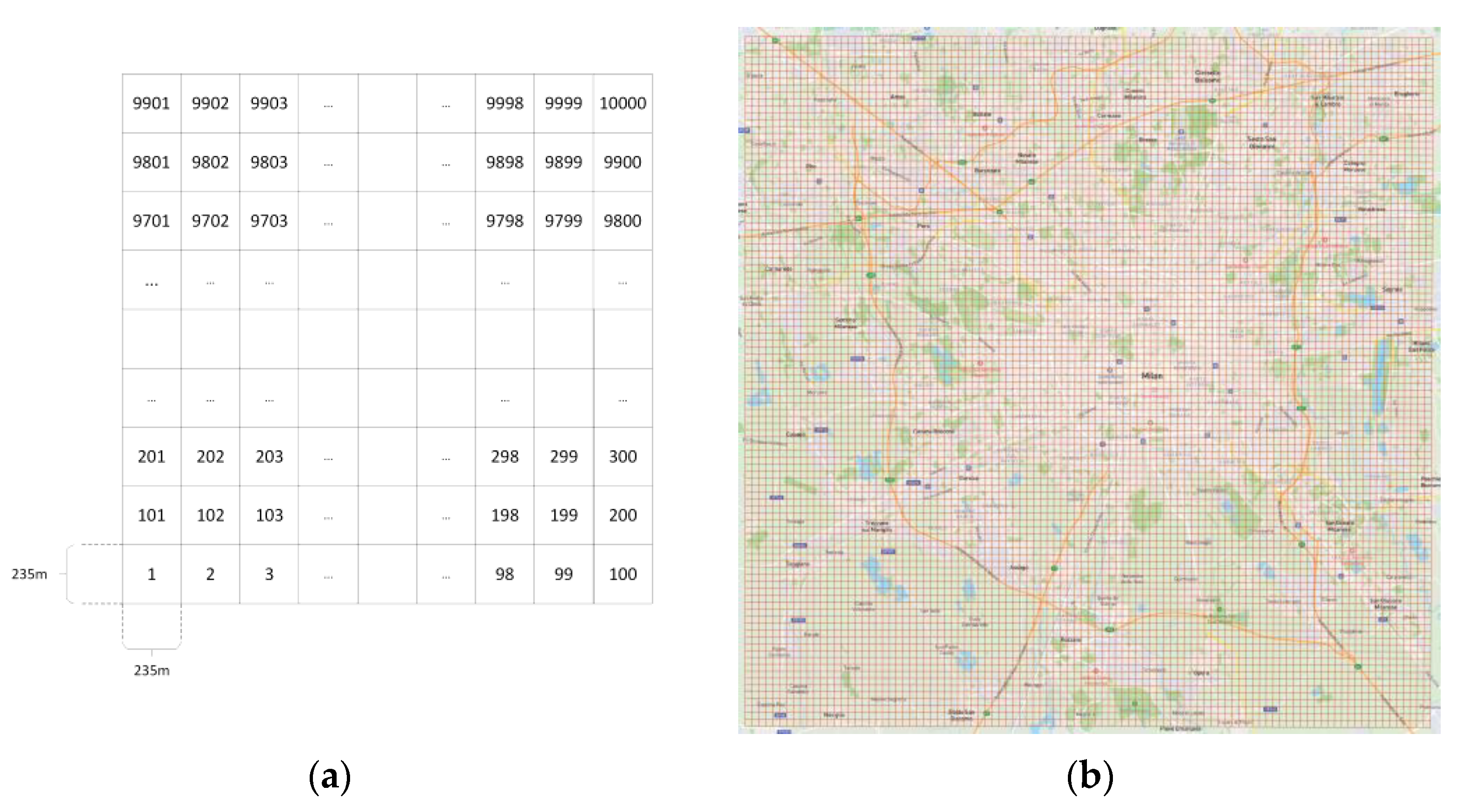
Figure 1. The Basic information of Milan grid division: (a) the grid ID identification and the method of Milan grid division; (b) the specific situation of Milan grid division.
Processes 11 02257 g001
Figure 2. Data pre-processing process.
Processes 11 02257 g002
Figure 3. Distribution of wireless traffic for the 30th cell in temporal distribution.
Processes 11 02257 g003
Figure 4. Distribution of wireless traffic in Spatial distribution.
Processes 11 02257 g004
Figure 5. Quantitative expression of spatial correlation using Pearson’s coefficient.
Processes 11 02257 g005
Figure 6. Graph-structure of cellular network traffic data.
Processes 11 02257 g006
Figure 7. Time series of cellular network traffic data.
Processes 11 02257 g007
Figure 8. The framework of STP-GLN. X C is hourly sequence. X P is daily sequence. X W is weekly sequence. A is adjacency matrix; d a t a is historical time series. Y is the ground truth; Y ^ is the forecasted value.
Processes 11 02257 g008
Figure 9. Prediction results on the SMS dataset of a random selected cell.
Processes 11 02257 g009
Figure 10. Error results on the SMS dataset of a random selected cell.
Processes 11 02257 g010
Figure 11. Prediction results on the Call dataset of a random selected cell.
Processes 11 02257 g011
Figure 12. Error results on the Call dataset of a random selected cell.
Processes 11 02257 g012
Figure 13. Prediction results of the Internet dataset of a random selected cell.
Processes 11 02257 g013
Figure 14. Error results of the Internet dataset of a random selected cell.
Processes 11 02257 g014
Table 1. Dataset information.
ParametersValue
LocationMilan, Italy
Span of time1 November 2013~1 January 2014
Time interval10 min
Type of data{SMS-in, SMS-out, Call-in, Call-out, Internet}
Table 2. Parameters of training model.
ParametersValue
Observation window1056
Forecast window264
Epoch50
Batch size32
Learning rate0.001
Optimization technologyAdam
Loss functionMSE
Training set: test set8:2
Table 3. RMSE, MAE, and R2 of each model on the SMS dataset.
ModelSMS-in (One Cell/All Cells)SMS-out (One Cell/All Cells)
RMSEMAER2RMSEMAER2
HA60.42844.431−0.26625.77219.0400.275
LR15.323/77.85310.845/48.3670.935/0.49213.85/49.8938.434/28.7060.82/0.219
GCN4.888/26.0503.301/14.800.991/0.9755.397/26.7473.705/13.1730.975/0.908
LSTM5.843/37.4154.362/18.4980.989/0.9485.593/32.3473.971/16.1700.985/0.869
STDenseNet [18]6.255/59.9203.768/33.8390.930/0.6407.003/41.3265.812/21.5140.813/0.025
STGCN [25]5.254/46.2974.297/21.1720.92/0.7926.866/35.6595.811/16.5620.906/0.622
STP-GLN2.773/27.3592.038/14.7260.992/0.9732.535/23.51.56/12.3120.984/0.932
Table 4. RMSE, MAE, and R2 of each model on the Call dataset.
ModelCall-in (One Cell/All Cells)Call-out (One Cell/All Cells)
RMSEMAER2RMSEMAER2
HA41.06532.875−0.78650.61340.354−0.816
LR8.355/32.785.682/21.4030.94/0.7807.901/40.255.291/25.1470.953/0.796
GCN1.678/17.5151.184/9.0580.991/0.9772.004/16.9891.499/9.3530.990/0.982
LSTM2.412/17.8541.784/9.8060.991/0.9762.962/20.2582.076/11.1530.988/0.974
STDenseNet [18]3.590/35.8701.999/22.7640.917/0.7193.871/40.8312.212/25.1560.922/0.736
STGCN [25]4.188/22.3982.61/11.4870.951/0.9015.427/25.8373.253/12.7660.962/0.908
STP-GLN1.802/14.3141.216/7.9060.996/0.9851.802/16.2021.708/9.1080.995/0.984
Table 5. RMSE, MAE, and R2 of each model on the Internet dataset.
ModelInternet (One Cell/All Cells)
RMSEMAER2
HA727.021476.142−0.126
LR169.3/514.304127.405/329.3020.964/0.769
GCN113.274/314.83580.15/182.0440.990/0.968
LSTM78.02/290.84154.331/173.8890.994/0.973
STDenseNet [18]186.298/385.376139.712/276.1090.974/0.857
STGCN [25]147.189/267.267108.549/174.3340.974/0.910
STP-GLN27.003/256.44218.82/152.240.995/0.979
Table 6. RMSE, MAE, and R2 of each model on the CIKM21-MPGAT dataset.
ModelCIKM21-MPGAT Dataset
RMSEMAER2
STGCN [25]11.782/15.0884.491/5.5710.522/0.577
STP-GLN3.857/5.2731.28/1.6620.967/0.995
Disclaimer/Publisher’s Note: The statements, opinions and data contained in all publications are solely those of the individual author(s) and contributor(s) and not of MDPI and/or the editor(s). MDPI and/or the editor(s) disclaim responsibility for any injury to people or property resulting from any ideas, methods, instructions or products referred to in the content.