Abstract
Dual-layer pipe dual-gradient drilling technology is an emerging technology for solving the problem of the narrow safety density window in deepwater drilling. The unstable spacer fluid interface in this technology directly affects the dual-gradient pressure system in the annulus, causing changes in the drilling mud performance and affecting the control of bottom hole pressure and rock removal with drilling mud. Therefore, the key to the stable operation of dual-layer pipe dual-gradient drilling technology is to maintain the stability of the spacer fluid interface. Based on this, a seawater-spacer fluid-drilling mud annular flow model was established in this study, with a bottom hole pressure control step of 0.2 MPa, and the spacer fluid height after a single control was used as the evaluation index to study the influence of annular flow velocity, the spacer fluid properties, and the drill string rotation speed on the stability of the spacer fluid interface. The results show that in the determined conditions of the seawater and drilling mud system, the annular fluid flow rate and the physical parameters of the spacer fluid are the main factors affecting the stability of the spacer fluid interface. When the annular fluid flow rate increased within the range of 0.04~0.2 m/s, the liquidity index of the spacer fluid increased between 0.5 and 0.9, the consistency coefficient increased in the range of 0.6 to 1.4 , and the stability of the spacer fluid interface decreased. However, the stability of the spacer fluid interface increased with the increase in its density in the range of 1100~1500 kg/m3. The results obtained in this study can provide a reference for selecting the operating parameters to ensure the stable operation of dual-gradient pressure systems.
1. Introduction
Deepwater oil and gas fields accounted for 67% of the discoveries made and 68% of the reserves developed across the world in the past ten years, and the deepwater area has become an essential field for oil and gas exploration and development [1]. However, deepwater oil and gas resource development involves a narrow safety density window between the formation pore pressure and fracture pressure. Dual-gradient drilling technology is a necessary technical means by which to solve this problem [2,3,4,5,6,7,8].
Currently, three types of dual-gradient drilling technologies are used internationally: riserless drilling technology, subsea pump lifting drilling technology, and dual-density dual-gradient drilling technology [9]. The technology of riserless drilling is mainly used for surface drilling. AGR’s Riserless Mud Recovery (RMR) system is a typical example of this technology. It collects drilling mud and cutting flow back through a suction module installed at the subsea wellhead and transports this fluid to the subsea disc pump through a suction hose, which is then lifted to the surface drilling platform through the mud return line, achieving the recycling of the drilling mud [10,11]. This technology is highly capable of well control in shallow, hazardous areas. It has a low rig payload and space requirements for the drilling rig because it does not use riser pipes or auxiliary equipment. RMR technology has been successfully applied in over 1000 wells globally including the Caspian, North, and other seas [12]. Controlled annular mud level (CAML) technology is an extension of RMR technology and is used after the installation of riser pipes and blowout preventer assemblies [13]. This technology can detect kick and leakage earlier and achieve controlled pressure cementing [14,15]. It has been successfully used in Brazil and the Mediterranean offshore as well as in the North Sea, the Barents Sea, and other seas. Subsea pump lifting drilling technology is represented by the SMD system developed by Conoco and Hydril, the DEEPVISION system developed by Baker Hughes and Transocean Sedco Forex, and the SSPS system developed by Shell. Drilling mud enters the wellbore through the drill pipe and drill bit and returns to the seafloor, where it changes direction and enters the solid phase treatment device to crush large solid particles. After treatment, the mud enters the subsea mud lift pump and is sent to the surface through the mud return line into the mud circulation tank. This technology saves time and costs and can be converted to conventional drilling [16]. The dual-density dual-gradient drilling technique involves the mixing of drilling mud with a low-density medium to dilute it to a low-density fluid, which is then injected into the bottom of the riser to reduce the density of the drilling mud inside the riser and create two different pressure gradients in the riser annulus and wellbore annulus [17]. Transocean’s Continuous Annular Pressure Management system (CAPM), the LSU and BR’s gas lift dual-gradient drilling system, and the MTI’s hollow sphere dual-gradient drilling system are typical of this technology [18,19,20,21].
Dual-layer pipe dual-gradient drilling technology is new in this field. This technology can be converted to conventional drilling technology, and the mud lift pump used is driven by seawater, so the system has high reliability [22,23]. As shown in Figure 1, in this technology, drilling mud enters the bottom of the wellbore from the annulus of the dual-layer pipe and is lifted to the water surface through the inner pipe of the dual-layer pipe by the bottom mud lift pump. Therefore, this technology has strong rock-carrying and wellbore-cleaning capabilities. The spacer fluid separates the seawater in the annulus of the riser pipe and drilling mud in the annulus of the wellbore to realize the dual-gradient pressure system. The flow rate control unit on the water surface regulates the flow rate of the drilling mud in the inflow pipeline and the opening of the throttle valve in the return fluid pipeline, thereby controlling the lift and displacement of the bottom mud lift pump to realize the upward and downward movement of the spacer fluid in order to ensure that the bottom hole pressure is always within the safe density window [24,25]. Therefore, the stable operation of the dual-gradient pressure system, consisting of seawater, spacer fluid, and drilling mud, is the key to controlling bottom hole pressure. The spacer fluid is an essential component of this dual-gradient pressure system, and a stable spacer fluid interface is the primary prerequisite for the stable operation of the pressure system. However, dual-layer pipe dual-gradient drilling technology is still in the development stage, and there is a lack of research on the stability of the spacer fluid interface.
It is found that the study of cementing displacement interface has reference value for exploring the stability of the spacer fluid interface in dual-layer pipe dual-gradient drilling. However, most of the existing research on cementing displacement has only been carried out using the displacement analysis of the two-phase fluid, drilling mud/spacer fluid, spacer fluid/cement slurry, drilling mud/cement slurry [26,27,28,29,30,31,32], which is different from the three-phase movement of annular seawater, spacer fluid, and drilling mud in dual-layer pipe dual-gradient drilling. In addition, the cementing displacement annulus does not need to consider the influence of the drill string, but the flow of the spacer fluid in the annulus in dual-layer pipe dual-gradient drilling will be affected by the drill string disturbance, which puts higher requirements on the stability of the spacer fluid interface. Therefore, it is necessary to combine the technical background and characteristics of dual-layer pipe dual-gradient drilling to analyze the flow of three-phase fluids in the annulus and explore the influence of various factors on the stability of the spacer fluid interface.
Based on the above situation, a seawater-spacer fluid-drilling mud annular flow simulation model was established in this study, with a bottom hole pressure control step of 0.2 MPa, and the spacer fluid height after a single control was used as the evaluation index to study the influence of annular flow velocity, the spacer fluid properties, and drill string rotation speed on the stability of the spacer fluid interface. The results show that annular flow velocity and the spacer fluid properties significantly affect the interface’s stability, but the rotation speed of the drill string has a negligible effect. This research can provide a reference for the development of dual-layer pipe dual-gradient drilling technology.
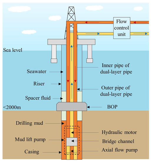

Figure 1.
The dual-layer pipe dual-gradient drilling system [33].
Figure 1.
The dual-layer pipe dual-gradient drilling system [33].
2. Simulation Model Specification
Model setting is the foundation for conducting simulations, and it consists of five parts: establishing the physical model, basic governing equations, materials, and boundary conditions, and formulating evaluation criteria for the stability of the spacer fluid interfaces and model validation.
2.1. Physical Simulation Model
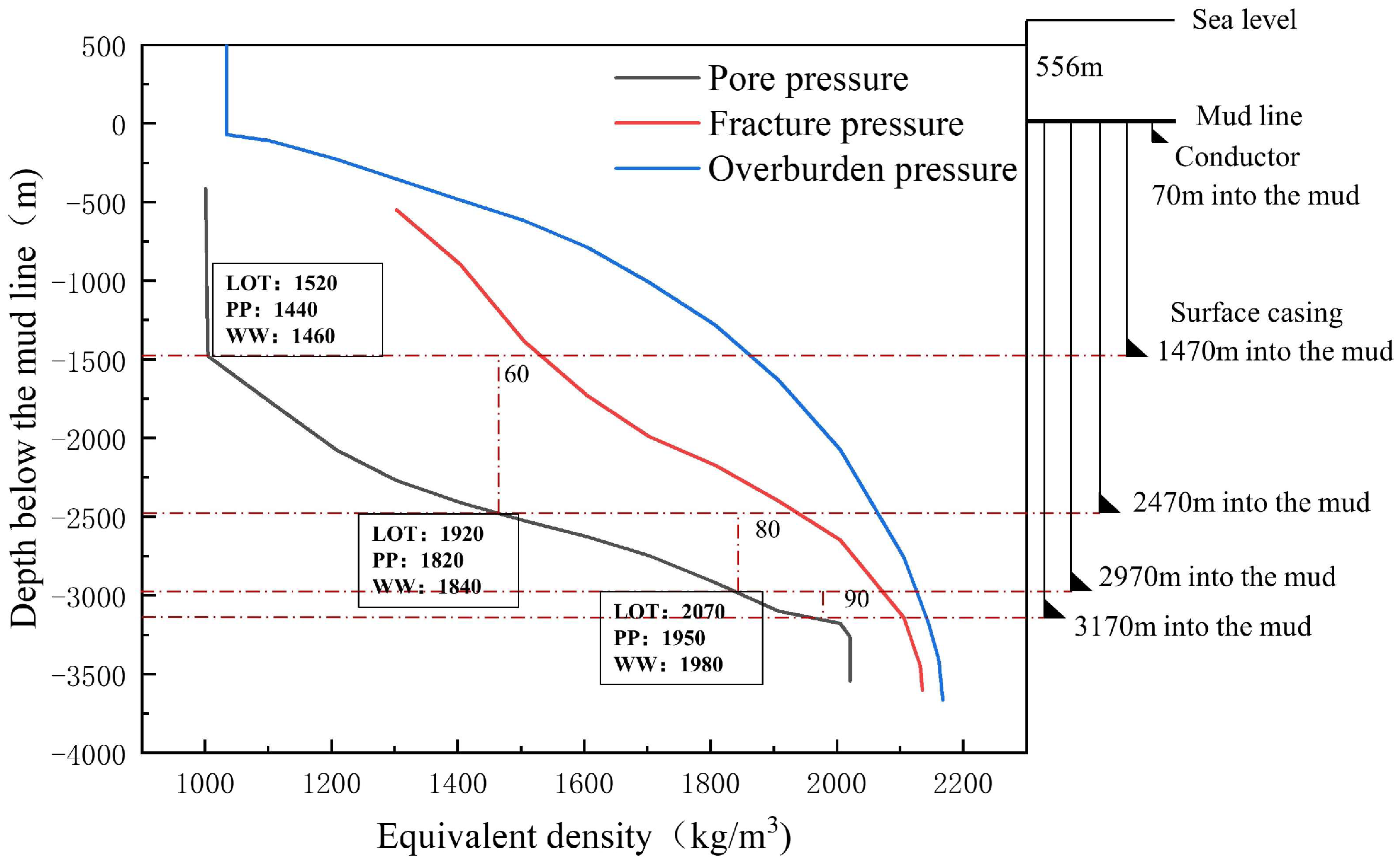
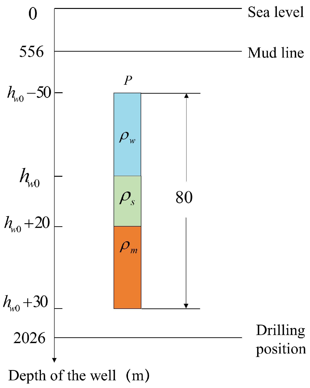
In conventional drilling, the drilling mud system is designed based on the pressure prediction profile from logging to maintain the bottom hole pressure within the safe window for a certain well section. However, the large pressure difference between the bottom hole and formation pressure can affect the rate of penetration (ROP) [34,35]. Therefore, to minimize the bottom hole pressure difference and improve the drilling efficiency, this paper adopted the dual-layer dual-gradient drilling method for a LS well, as shown in Figure 2, by continuously adjusting the bottom hole pressure to be within the safe density window and ensure a low bottom hole pressure difference.
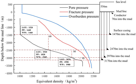
Figure 2.
Partial pressure profile and well structure of a LS well.
According to Figure 2, the surface drilling is completed below the mud line at 1470 m, 2026 m below sea level. Starting from this level, dual-layer pipe dual-gradient drilling is used. The safe density window at this location is (1030, 1520). Considering the drilling mud density additional value of 70 kg/m3 and the equivalent density of the target bottom hole pressure of 1100 kg/m3, the spacer fluid position corresponding to this equivalent density is the optimal position. Assuming that the height of the spacer fluid in the dual-gradient pressure system is 20 m, establishing the seawater-spacer fluid-drilling mud pressure system to start drilling after the spacer fluid is in the optimal position. As shown in Figure 3, when the pressure difference between the actual bottom hole pressure and the target bottom hole pressure reached 0.2 MPa, the position of the spacer fluid was adjusted once to ensure that the bottom hole pressure was equal to the target bottom hole pressure.
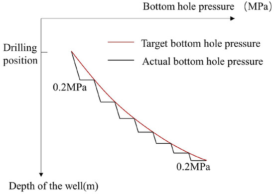
Figure 3.
The variation in bottom hole pressure with well depth when the regulation step is 0.2 MPa.
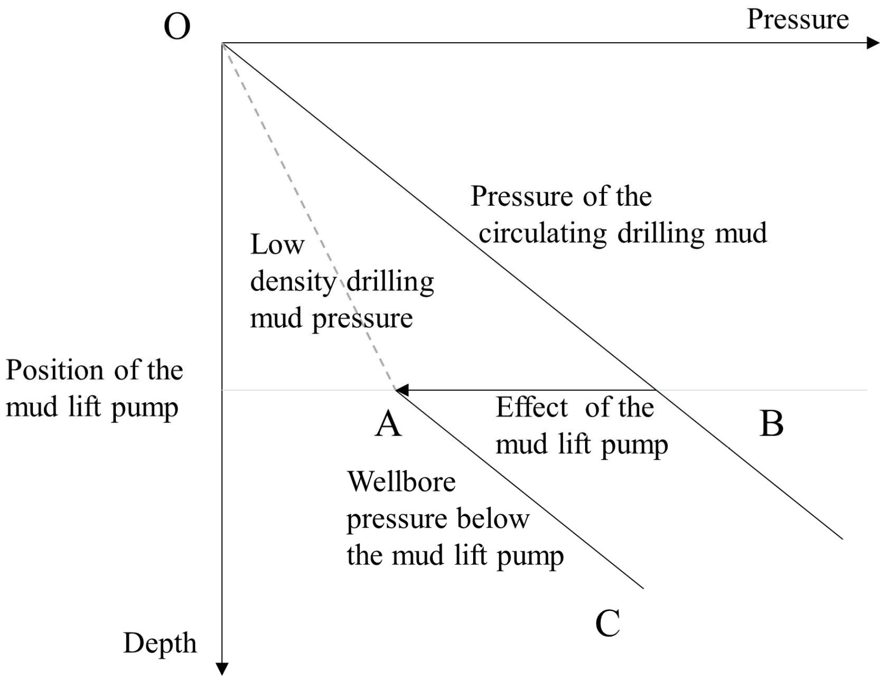
As shown in Figure 4, the bottom hole pressure expression of dual-layer pipe dual-gradient drilling with no fluid flow in the annulus is [33]
where the unit of is MPa; are the density of the seawater, spacer, and drilling mud, respectively, kg/cm3; are the height of the seawater, spacer fluid, and drilling mud, respectively, m; is the equivalent density, kg/cm3; is the equivalent well depth, m. The expression for is
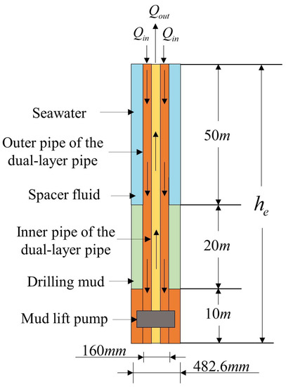
Figure 4.
The formation and control principles of the bottom hole pressure in a dual-layer pipe dual-gradient drilling system.
From Equations (1) and (2), the expression for seawater height is
where can indirectly indicate the spacer fluid position.
The actual working conditions are complex and changeable, and five assumptions were adopted in this paper:
- (1)
- All fluids are incompressible;
- (2)
- Both the spacer fluid and drilling mud are pseudoplastic fluids;
- (3)
- The wellbore is uniform, and variations in wellbore diameter and the effects of the dual-layer pipe joints are ignored;
- (4)
- The annulus is rigid with smooth walls;
- (5)
- Due to the small control step of 0.2 MPa for the bottom hole pressure and the low drilling speed during actual drilling, the equivalent well depth change caused by drilling during the process of reaching the pressure difference and during the regulation of bottom hole pressure can be ignored.
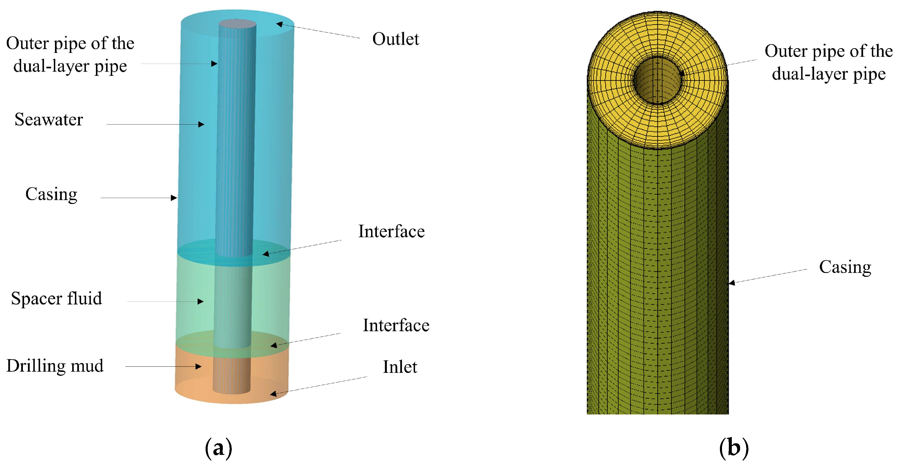
The geometric parameters used for the simulation are shown in Table 1. A three-dimensional model was established to simulate the annular fluid flow between the outer pipe of the dual-layer pipe and the casing. The ICEM divides the hexahedral mesh, and the grid is refined in the near-wall area, as shown in Figure 5.

Table 1.
Geometric parameters of the simulation model.
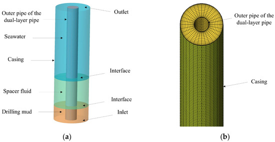
Figure 5.
Model diagram: (a) geometric model; (b) grid model.
2.2. Basic Governing Equation
This study utilized FLUENT as its numerical software [31], employing the k-epsilon model and species transport model. The relevant governing equations are as follows:
- (1)
- Continuity and Momentum Equations
The equation for the conservation of mass, or continuity equation, can be written as follows:
where the source is the mass added to the continuous phase from the dispersed second phase and any user-defined sources.
Momentum conservation equations:
where is the static pressure; and are the gravitational body force and external body forces, respectively; also contains other model-dependent source terms such as porous-media and user-defined sources; is the stress tensor, where is the molecular viscosity, is the unit tensor, and the second term on the right-hand side is the effect of volume dilation.
The change in heat during the flow of incompressible fluids is very small, and the energy equation can be neglected.
- (2)
- Species transport equations
- (3)
- Transport equations for the standard model
The turbulence kinetic energy, , and its rate of dissipation, , are obtained from the following transport equations:
where represents the generation of turbulence kinetic energy due to the mean velocity gradients; is the generation of turbulence kinetic energy due to buoyancy; represents the contribution of the fluctuating dilatation in compressible turbulence to the overall dissipation rate; the turbulent viscosity ; , and are the recommended values of 1.44, 1.92, 0.09, 1.0, and 1.3, respectively; and are user-defined source terms.
2.3. Materials and Boundary Conditions
The physical parameters of the materials used are shown in Table 2.
Table 2.
Physical parameters of the materials.
In this paper, the boundary of two different fluids was set as the interface. The inner wall of the annular space is also the outer pipe of the dual-layer pipe, which was set as the rotating wall. The boundary conditions of the velocity inlet and pressure outlet were adopted, and the specific values are as follows:
- (1)
- Inlet boundary:
As shown in Figure 4, the bottom hole pressure control principle of dual-layer pipe dual-gradient drilling is as follows. When it is necessary for the bottom hole equivalent density to decrease, one adjusts the mud lift pump to cause the drilling mud in the casing annulus to decrease, the position of the spacer fluid to drop, and the bottom hole pressure to decrease. Conversely, when the bottom hole equivalent density is required to increase, the position of the spacer fluid should be raised. Therefore, the magnitude of the annular fluid flow rate is determined by the drilling mud flux difference between the inflow and outflow of the dual-layer pipe. If one needs to reach the target bottom hole pressure as soon as possible, it should be as large as possible, assuming that it is 35 L/s (the design index of the mud lift pump is 35 L/s), that is, all 35 L/s of the inflow is used for bottom hole pressure control. Currently, the maximum movement rate of the annular fluid is 0.21 m/s. Therefore, the actual movement rate of the annular fluid during control should be less than 0.21 m/s; the inlet flow rate should be less than 0.21 m/s.
- (2)
- Outlet boundary:
The positional relationship of the model throughout the whole well at the beginning of regulation is shown in Figure 6.

Figure 6.
Positional relationship of the model throughout the whole well.
- (1)
- Initially, the expression for the actual wellbore pressure at the top of the model is
- (2)
- During regulation, the height of the seawater in the annulus decreases, but the top of the model is always the seawater until the end of regulation; then, the expression for the actual wellbore pressure at this location is
If Q and are the maxima, the calculated circulating pressure depletion of the seawater beyond the top of the model is no greater than 0.08 MPa; thus, the value can be ignored. Therefore, during the regulation process, the actual wellbore pressure at the top of the model is consistent with the wellbore pressure at this position in the initial state. Specifically,
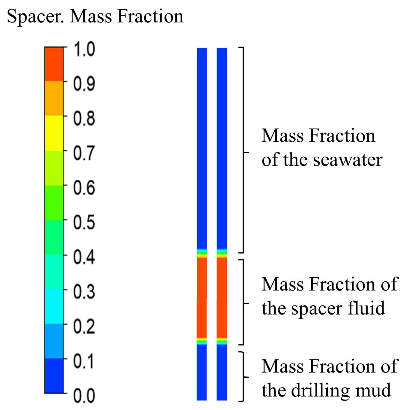
As shown in Figure 7, there are two stable interfaces between the seawater, spacer fluid, and drilling mud in the transient model under the initial conditions.
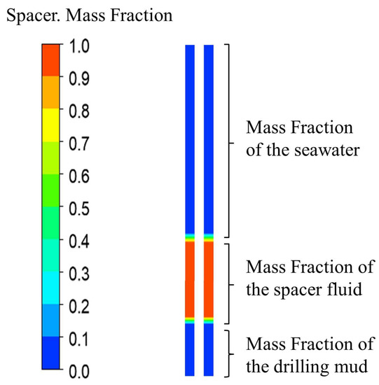
Figure 7.
Cloud atlas of the spacer fluid mass fraction profile under the initial conditions.
2.4. Evaluation Criteria
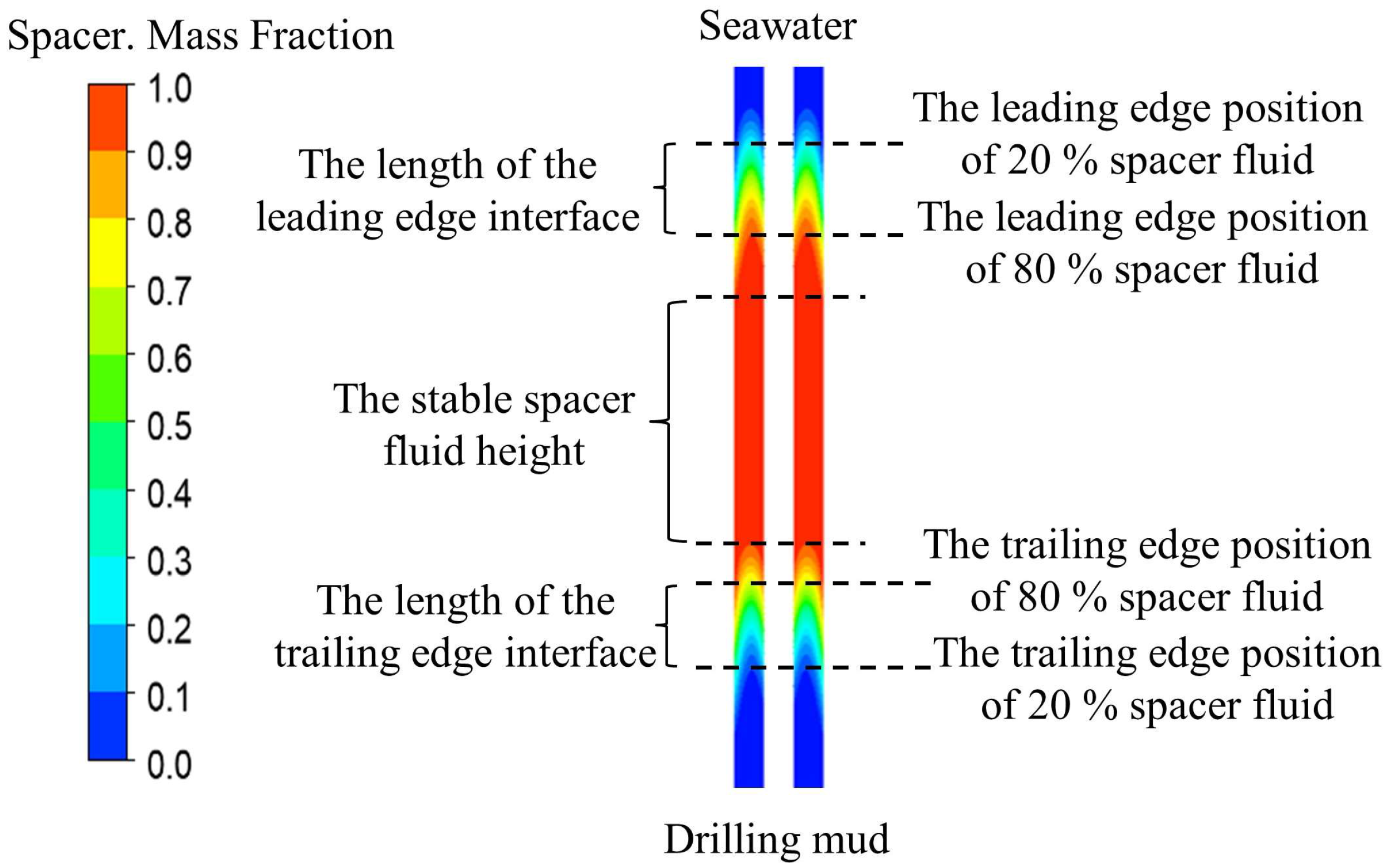
The spacer fluid is regarded as the interface between the seawater and drilling mud, and the stability of the spacer fluid interface refers to its ability to separate the seawater from the drilling mud. As shown in Figure 8, this paper evaluated the stability of the spacer fluid interface with the spacer fluid height in the annulus after a single adjustment of the bottom hole pressure as an index. In addition, the length and shape of the spacer fluid’s leading and trailing edge interfaces were used as auxiliary references.
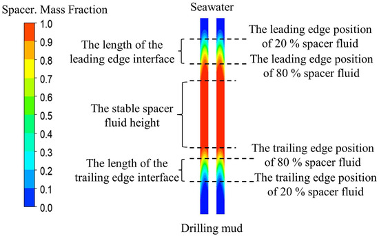
Figure 8.
Setting of the stability evaluation indicators for the spacer fluid interface. The position of the 20% spacer fluid indicates the location where the mass fraction of the spacer fluid is 20% on the cross-section.
- (1)
- The length of the leading edge interface, which is the interface length between the seawater and spacer fluid, evaluates the degree of mixing between the spacer fluid and seawater.
- (2)
- The length of the trailing edge interface, which is the interface length between the drilling mud and spacer fluid, evaluates the degree of mixing between the spacer fluid and drilling mud.
- (3)
- The spacer fluid height, which is the height of the spacer fluid with 100% mass fraction in the annulus, is used to assess the stability of the spacer fluid interface, and the higher this height is, the more stable the spacer fluid interface.
The length of the leading and trailing edge interfaces and the spacer fluid height can be obtained by writing a custom function to record the mass fraction of the spacer fluid at each grid height. Consider a response time of 20 s, which refers to the time consumed from detecting the wellbore pressure regulation completion to when the signal of stopping regulation transmits to the annulus. Assuming that the annulus fluid is regulated at the maximum flow rate, to ensure the stability of the spacer interface, the spacer height must be greater than 4.2 m at the end of regulation. Taking 4.2 m as the standard, if the spacer fluid height is within the range of 3.36 m to 4.2 m, which is within 80%, the spacer fluid interface is considered relatively stable; if the height is less than 3.36 m, the spacer fluid interface is unstable.
2.5. Model Validation
- (1)
- Grid independence verification
According to the principle of custom function writing in this article, the calculation of interface length is closely related to the setting of the grid scale in the flow direction. Therefore, it is necessary to study the influence of the grid scale in the flow direction. As shown in Table 3, when the flow direction grid step was reduced to 0.1 m, the error was within 5%, and the error change was minimal when the grid scale was further reduced. Therefore, the flow direction grid step was determined to be 0.1 m. The number of grids used in the simulation model is 512,000.
Table 3.
Grid scheme and results of the flow direction.
- (2)
- Model Validation
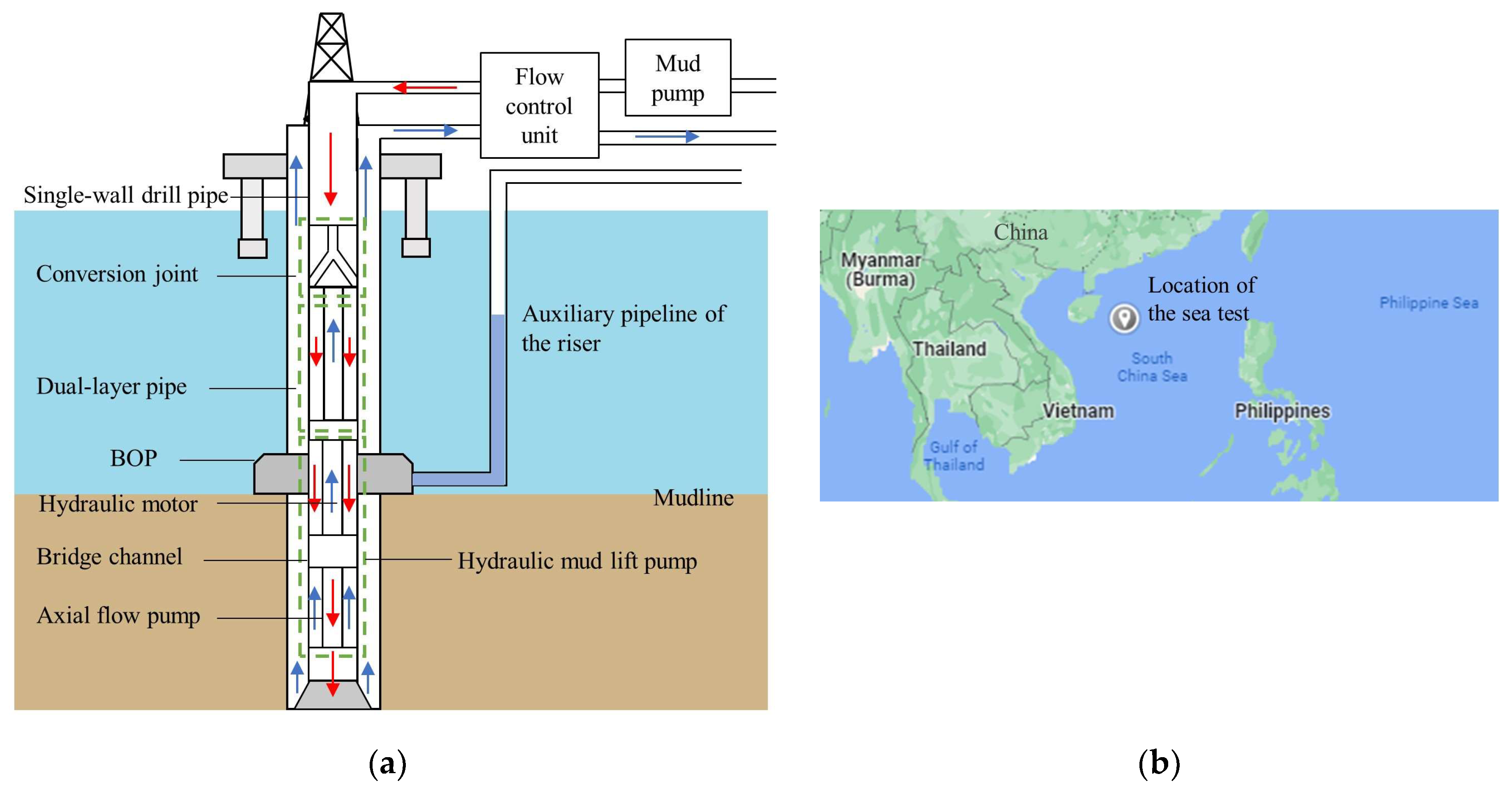
In order to verify the feasibility of the principle of the dual-layer pipe dual-gradient drilling technology, we designed an offshore test system, mainly consisting of a drilling platform, single-wall drill pipe, conversion joint, dual-layer pipe, hydraulic mud lift pump, etc. The offshore test was conducted in a certain sea area with a depth of 1300 m in the South China Sea. Figure 9 shows the location and schematic diagram of the offshore test of the dual-layer pipe dual-gradient drilling technology, and the flow direction of the circulating drilling mud is shown as the arrows in the figure. Since only one dual-layer pipe is used in the offshore test, the riser annulus achieves the effect of drilling mud backflow in the dual-layer pipe string. We closed the annular blowout preventer to separate the outlet and inlet of the hydraulic mud lift pump so that the mud lift pump could work to realize the dual-gradient drilling effect, as shown in Figure 10. In addition, the riser’s auxiliary pipeline simulates the annulus’s impact between the dual-layer pipe and the riser, which can reflect the bottom hole pressure and verify the control mechanism of the dual-layer pipe dual-gradient drilling technology.
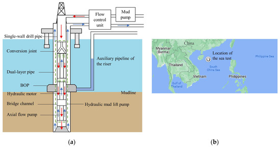
Figure 9.
Offshore test of the dual-layer pipe dual-gradient drilling system: (a) offshore test schematic diagram; (b) location of the offshore test.

Figure 10.
Application principle of the mud lift pump in dual-gradient drilling.
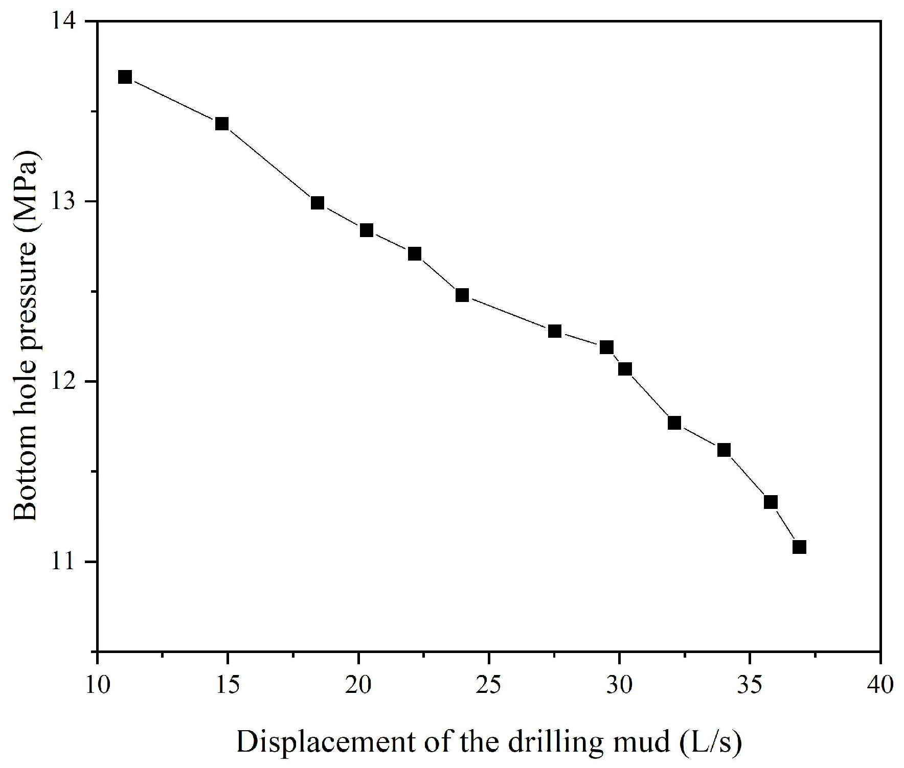
The experiment changed the displacement of the drilling mud to alter the head of the mud lift pump, thus regulating the bottom hole pressure. The experimental results are shown in Figure 11. It can be seen that the mud lift pump and experimental system we designed could reduce the bottom hole pressure by 2.67 MPa. This can be converted so that the equivalent density control range of the bottom hole at a 1000 m water depth is 271 kg/m3, which verifies the correctness and feasibility of the principle of dual-layer dual-gradient drilling technology.
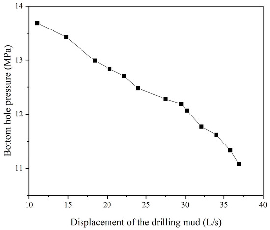
Figure 11.
Relationship between drilling mud displacement and bottom hole pressure in the offshore test.
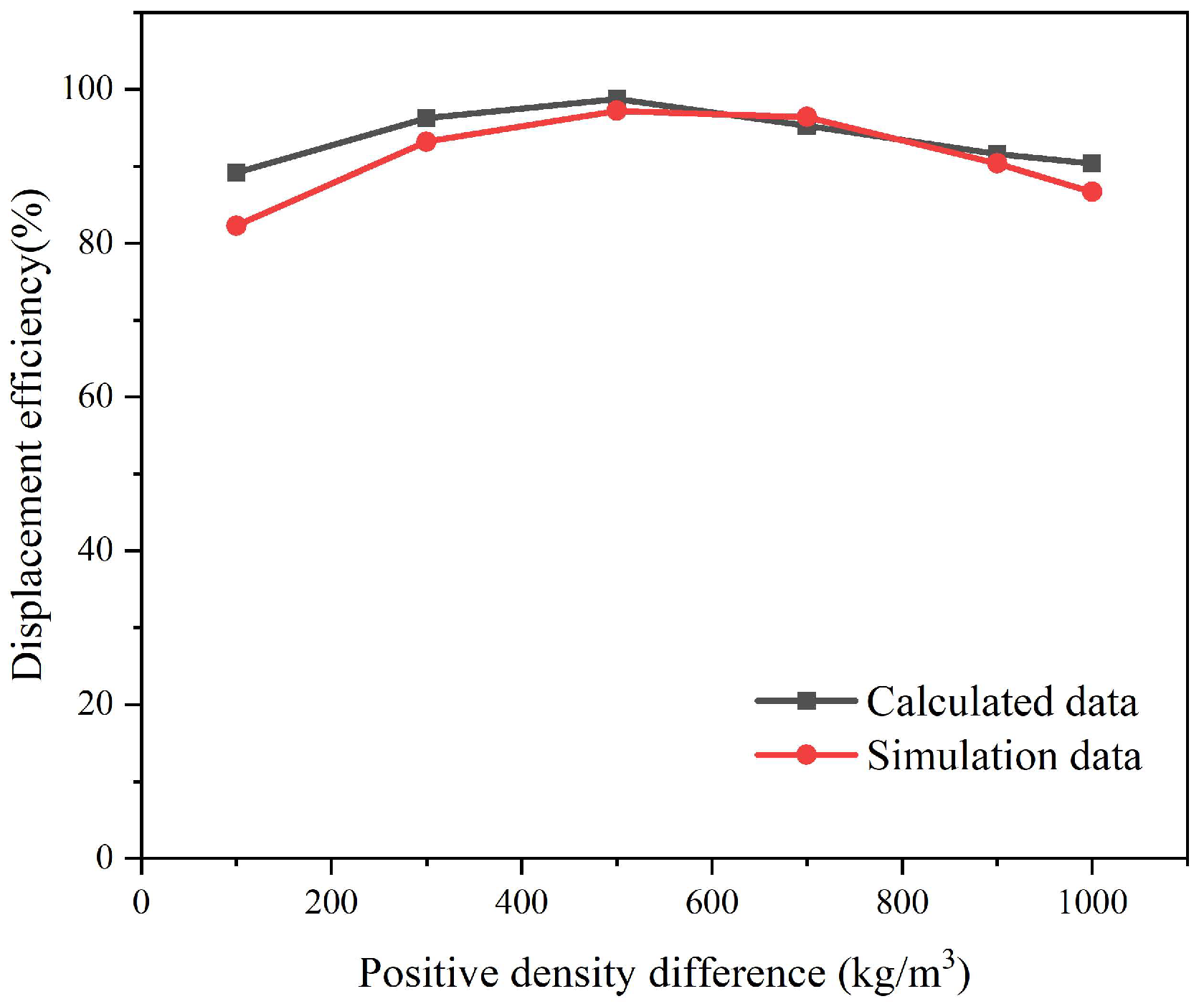
Based on the feasibility of the principle of the dual-layer pipe dual-gradient drilling technology, we verified the correctness of the established model. According to the literature, specifically [31] and [32], it can be seen that the flow characteristics of multiphase fluids in the annulus can be described by two parameters: the interface length and displacement efficiency. In this study, the displacement efficiency was indirectly used to verify the model’s accuracy. We extracted the displacement efficiency calculated with different density differences when the inclination angle of the uniform borehole wall is 0, as shown in Table 4 of Ref. [36], and compared it with the data obtained using the model simulation under the same working conditions explored in this paper. The result, as shown in Figure 12, indicates that the deviation of the simulation model used in this paper was less than 10%, which falls within a reasonable range.
Table 4.
The correspondence between the flow difference, flow velocity, and regulation time.
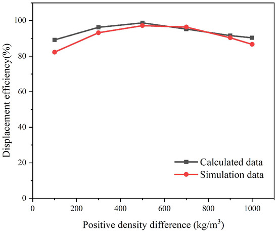
Figure 12.
Comparison of the simulation data and calculated data.
3. Results and Discussion
There are several factors that affect the stability of the spacer fluid interface in dual-layer pipe dual-gradient drilling including the annular fluid flow velocity, spacer fluid density, spacer fluid liquidity index and consistency coefficient, and drill string rotation speed [30,31,37,38].
3.1. The Effects of Annular Fluid Flow Velocity on the Stability of the Spacer Fluid Interface
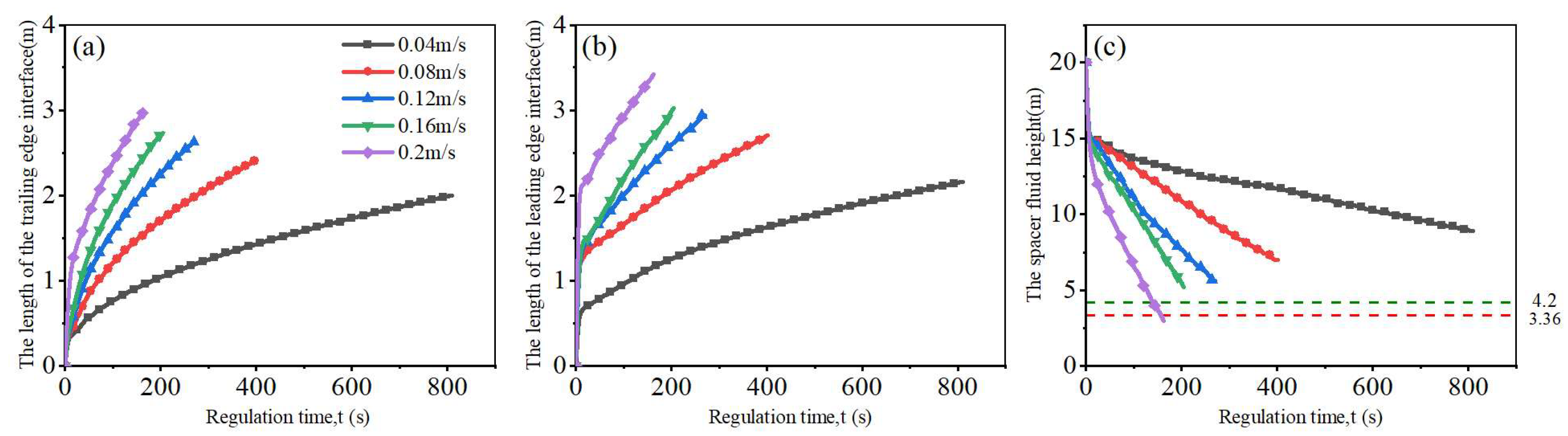
Considering that the movement rate of the annular fluid should be less than 0.21 m/s during bottom hole pressure regulation, the flow differences between the inlet and outlet of 6.5 L/s, 13.0 L/s, 19.5 L/s, 26.0 L/s, and 32.5 L/s were used to study the influence of flow velocity on the stability of the spacer fluid interface. Since the regulation step and the height of the regulated spacer fluid movement are determined, and the time required for regulation is different for different flow rates, the smaller the flow rate, the longer the control time. The corresponding relationships between the flow rate and the required control time at different flow rates are shown in Table 4, and the simulation results are shown in Figure 13.
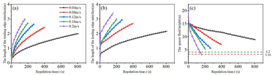
Figure 13.
Effect of flow velocity on the distribution characteristics of the spacer fluid interface: (a) effect of flow velocity on the length of the trailing edge interface; (b) effect of flow velocity on the length of the leading edge interface; (c) effect of flow velocity on the spacer fluid height.
As shown in Figure 13, the length of the leading and trailing edge interfaces increased with the regulation time. As the flow rate increased, the length of the leading and trailing edges interface increased; even though the spacer fluid flow rate of 0.04 m/s required the longest regulation time, the length of the leading and trailing edge interfaces was still the smallest at the end of the regulation. With the increase in the flow rate, the spacer fluid height decreased, and the interface stability decreased. The spacer fluid interface was stable when the flow rate was in the range of 0.04~0.16 m/s. However, when the flow rate increased to 0.2 m/s, the spacer fluid height decreased to just 3 m at the end of regulation, and the spacer fluid interface became unstable.
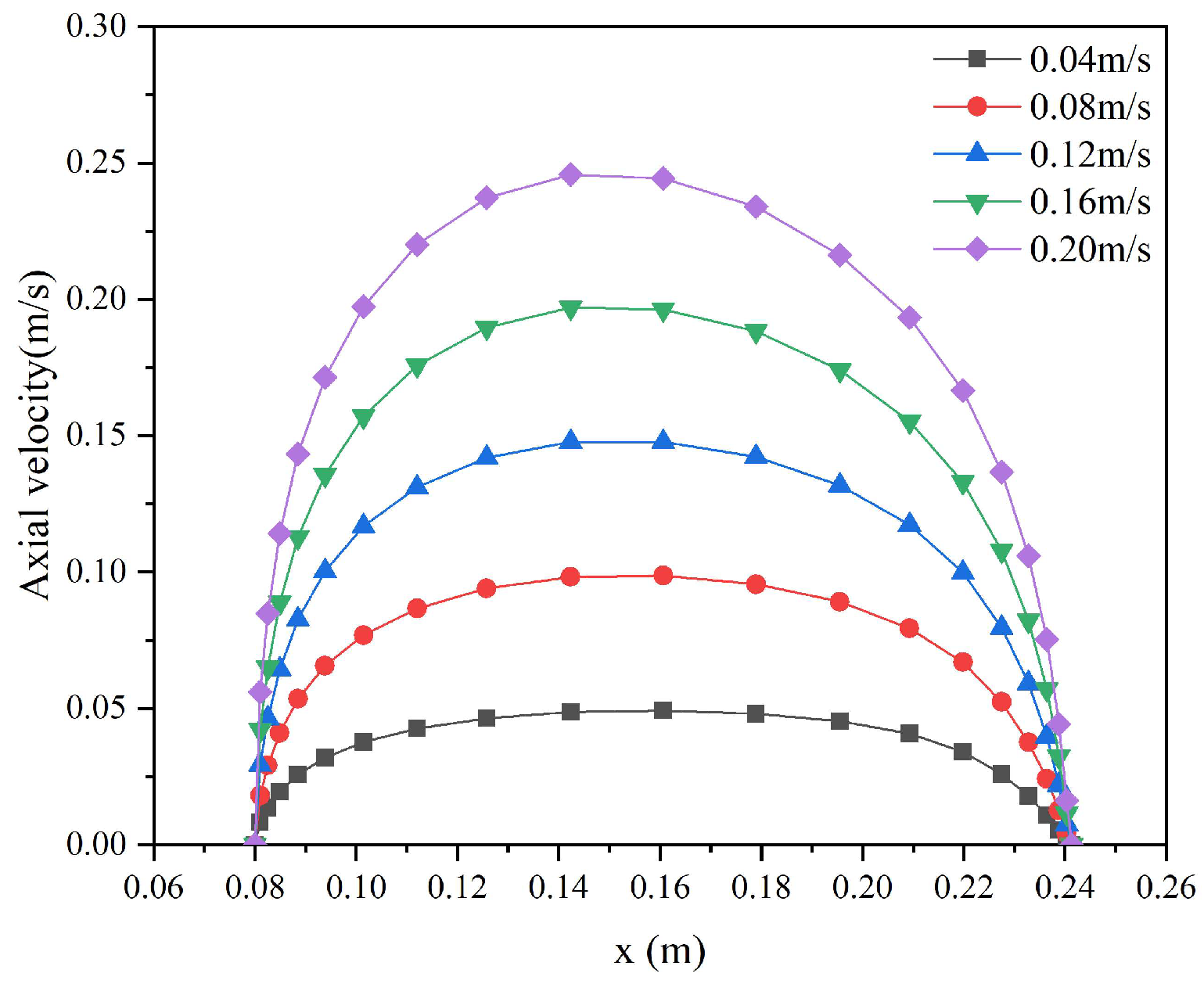
We analyzed the reasons for this phenomenon. As shown in Figure 14, the larger the flow velocity, the larger the velocity gradient between adjacent flow layers, and the unevenness of the axial velocity distribution increases, which leads to an increase in the interface length and a decrease in the height of the spacer fluid. Yang Jiawei also obtained the same rule when studying the influence of displacement velocity on cementing displacement efficiency [39].
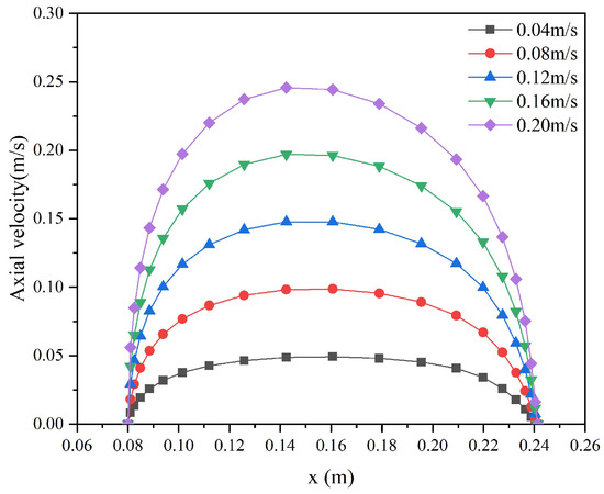
Figure 14.
Axial velocity distribution of different annular flow rates.
3.2. The Effects of Spacer Fluid’s Density on Interface Stability
Based on the design requirements of the spacer fluid, which require that its density is between that of the seawater and drilling mud, we adopted the spacer fluid densities of 1100, 1200, 1300, 1400, and 1500 kg/m3 for the simulation. However, the spacer fluid density affects the height of the seawater in the initial state, thereby affecting the positional relationship of the model throughout the whole well and the pressure boundary conditions at the outlet end. The height of the seawater at different spacer fluid densities and the pressure boundary conditions at the top of the model are shown in Table 5, and the simulation results are presented in Figure 15.
Table 5.
The correspondence between the density of the spacer fluid and the pressure boundary condition, P.
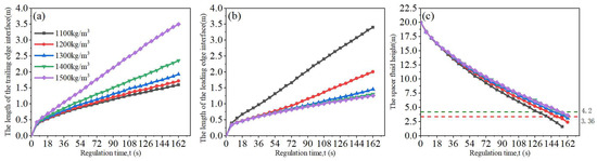
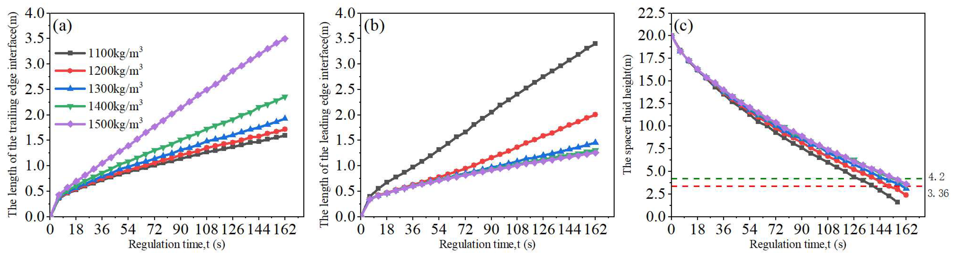
Figure 15.
Effect of the spacer fluid’s density on its interfacial distribution characteristics: (a) effect of spacer fluid’s density on the length of the trailing edge interface; (b) effect of spacer fluid’s density on the length of the leading edge interface; (c) effect of spacer fluid’s density on its height.
Figure 15a shows that the larger the spacer fluid density, the longer the length of the trailing edge interface. With the increase in the spacer fluid density, the trailing edge interface length becomes more sensitive to the change in the spacer fluid density. Significantly, when the density increased from 1400 kg/m3 to 1500 kg/m3, the trailing edge interface length increased further. From Figure 15b, it can be seen that the greater the density of the spacer fluid, the smaller the length of the leading edge interface. When the density of the spacer fluid was between 1300 kg/m3 and 1500 kg/m3, the length of the leading edge interface increased slightly. However, when the density of the spacer fluid was less than 1300 kg/m3, the length of the leading edge interface was susceptible to changes in density. It can be seen from Figure 15c that the greater the density of the spacer fluid, the higher the spacer fluid height and the higher the interface stability. When the density of the spacer fluid was between 1100 kg/m3 and 1300 kg/m3, the interface was unstable. There was no longer a spacer fluid height at the end of regulation when the density was 1100 kg/m3, and the seawater and drilling mud were mixed. Increasing the density of the spacer fluid to 1400~1500 kg/m3 rendered the interface relatively stable.
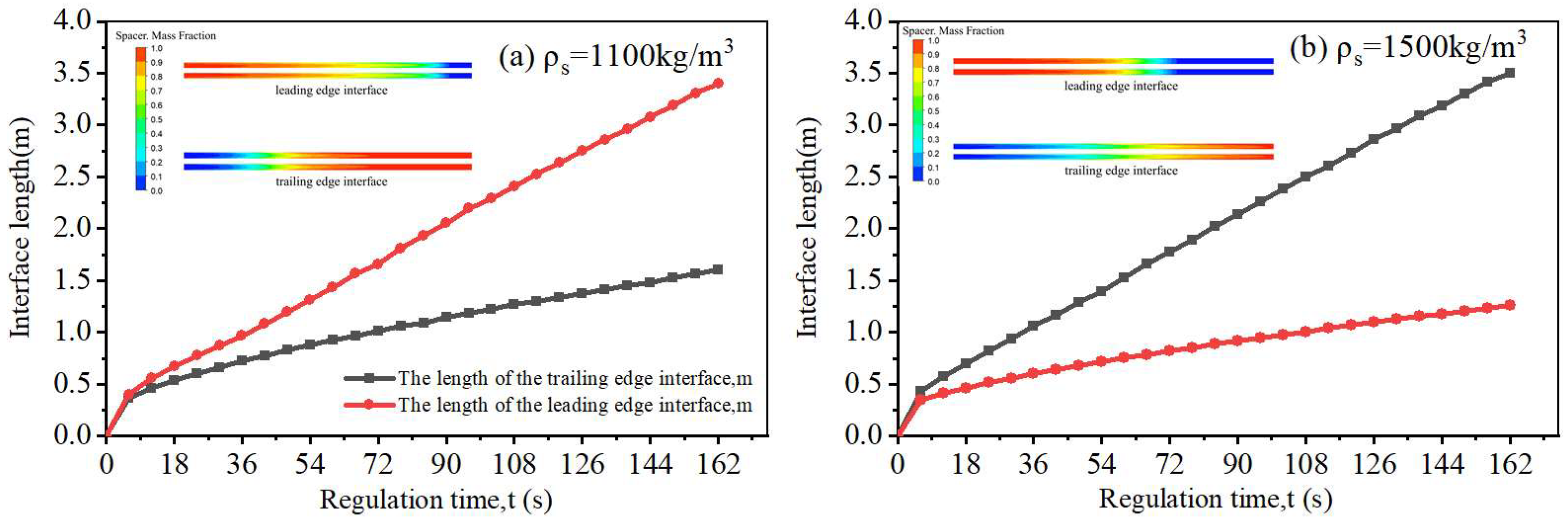
There are differences in the leading and trailing edge interfaces when regulating the bottom hole pressure of the spacer fluid with different densities, mainly due to the differences in the buoyancy effects caused by distinct density differences [36]. As the buoyancy effect generated by a positive density difference can drive the fluid, the more significant the density difference, the more pronounced the buoyancy effect, resulting in a shorter interface length. Figure 16 shows the distribution characteristics of the leading and trailing edge interfaces when the density of the spacer fluid was 1100 kg/m3 and 1500 kg/m3. When the density of the spacer fluid was 1100 kg/m3, its density difference from the drilling mud was 560 kg/m3, while the density difference from the seawater was only 70 kg/m3. The buoyancy effect between the drilling mud and the spacer fluid was more significant, resulting in a shorter length of the rear edge interface. When the density of the spacer fluid was 1500 kg/m3, its density difference from the seawater was 470 kg/m3, while the density difference from the drilling mud was only 160 kg/m3. The buoyancy effect between the seawater and the spacer fluid was more prominent, resulting in a leading edge interface length that was significantly shorter than the trailing edge interface length.
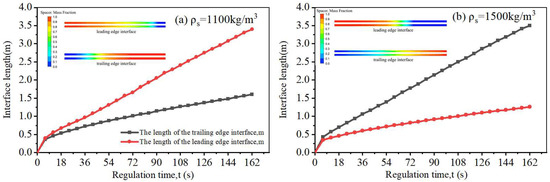
Figure 16.
The shape and length of the leading and trailing edge interfaces at different spacer fluid densities. The cloud diagram shows the interface shape produced by spacer fluids with different densities at the end of regulation: (a) the density of the spacer fluid was 1100 kg/m3; (b) the density of the spacer fluid was 1500 kg/m3.
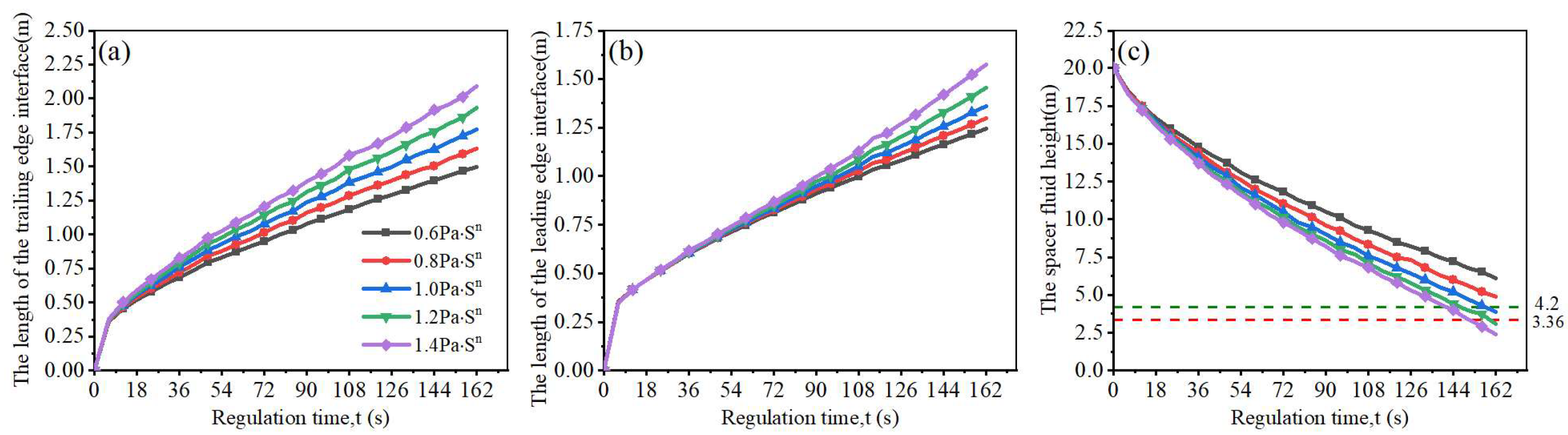
3.3. The Effects of the Spacer Fluid’s Rheological Parameters on Its Interface Stability
- (1)
- Liquidity index of the spacer fluid
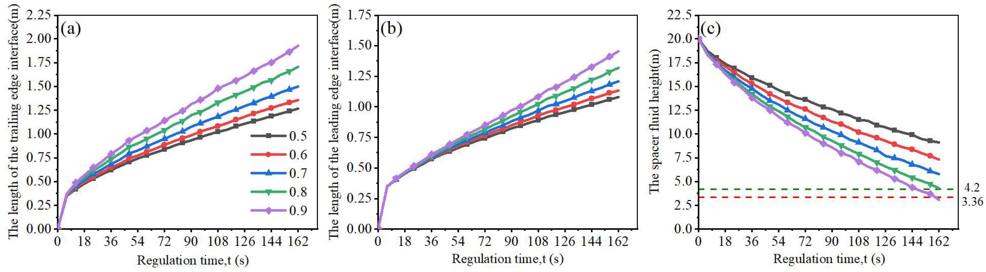
This section discusses the influences of different liquidity indices of the spacer fluid on the stability of the spacer fluid interface when regulating bottom hole pressure. Five spacer fluid liquidity indices were selected for the simulation study, which were 0.5, 0.6, 0.7, 0.8, and 0.9. The simulation results are shown in Figure 17. It can be seen that the greater the liquidity index of the spacer fluid, the longer its leading and trailing edge interfaces become, and the height of the spacer fluid decreases, leading to a decrease in the stability of the interface. When the liquidity index was within the range of 0.5 to 0.8, the interface of the spacer fluid was stable. When the liquidity index was increased to 0.9, the height of the spacer fluid was 3.1 m at the end of regulation, and the interface was unstable. This phenomenon arises because the liquidity index characterizes the degree of fluid deviation from Newtonian fluid. In a pseudoplastic fluid, the smaller the liquidity index, the stronger the shear thinning effect, the flatter the flow velocity profile, the smaller the produced axial velocity difference, and the shorter the interface length, leading to a more stable interface. This is consistent with the results obtained by Wang Binqiao in studying the influence of displaced fluid flow index on the interface length in cementing [32].
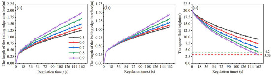
Figure 17.
Effect of the liquidity index of the spacer fluid on its interfacial distribution characteristics: (a) effect of spacer fluid’s liquidity index on the length of the trailing edge interface; (b) effect of spacer fluid’s liquidity index on the length of the leading edge interface; (c) effect of spacer fluid’s liquidity index on its height.
- (2)
- Consistency coefficient of the spacer fluid
The consistency coefficient of the spacer fluid has an impact on its interface. Five spacer fluid consistency coefficients were selected for the simulation study, which were 0.6, 0.8, 1.0, 1.2, and 1.4 . The results are shown in Figure 18. It can be seen that the larger the consistency coefficient of the spacer fluid, the larger the length of the leading and trailing edge interfaces and the lower the height of the spacer fluid, leading to lower interface stability. This pattern is consistent with the research findings of Wang Binqiao [32]. When the consistency coefficient was in the range of 0.6~0.8 , the spacer fluid interface was stable; when the value was increased to 1.0 , there was a spacer fluid height of 3.9 m after regulation, and the interface was relatively stable. The interface was unstable when the consistency coefficient was within the range of 1.2 to 1.4 . This phenomenon arises due to the fact that the consistency coefficient reflects the magnitude of the internal friction between the phases. The larger the consistency coefficient of the spacer fluid, the greater the internal friction between the phases. According to the rheological equation and rheological curve of pseudoplastic fluid, the greater the internal friction of the fluid, the higher the shear rate, and the apparent viscosity decreases; thus, the fluid flow strengthens, increasing the interface length, and the stability of the interface is reduced, making it more prone to mixing.
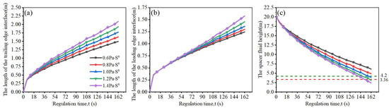
Figure 18.
Effect of the consistency coefficient of the spacer fluid on its interfacial distribution characteristics: (a) effect of spacer fluid’s consistency coefficient on the length of the trailing edge interface; (b) effect of spacer fluid’s consistency coefficient on the length of the leading edge interface; (c) effect of spacer fluid’s consistency coefficient on its height.
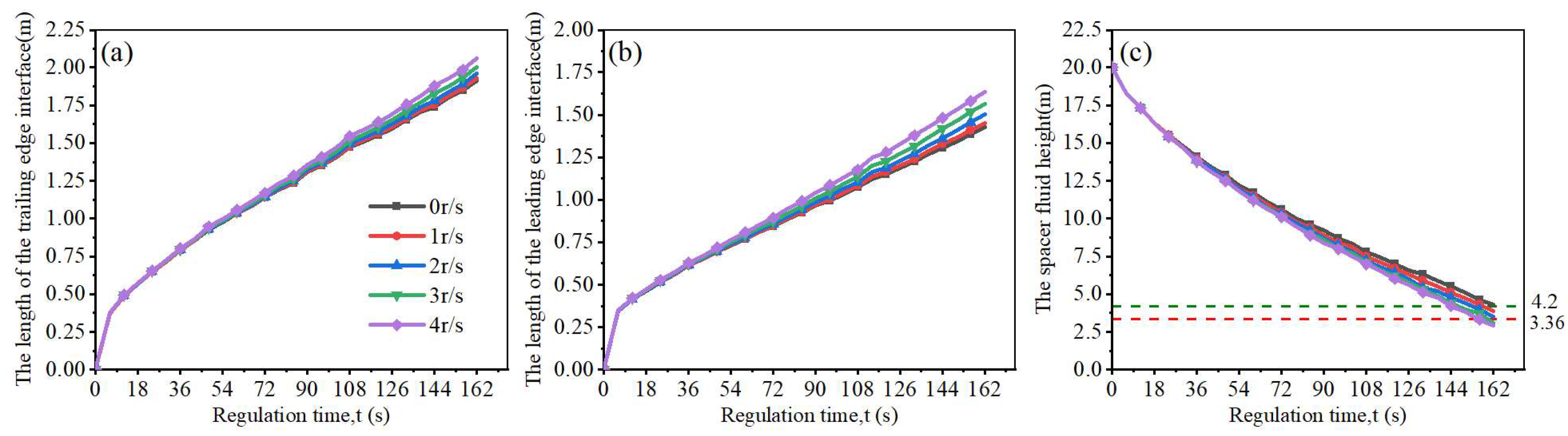
3.4. The Effects of Drill String Rotation Speed on the Stability of the Spacer Fluid Interface
During dual-layer pipe dual-gradient drilling, the fluid in the annulus where the spacer fluid is located makes direct contact with the drill string, so the drill string’s vibration directly impacts the spacer fluid interface. The drilling string, in deepwater drilling, generates many forms of vibration that threaten drilling safety. Stick-slip vibration is one of the main manifestations [40], and the rotation speed of the drilling string has an important influence on stick-slip vibration. Therefore, when considering the impact of drilling string vibration on the stability of the spacer fluid interface, the effect of the drilling string rotation speed was studied first. We adopted the rotation speeds of 0, 1, 2, 3, and 4 r/s for the simulation study. The results are shown in Figure 19.
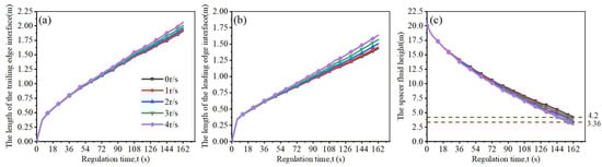
Figure 19.
Effect of the rotation speed of the drill string on the distribution characteristics of the spacer fluid interface: (a) effect of drill string’s rotation speed on the length of the trailing edge interface; (b) effect of drill string’s rotation speed on the length of the leading edge interface; (c) effect of drill string’s rotation speed on the spacer fluid height.
Figure 19 shows that as the drill string’s rotation speed increased, the length of the leading and the trailing edge interfaces increased. The spacer fluid height decreased with the drill string’s rotation speed increase, but the difference was not significant. The spacer fluid interface was stable when the drilling string was not rotating; the spacer fluid interface was relatively stable when the drilling string speed was between 1 r/s and 2 r/s; increasing the speed above 3 r/s caused the interface to become unstable. Bu Yuhuan studied the influence of casing rotation on cementing quality, and the results showed that rotating the casing helped to improve the displacement efficiency, that is, the length of the interface between different fluids will increase [30].
We analyzed the reasons for this phenomenon. As shown in Figure 20, in the tangential velocity cloud map, red represents the maximum, and blue represents the minimum. Therefore, the tangential velocity gradually decreased from the dual-layer pipe to the casing direction. The distribution pattern of the tangential velocity cloud map was consistent in the same cross-section at different rotation speeds. Still, there was a significant difference in the value of tangential velocity. The tangential velocity and the shear rate increased as the rotation speed increased. According to the shear thinning effect of pseudoplastic fluids, the apparent viscosity of the fluid decreases, resulting in an enhanced flow. Therefore, when the rotation speed of the drill string increased within the range of 0–4 r/s, the axial flow velocity of the fluid increased, the inhomogeneity of the axial velocity distribution increased, and the stability of the interface decreased.
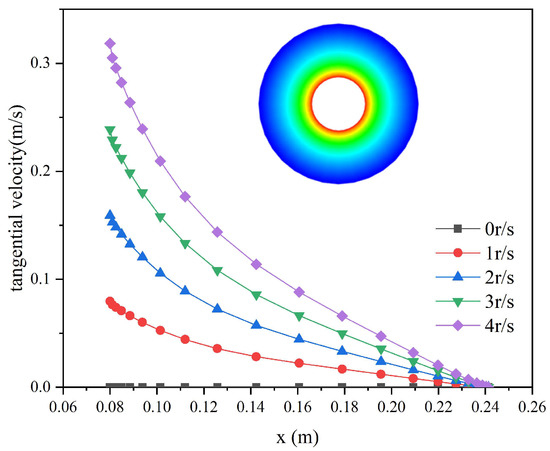
Figure 20.
Fluid tangential velocity distribution and the effect of drill string rotation speed on tangential velocity.
4. Conclusions
In this work, a seawater-spacer fluid-drilling mud annular flow model for dual-layer pipe dual-gradient drilling was established, and an evaluation standard for the stability of the spacer fluid interface was conducted. The computational fluid dynamics method was used to simulate the flow of annular fluid when regulating the bottom hole pressure of 0.2 MPa. We investigated the effects of the flow rate and physical parameters of the spacer fluid and the rotation speed of the drill string on the stability of the spacer fluid interface. The conclusions of this paper can be summarized as follows:
- (1)
- The flow velocity of the annular fluid and the physical parameters of the spacer fluid including the density, liquidity index, and consistency coefficient are the main factors affecting the stability of the spacer fluid interface. In contrast, the drilling mud rotation speed has less influence on the stability of the spacer fluid interface.
- (2)
- During the regulation of pressure in the wellbore, the annular fluid’s flow velocity increases, leading to a rise in the inhomogeneity of the axial velocity distribution and a decrease in interface stability. The spacer fluid interface is stable when the flow velocity is between 0.04 m/s and 0.16 m/s. However, when the flow velocity increases to 0.2 m/s and the spacer fluid height is reduced to just 3 m after regulation, the spacer fluid interface is unstable. In practical engineering applications, we recommend regulating the bottom hole pressure with a low flow rate and maintaining drilling throughout the regulation process. This not only helps to maintain the stability of the spacer fluid interface but also ensures that the dual-layer pipe returns a sufficient drilling mud flow for rock carrying, thus ensuring drilling safety and efficiency.
- (3)
- The influence of the spacer fluid’s density is mainly reflected in its density difference from the seawater and drilling mud. The greater the density difference, the more significant the buoyancy effect, resulting in a smaller length of the spacer fluid’s interface and a more stable interface. The stability of the spacer fluid interface decreases with the increase in its liquidity index and consistency coefficient; when its liquidity index is in the range of 0.5~0.8 and its consistency coefficient is in the range of 0.6~0.8 , the spacer fluid interface is stable. However, when the liquidity index of the spacer fluid increases to 0.9 and the consistency coefficient increases to 1.2~1.4 , the interface becomes unstable.
This study identified the main control factors and their influence patterns on the stability of the spacer fluid interface. It provides a reference for the selection of operational parameters to ensure that seawater and drilling mud do not mix during the whole drilling process, thereby maintaining the stable operation of the dual-layer pipe dual-gradient drilling system.
In the future, the influence of other factors that affect the vibration of the drill string such as the drilling pressure on the spacer fluid interface will be studied based on the research in this paper. Moreover, the effects of the coupling of various factors on the stability of the spacer fluid interface will be investigated in order to obtain the optimal combination of drilling parameters to maintain the stable operation of the dual-gradient pressure system and guide the drilling operations.
Author Contributions
Software, X.L.; Validation, X.L. and Z.L.; Writing—original draft preparation, G.W., X.L. and L.Z.; Writing—review and editing, X.L. and G.W. All authors have read and agreed to the published version of the manuscript.
Funding
This research was funded by the National Key Research and Development Program of China, grant numbers 2018YFC0310201 and 2019YFC0312305, and the Sichuan Provincial Department of Science and Technology Natural Science Fund Innovative Research Group Project, grant number 2023NSFSC1980.
Data Availability Statement
The data that support the findings of this study are available from the corresponding author upon reasonable request.
Conflicts of Interest
The authors declare no conflict of interest.
Nomenclature
| Pb | Bottom hole pressure |
| Density of the seawater, spacer and drilling mud, respectively (kg/cm3) | |
| Height of the seawater, spacer fluid, and drilling mud, respectively (m) | |
| Equivalent density (kg/cm3) | |
| Equivalent well depth (m) | |
| d | Inner diameter of annulus (mm) |
| D | Outer diameter of annulus (mm) |
| A | Cross-sectional area of the annular (m2) |
| Flow difference (L/S) | |
| v | Annular fluid flow velocity (m/s) |
| Static pressure | |
| Gravitational body force | |
| External body forces | |
| Stress tensor | |
| Local mass fraction of each species | |
| Diffusion flux of species | |
| Net rate of production of species via a chemical reaction | |
| Turbulence kinetic energy due to the mean velocity gradients | |
| Turbulence kinetic energy due to buoyancy | |
| Turbulent viscosity | |
| RMR | Riserless Mud Recovery |
| CAML | Controlled annular mud level |
| CAPM | Continuous annular pressure management system |
| ROP | Rate of penetration |
References
- Zhang, G.C.; Qu, H.J.; Zhang, F.L.; Chen, S.; Yang, H.Z.; Zhao, Z.; Zhao, C. Major new discoveries of oil and gas in global deepwaters and enlightenment. Acta Petrolei Sinica 2019, 40, 1–34. [Google Scholar]
- Cohen, J.H.; Stave, R.; Hauge, E.; Molde, D.O. Field Trial of Well Control Solutions with a Dual Gradient Drilling System. In Proceedings of the SPE/IADC Managed Pressure Drilling and Underbalanced Operations Conference & Exhibition, Dubai, United Arab Emirates, 13–14 April 2015. [Google Scholar]
- Yin, Z.; Li, Z.; Huang, X. Scheme optimization of deepwater dual gradient drilling based on the fuzzy comprehensive evaluation method. Ocean Eng. 2023, 281, 114978. [Google Scholar] [CrossRef]
- Myers, G. Ultra-deepwater riserless mud circulation with dual gradient drilling. Sci. Drill. 2008, 6, 48–51. [Google Scholar] [CrossRef]
- Guo, X.; Zhang, Z. Study on the pressure wave velocity model of multiphase fluid in the annulus of dual-gradient drilling. Therm. Sci. 2023, 136. [Google Scholar] [CrossRef]
- Keshavarz, M.; Moreno, R.B. Qualitative analysis of drilling fluid loss through naturally-fractured reservoirs. SPE Drill. Complet. 2023, 1–17. [Google Scholar] [CrossRef]
- Zhang, M.F. Analysis of the current situation and development trend of deepwater drilling technology. China Pet. Chem. Stand. Qual. 2018, 38, 138–139+141. [Google Scholar]
- Waernes, K. Applying Dual Gradient Drilling in Complex Wells, Challenges and Benefits. Master’s Thesis, University of Stavanger, Stavanger, Norway, 2013. [Google Scholar]
- Dual gradient drilling systems. Available online: https://petrowiki.spe.org/Dual_gradient_drilling_systems (accessed on 20 February 2023).
- What Is Riserless Mud Recovery. Available online: https://www.iodp.org/241-12-what-is-riserless-mud-recovery-cohen/file (accessed on 26 February 2023).
- Judge, B.; Hariharan, P.R. Realizing Zero Discharge Riserless Drilling and Annular Pressure Management With a Single Tool. In Proceedings of the Offshore Technology Conference, Houston, TX, USA, 2–5 May 2005. [Google Scholar]
- RMR®—Riserless Mud Recovery. Available online: https://www.enhanced-drilling.com/rmr-solution (accessed on 26 February 2023).
- Stave, R. Implementation of Dual Gradient Drilling. In Proceedings of the Offshore Technology Conference, Houston, TX, USA, 5–8 May 2014. [Google Scholar]
- Ziegler, R.; Sabri, M.S.; Idris, M.R.; Malt, R.; Stave, R. First Successful Commercial Application of Dual Gradient Drilling in Ultra-Deepwater GOM. In Proceedings of the SPE Annual Technical Conference and Exhibition, New Orleans, LA, USA, 30 September–2 October 2013. [Google Scholar]
- Ziegler, R.; Ashley, P.; Malt, R.F.; Stave, R.; Toftevåg, K.R. Successful Application of Deepwater Dual Gradient Drilling. In Proceedings of the IADC/SPE Managed Pressure Drilling and Underbalanced Operations Conference and Exhibition, San Antonio, TX, USA, 17–18 April 2013. [Google Scholar]
- Yin, Z.M.; Chen, G.M.; Wang, Z.X.; Xu, L.B.; Jiang, S.Q. Deepwater subsea mud-lift drilling technology and its application prospects. Drill. Prod. Technol. 2006, 29, 1–3+137. [Google Scholar]
- Lopes, C.A.; Bourgoyne, A.T., Jr. The Dual Density Riser Solution. In Proceedings of the SPE/IADC Drilling Conference, Amsterdam, The Netherlands, 4–6 March 1997. [Google Scholar]
- Han, T.W.; Jiang, H.W.; Yang, G. Classification and research progress of deep water dual gradient drilling technology. Oil Field Equip. 2019, 48, 83–89. [Google Scholar]
- Golsanami, N.; Gong, B.; Negahban, S. Evaluating the effect of new gas solubility and bubble point pressure models on PVT parameters and optimizing injected gas rate in gas-lift dual gradient drilling. Energies 2022, 15, 1212. [Google Scholar] [CrossRef]
- Zhang, J.B. Study on Design and Configuration of Dilution-Based Dual Gradient Drilling System. Master’s Thesis, China University of Petroleum (East China), Dongying, China, 2016. [Google Scholar]
- Halkyard, J.; Anderson, M.R.; Maurer, W.C. Hollow Glass Microspheres: An Option for Dual Gradient Drilling and Deep Ocean Mining Lift. In Proceedings of the Offshore Technology Conference-Asia, Kuala Lumpur, Malaysia, 25–28 March 2014. [Google Scholar]
- Wang, G.R.; Zhong, L.; Liu, Q.Y.; Zhou, S.W. Research on marine petroleum and hydrate development technology based on dual gradient drilling of double-layer pipe. Ocean Eng. Equip. Technol. 2019, 6 (Suppl. S1), 225–233. [Google Scholar]
- Vestavik, O.M.; Thorogood, J.; Bourdelet, E.; Schmalhorst, B.; Roed, J.P. Horizontal Drilling with Dual Channel Drill Pipe. In Proceedings of the SPE/IADC Drilling Conference and Exhibition, The Hague, The Netherlands, 14–16 March 2017. [Google Scholar]
- Tang, Y.; Zhao, P.; Wang, G.R.; Li, X.S.; Fang, X.Y. Horizontal pipe migration law of multiphase mixed slurry in offshore gas hydrate mining. J. Cent. South Univ. (Sci. Technol.) 2022, 53, 1047–1057. [Google Scholar]
- Wang, J.S.; Fu, P.; Hu, X.H.; Gong, C.X.; Deng, S.; Tang, Z.; Yin, W. Distribution law of wellbore temperature in offshore dual-layer DEG. China Pet. Mach. 2022, 50, 51–57. [Google Scholar]
- Savery, M.; Darbe, R.; Chin, W. Modeling Fluid Interfaces During Cementing Using a 3D Mud Displacement Simulator. In Proceedings of the Offshore Technology Conference, Houston, TX, USA, 30 April–3 May 2007. [Google Scholar]
- Wu, Z.Q.; Chen, Z.H.; Zhao, Y.P.; Xue, Y.C.; Wang, C.W.; Xiong, C.; Chen, S.L. Theoretical and experimental study on cementing displacement interface for highly deviated wells. Energies 2023, 16, 733. [Google Scholar] [CrossRef]
- Jung, H.; Frigaard, I.A. Evaluation of common cementing practices affecting primary cementing quality. J. Pet. Sci. Eng. 2022, 208, 109622. [Google Scholar] [CrossRef]
- Choi, M.; Scherer, G.W.; Prudhomme, R.K. Novel methodology to evaluate displacement efficiency of drilling mud using fluorescence in primary cementing. J. Pet. Sci. Eng. 2018, 165, 647–654. [Google Scholar] [CrossRef]
- Bu, Y.H.; Tian, L.J.; Li, Z.B.; Zhang, R.; Wang, C.Y.; Yang, X.C. Effect of casing rotation on displacement efficiency of cement slurry in highly deviated wells. J. Nat. Gas Sci. Eng. 2018, 52, 317–324. [Google Scholar] [CrossRef]
- Chen, Y. Experimental Study of Cementing in Eccentric Horizontal Annulus. Master’s Thesis, China University of Petroleum, Beijing, China, 2016. [Google Scholar]
- Wang, B.Q. Study on Numerical Simulation of Cementing Displacement. Master’s Thesis, China University of Petroleum, Beijing, China, 2019. [Google Scholar]
- Tang, Y.; Yao, J.X.; Wang, G.R.; He, Y.; Sun, P. Analysis of multi-phase mixed slurry horizontal section migration efficiency in natural gas hydrate drilling and production method based on double-layer continuous pipe and double gradient drilling. Energies 2020, 13, 3792. [Google Scholar] [CrossRef]
- Zhang, X.Q.; Ding, D.H.; Zhou, Y.C.; Liu, W. Application of fine managed pressure drilling in near-balance drilling. Spec. Oil Gas Reserv. 2016, 23, 141–143+158. [Google Scholar]
- Zhu, H.Y.; Liu, Q.Y.; Wang, T. Reducing the bottom-hole differential pressure by vortex and hydraulic jet methods. J. Vibroengineering 2014, 16, 2224–2249. [Google Scholar]
- Wang, S.T. Study on Displacement Efficiency of Cementing under Non-uniform Geometric Boundary Conditions. Ph.D. Thesis, Northeast Petroleum University, Daqing, China, 2020. [Google Scholar]
- Shafiei, M.; Kazemzadeh, Y.; Martyushev, D.A.; Dai, Z.; Riazi, M. Effect of chemicals on the phase and viscosity behavior of water in oil emulsions. Sci. Rep. 2023, 13, 4100. [Google Scholar] [CrossRef]
- Kaleem, W.; Tewari, S.; Fogat, M.; Martyushev, D.A. A hybrid machine learning approach based study of production forecasting and factors influencing the multiphase flow through surface chokes. Petroleum 2023. [Google Scholar] [CrossRef]
- Yang, J.W. Research on Improving Cement Injection Displacement Efficiency in Horizontal Sections of Horizontal Wells in Block LX. Master’s Thesis, Yangtze University, Jingzhou, China, 2020. [Google Scholar]
- Ren, K. Research on Characteristics of Drill String Vibration Based on Measurement Parameters of Near Bit. Master’s Thesis, China University of Petroleum, Beijing, China, 2019. [Google Scholar]


Disclaimer/Publisher’s Note: The statements, opinions and data contained in all publications are solely those of the individual author(s) and contributor(s) and not of MDPI and/or the editor(s). MDPI and/or the editor(s) disclaim responsibility for any injury to people or property resulting from any ideas, methods, instructions or products referred to in the content. |
© 2023 by the authors. Licensee MDPI, Basel, Switzerland. This article is an open access article distributed under the terms and conditions of the Creative Commons Attribution (CC BY) license (https://creativecommons.org/licenses/by/4.0/).