Optimizing Photovoltaic Power Production in Partial Shading Conditions Using Dandelion Optimizer (DO)-Based MPPT Method

Abstract

This research proposes the dandelion optimizer (DO), a bioinspired stochastic optimization technique, as a solution for achieving maximum power point tracking (MPPT) in photovoltaic (PV) arrays under partial shading (PS) conditions. In such scenarios, the overall power output of the PV array is adversely affected, with shaded cells generating less power and consuming power themselves, resulting in reduced efficiency and local hotspots. While bypass diodes can be employed to mitigate these effects by redirecting current around shaded cells, they may cause multiple peaks, making MPPT challenging. Therefore, metaheuristic algorithms are suggested to effectively optimize power output and handle multiple peaks. The DO algorithm draws inspiration from the long-distance movement of a dandelion seed, which relies on the force of the wind. By utilizing this bioinspired approach, the DO algorithm can successfully capture the maximum power point (MPP) under different partial shading scenarios, where traditional MPPT algorithms often struggle. An essential contribution of this research lies in the examination of the performance of the proposed algorithm through simulation and real-time hardware-in-the-loop (HIL) results. Comparing the DO algorithm with the state-of-the-art algorithms, including particle swarm optimization (PSO) and cuckoo search (CS), the DO algorithm outperforms them in terms of power tracking efficiency, tracking duration, and the maximum power tracked. Based on the real-time HIL results, the DO algorithm achieves the highest average efficiency at 99.60%, surpassing CS at 96.46% and PSO at 94.74%. These findings demonstrate the effectiveness of the DO algorithm in enhancing the performance of MPPT in PV arrays, particularly in challenging partial shading conditions.

1. Introduction

In the past decade, there has been a significant global focus on the study of renewable energy sources. This emphasis has arisen as a response to pressing issues such as increasing energy consumption, dwindling fossil fuel reserves, and the urgent necessity to mitigate environmental degradation caused by global warming. These energy sources include wind, solar, geothermal, hydro, and biomass, each with its unique features and merits. Among these alternatives, solar energy, specifically photovoltaic (PV) panels, has gained significant traction in recent years due to its environmentally friendly nature, high safety standards, cleanliness, lack of noise pollution, and low maintenance requirements [1,2,3,4]. PV systems are commonly categorized into two groups based on their intended use. The first group consists of utility-shared PV systems, which encompass hybrid power systems, grid-tied systems, power plants, and various interconnected applications. The second group comprises stand-alone PV systems, which are utilized to power electrical pumps, electric vehicles (EVs), space applications, and street lights, as well as other independent devices [5,6,7].

The effectiveness of PV energy systems is significantly affected by partial shading (PS) environments, which emerge as a prominent challenge due to the outdoor installation of these systems. The efficiency of PV systems can be greatly influenced by temperature and irradiance levels. These factors are very important in determining the properties of PV systems, as observed in their I-V (current–voltage) and P-V (power–voltage) curves. Of particular importance is the presence of a maximum power point (MPP), which represents the optimal operating point where the highest output is attained. However, partial shading brought on by factors such as trees, buildings, clouds, dust deposition, etc., can result in hotspot formation on shaded portions of PV panels, leading to reduced performance [8,9]. To tackle this problem, a commonly employed approach involves incorporating bypass diodes into specific cells within the series circuit. The effect of partial shading is lessened because of the contribution of these diodes, which play an important function in the process. However, the presence of bypass diodes can result in the formation of both a global maximum power point (GMPP) and many local maximum power points (LMPPs) inside the I-V and P-V curves. It is essential to be aware that taking electricity from the LMPPs can considerably reduce the overall efficiency of the PV system. The term “maximum power point tracking” (MPPT) describes the process of squeezing the most possible power out of a PV system while maintaining precise tracking of the GMPP [5,8,10]. A PV module, MPPT controller, boost converter, and load are the essential components of a typical stand-alone PV system. The DC-DC boost converter serves as a conduit between the PV panel and the load, making it possible to exercise precise command over the process of MPPT. The duty cycle is the control variable, and it is an extremely important component in the process of precisely regulating the operation of the converter [11].

Techniques for MPPT are categorized according to a variety of criteria, including the degree of difficulty involved in putting them into practice, the structure of their algorithms, and the resources that are needed [5]. Conventional MPPT algorithms have found extensive application in maximizing the power output of PV systems. These include perturb and observe (P&O) [12], hill climbing (HC) [13], incremental conductance (INC) [14], fractional short-circuit current (FSCC) [15], and fractional open-circuit voltage (FOCV) [16]. The P&O, INC, and FOCV algorithms have gained popularity in MPPT applications due to their user-friendly nature. However, the P&O and INC algorithms suffer from two significant drawbacks. Firstly, they exhibit poor tracking performance in rapidly changing weather conditions. Secondly, these algorithms can lead to increased power loss as a result of significant oscillations. The open-circuit voltage of the solar panel is rated as part of the operation of the algorithm that is based on FOCV. However, this approach can lead to temporary power loss during variations in irradiance levels. The FSCC algorithm faces similar issues. Moreover, these methods are module-dependent and may be less efficient because they require knowledge of PV module properties and manufacturing requirements [17]. Nevertheless, these algorithms are renowned for their dependability and straightforward structure, which allow for effective tracking under constant solar irradiation. However, when there are several MPPs, they can quickly become trapped at an LMPP, which frequently leads to weak performance [3].

The conventional approaches may not be sufficient to effectively handle PSCs, thus necessitating the need for more advanced approaches. Several studies have been conducted on soft computing techniques in this context, including fuzzy logic controllers (FLCs) [18] and artificial neural networks (ANNs) [19]. In some of these studies, FLCs have been used to improve the effectiveness and dependability of MPP tracking controllers that are functioning in both normal and PS situations. For instance, a novel three-input, one-output FLC-based MPPT technique with a beta parameter was proposed in [20] to address partial shading conditions (PSCs). This approach simplifies the fuzzy rule membership functions, extends its applicability to wider operating conditions, and reduces the reliance on familiarity with the system beforehand. The FLC-based MPPT technique is particularly effective for solar PV systems, with a high convergence rate and very few oscillations [21]. However, when exposed to abrupt variations in temperature and light, the FLC-based method may experience inaccurate membership functions. Artificial intelligence (AI)-based solutions that do not need precise parameters or system expertise have been proposed as a solution to this. Even though they need a sizable amount of training data, artificial neural networks (ANNs) have been shown to be an effective tool for managing complex nonlinear systems [19].

However, in recent years, a novel category of MPPT controllers utilizing metaheuristic algorithms has gained unexpected popularity. These controllers have a reputation for being adaptable, using a gradient-free approach, and being able to avoid local optima, all of which are useful for dealing with difficult PS conditions. Particle swarm optimization (PSO) has received significant attention in the literature due to its usefulness in efficiently optimizing stochastic functions. However, the traditional PSO approach has drawbacks, such as a reliance on random coefficients, constant particle velocity, slow convergence speed leading to long tracking times, and high computational cost due to memory requirements for recording particle movement in microcontrollers. To overcome these challenges, various studies have proposed modifications to enhance the performance of standard PSO. The study described in [22] explores an enhanced PSO algorithm that uses a randomization factor (α) that varies with iterative time to minimize computation burden and improve performance when contrasted with the conventional PSO algorithm. In [23], an MPPT algorithm based on accelerated particle swarm optimization (APSO) is presented. The P&O MPPT algorithm is incorporated into the APSO algorithm. In this algorithm, the particle that possesses the best fitness value (i.e., PV power) is the one that becomes perturbed. As a result, the best particle is accelerated, enabling it to converge more swiftly towards the GMPP. Nevertheless, despite the proposed improvements, the issue of high time constraints and computational burden persist to a significant extent. The implementation of the cuckoo search (CS) optimization method in [24] updates the particle positions using the Levy flight function. However, this approach can result in large fluctuations in output voltage transients due to the intrinsic nature of long and short flights produced by the Levy flight function. Article [25] demonstrates how the CS algorithm is implemented for MPPT with a modified Levy flight function under various irradiance and temperature circumstances. The operation of CS is compared with other methods, such as INC and ANN, and it is demonstrated that CS outperforms these methods in terms of MPPT performance. In [26], the utilization of the artificial bee colony (ABC) algorithm is proposed for the MPPT of a PV system incorporating a DC-DC converter. In [27], a novel MPPT control method is presented, employing moth flame optimization (MFO), and evaluated under diverse irradiance levels and partial shading scenarios. When compared to other MPPT techniques, the MFO-based MPPT method exhibits a longer convergence time but demonstrates greater effectiveness in capturing global maxima. The study examines the grey wolf optimizer (GWO), as presented in [28], and observes that despite its high power tracking efficiency, it suffers from longer settling time owing to the need for larger populations to achieve higher efficiency. In [29], the comfort zone parameter is used by the grasshopper optimization (GHO) technique to uphold an equilibrium between the stages of exploitation and exploration of the optimization process. However, the nonlinear parameter must be precisely tuned to produce the best results. Additionally, Ref. [30] compares seven metaheuristic training algorithms for neuro-fuzzy training in MPPT. The algorithms used are PSO, harmony search (HS), CS, ABC, bee algorithm (BA), differential evolution (DE), and flower pollination algorithm (FPA) to determine the parameters of neuro-fuzziness for MPPT. The study evaluates different neuro-fuzzy structures, membership functions, and control parameter values to achieve effective MPPT. However, the study only uses simulation data from a PV system, and the performance of algorithms in real-world scenarios is not tested.

In general, PSO offers several advantages, including its ability to efficiently explore complex search spaces and its simple implementation. However, one of its drawbacks is that it may become stuck in local optima, leading to suboptimal solutions. Additionally, the convergence rate of PSO can be slow, particularly in high-dimensional problems, and it may suffer from premature convergence. On the other hand, CS is known for its effective exploitation and exploration capabilities, making it suitable for global optimization tasks. Nevertheless, CS has its share of disadvantages. One major issue is its heavy reliance on randomization, which can lead to unpredictable variations in the output signal, affecting the convergence and stability of the optimization process. Moreover, CS may exhibit slower convergence rates compared to other algorithms. The ABC and MFO algorithms share a common characteristic of choosing candidate solutions probabilistically. While this stochastic nature allows for the exploration of the search space, it can lead to undesirable oscillations in the output. These oscillations at the GMPP can result in significant power losses and decreased energy production in the PV system. Consequently, in scenarios where a smooth and stable output is crucial, such as during continuous MPPT tracking, ABC and MFO may fall short. The GWO algorithm excels in clear sky conditions as it successfully follows the GMPP. However, it may encounter challenges in cloudy PV system conditions. Gray wolves move slowly in the search space and require more iterations as the tuning parameter decreases with time. This constraint can lead to the LMPP trap, where the algorithm may become stuck in local optima, causing delayed GMPP tracking and reduced efficiency in capturing the optimal power output. On the other hand, the GHO algorithm demonstrates promising abilities in monitoring the GMPP, even under PSCs. It can effectively adapt to changing conditions and maintain stability in the output power. However, the presence of tuning constraints in GHO may introduce casual oscillations in the output power at the GMPP. While these oscillations are not as severe as the undesirable fluctuations seen in ABC and MFO, they can still impact the overall power production and introduce some power losses.

Overall, the choice of optimization algorithm for MPPT in PV systems should be considered carefully, considering the specific environmental conditions and system requirements. Therefore, this research presents a novel method for PV-system MPPT control that overcomes the drawbacks of earlier methods. The approach uses a swarm intelligence bio-inspired metaheuristic algorithm called dandelion optimizer (DO) [31] to improve GMPP tracking. The DO algorithm stands out with its unique approach to modeling dandelion seed flight dynamics in a three-stage process: rise, descent, and landing. During the rising stage, random trajectories are integrated to facilitate easy adaptation to different weather conditions. As the algorithm progresses to the descending stage, Brownian motion trajectory is utilized, while the landing stage employs a linear increasing function combined with Levy flight. This clever combination of trajectory patterns enables DO to achieve a harmonious balance between exploration and exploitation. This balance significantly enhances the precision and effectiveness of locating the GMPP in various weather conditions and dynamic environments. By introducing this novel modeling approach, DO emerges as a promising and innovative solution for MPPT in PV systems. It exhibits adaptability to changing conditions and efficient power tracking, making it a reliable and efficient choice for optimizing energy harvesting in PV systems.

When examining existing approaches such as PSO and CS, the DO method stands out due to its numerous advantages. One notable benefit of DO is its superior productivity, speed, simplicity, and stability, especially in monitoring steady-state activities. Unlike PSO and CS, which may introduce random fluctuations at the GMPP due to their reliance on random numbers, DO excels in optimizing continuous search spaces without such disturbances. Another significant advantage of DO is its remarkable ability to track and settle at the GMPP swiftly under rapidly changing PSCs. Compared to PSO and CS, DO outperforms by delivering faster convergence and ensuring that the optimal solution is reached efficiently. In summary, the DO-based MPPT technique outshines alternative strategies such as PSO and CS in multiple aspects. Its advantages include higher productivity, speed, simplicity, and stability, particularly when dealing with steady-state activities. Moreover, the ability of DO to optimize continuous search spaces without introducing random fluctuations sets it apart from PSO and CS. By eliminating the undesirable effects of random interactions, DO ensures more reliable and faster convergence, making it a promising optimization approach for a wide range of practical applications.

The remaining parts of this work are organized in the following manner. Section 2 includes an overview of the PV system modeling and the effects of PS conditions. Section 3 elaborates on the proposed DO-based MPPT technique and its functioning as an MPPT algorithm. Section 4 discusses four different cases to validate the proposed technique and evaluate the performance of DO under rapidly changing conditions. Section 5 presents the real-time analysis results acquired by the Typhoon hardware-in-the-loop (HIL) 402 emulator. Finally, in Section 6, the paper concludes.

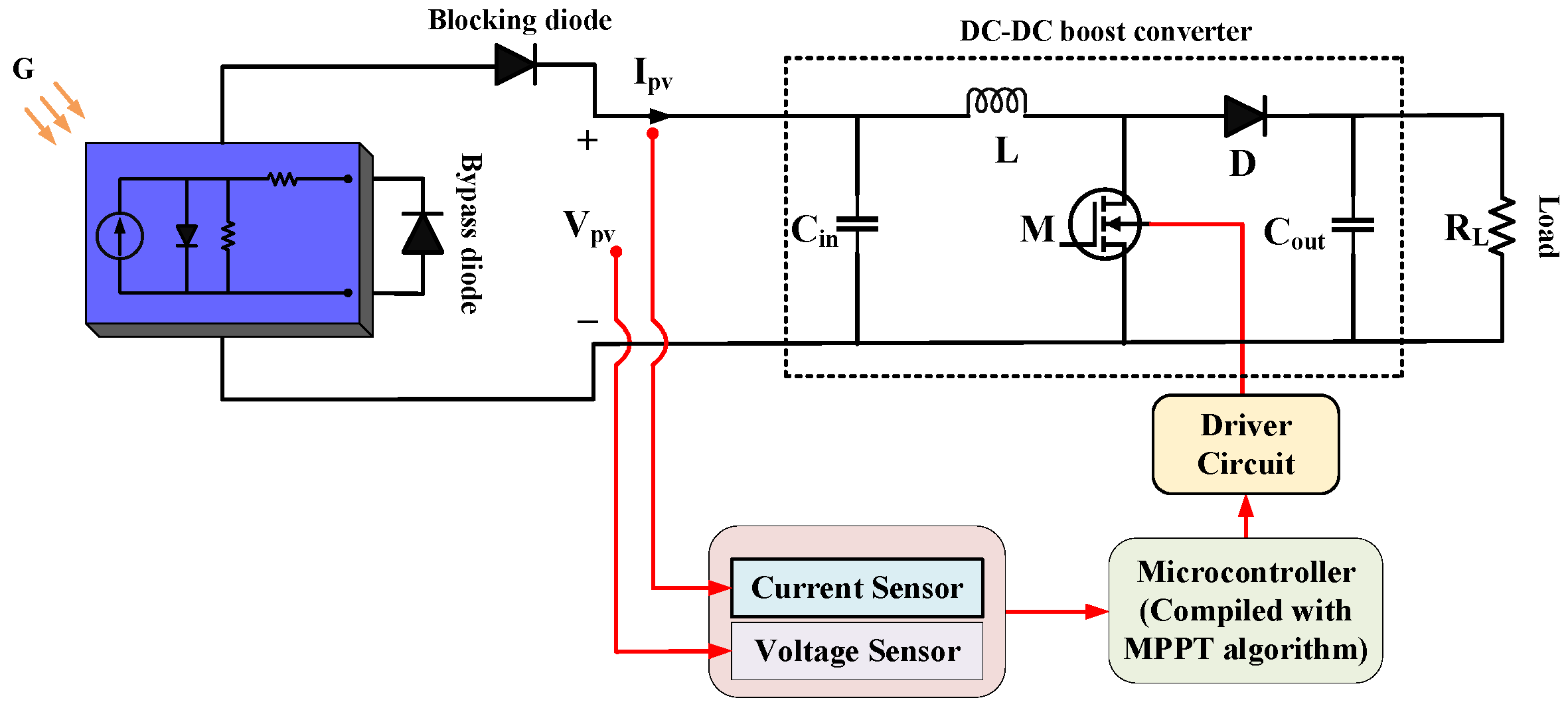
2. Modeling of PV Cells and Analysis of Partial Shading Conditions

This section is dedicated to the mathematical modeling of a PV module by employing a model of a PV cell consisting of a single diode. In addition to this, it digs into the explanation of the partial shading condition, which makes it possible to evaluate how effective the proposed solution is. The use of a DC-DC boost converter as a connection point between the PV array and the load, which enables the implementation of the MPPT approach, is depicted in Figure 1.

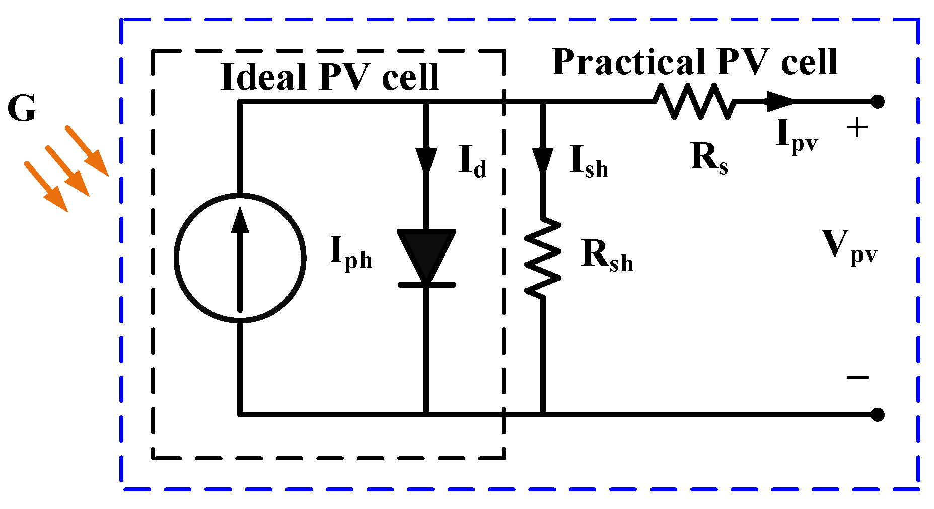
2.1. Single Diode Model of PV Cell

A PV cell consists of an electricity-generating light source, a parallel-connected diode, and a series resistance. Commonly, these PV cells are bundled into PV modules, which can be linked in series or parallel to generate the desired power output. A DC source with an anti-parallel diode can constitute the perfect PV cell [3]. However, to create a more practical model, resistances such as series resistance $(R_s)$ and shunt resistance $(R_{sh})$ need to be included, as shown in Figure 2.

The mathematical expression for a practical single-diode model is given by Equation (1).

$$I_{pv}=N_p{I}_{ph}-N_p{I}_{sat}\times \left[\exp \left(\frac{e}{n{k}_B{T}_o} \left(\frac{V_{pv}}{N_s}+\frac{R_s{I}_{pv}}{N_p}\right)\right)-1\right]-\left[\frac{\frac{N_p{V}_{pv}}{N_s}+\left(R_s{I}_{pv}\right)}{R_{sh}}\right]$$

(1)

where:

• $I_{pv}$: PV output current, $A$.
• $I_{ph}$: photocurrent of PV cell, $A$.
• $I_{sat}$: reverse PV cell saturation current, $A$.
• $V_{pv}$: PV output voltage, $V$.
• $N_p$: number of parallel PV cells.
• $N_s$: number of PV cells in series.
• $e$: electron charge, $1.60217733\times {10}^{-19} \mathrm{C}$.
• $n$: p-n junction diode ideality factor, $1<n<5$.
• $k_B$: Boltzmann’s constant, $1.380658\times {10}^{-23} \mathrm{J}/\mathrm{K}$.
• $T_o$: absolute operating temperature, $K$.

The photocurrent generated, denoted as $I_{ph}$, is determined by the level of solar radiation and can be expressed as Equation (2).

$$I_{ph}=I_{sc}+\left[K_i\times \left(T_o-T_{STC}\right)\times \left(\frac{G}{G_{STC}}\right)\right]$$

(2)

where:

• $I_{sc}$: short-circuit current at ${\mathrm{V}}_{\mathrm{pv}}=0$.
• $K_i$: temperature coefficient of short-circuit current, $\mathrm{A}/\mathrm{K}$.
• $T_{STC}$: the temperature at standard test conditions, $298.15 \mathrm{K}$.
• $G$: PV cell irradiance, $\mathrm{W}/{\mathrm{m}}^2$.
• $G_{STC}$: standard irradiance for testing purposes, $1000 \mathrm{W}/{\mathrm{m}}^2$.

Additionally, Equation (3) demonstrates that the saturation current $(I_{sat})$ of the PV cell is temperature-dependent and subject to variation.

$$I_{sat}=I_{rs}\times {\left(\frac{T_o}{T_{STC}}\right)}^3\times \exp \left[\frac{e{E}_g}{n{k}_B}\left(\frac{1}{T_{STC}}-\frac{1}{T_o}\right)\right]$$

(3)

where:

• $I_{rs}$: reverse saturation current of the diode, $\mathrm{A}$.
• $E_g$: band-gap energy of the semiconductor material utilized in the PV cell, $\mathrm{J}$.

Equations (1)–(3) illustrate the interdependence of solar irradiation and temperature on the current generated by the PV array.

Achieving optimal efficiency in PV systems necessitates operating at the MPP, which is influenced by environmental factors including temperature and irradiance. Figure 3a,b depict the relationships between power–voltage (P-V) and current–voltage (I-V) at various temperatures, while Figure 4a,b demonstrate the same relationship at varying levels of solar irradiance. Increased solar irradiance leads to a higher MPP, whereas higher temperatures result in a lower MPP.

2.2. Partial Shading Phenomenon

To increase power production, PV modules are often connected in both series and parallel configurations. However, when instances of partial shadowing brought by factors such as cloud cover or shade from trees or buildings, certain panels may operate as loads due to uneven levels of irradiance. This mismatch effect can lead to the formation of hotspots. To mitigate these effects, bypass diodes are employed, resulting in several peaks with P-V and I-V characteristics.

Figure 5a illustrates that the P-V and I-V curves exhibit a single MPP when all solar panels receive an identical irradiance level of 1000 W/m². Conversely, Figure 5b represents the scenario of partial shading (PS), where the P-V and I-V curves demonstrate a single GMPP and multiple LMPPs due to varying irradiance values of 1000 W/m², 700 W/m², 600 W/m², and 400 W/m² across the solar panels. In instances of partial shade, the P-V curve comprises numerous LMPPs and just one GMPP. To harvest the maximum amount of solar energy, the PV system must operate at the GMMP. Therefore, a sophisticated MPPT control is necessary to ensure optimal power output despite changes in weather conditions and nonuniform irradiance levels.

3. Dandelion Optimizer-Based MPPT Technique

In this study, a unique bio-inspired meta-heuristic optimization technique called the dandelion optimization (DO) algorithm [31] is utilized. The dandelion, known scientifically as Herba taraxaci, is a perennial Asteraceae plant. It is possible for these herbaceous plants to grow to a height exceeding 20 cm, and they are characterized by their inflorescence-shaped heads. Dandelion seeds typically comprise an achene, a beak, and several crested hairs. The DO algorithm is inspired by the behavior of dandelions, specifically their ability to disperse their seeds over long distances using the wind.

The dispersion of dandelion seeds is primarily influenced by two factors: wind speeds and weather conditions. The velocity of the wind determines the distance that a seed can travel, either over long or short distances. Meanwhile, weather conditions impact the ability of the seed to disperse and grow in nearby or distant areas. The journey of dandelion seeds can be categorized into three stages, as explained below.

Stage 1—Rising stage: The dragging force created by sunny and windy weather causes the dandelion seed to spin and ascend during the rising stage. However, there are no eddies above the seeds when it is raining, which limits their ability to disperse.

Stage 2—Descending stage: The descending stage follows the rising stage, during which the seed descends after reaching a certain height.

Stage 3—Landing stage: The seed eventually lands at random during the landing stage under the influence of the wind and weather, where it can develop into a new dandelion.

3.1. Dandelion Optimization (DO) Algorithm

Dandelions propagate their population through a three-stage process of seed transmission to the succeeding generation, as elaborated in this subsection.

3.1.1. Rising Stage

During the upward stage, dandelion seeds must attain a specific altitude to disperse from the parent plant. Wind speed and air humidity are two of the factors affecting the height the seeds can attain. This stage is characterized by two distinct weather conditions, as follows.

Case 1—Clear day: When the weather is clear, wind speeds follow a lognormal distribution $(\ln Y)$. This distribution causes the random numbers to be more widely dispersed along the $Y$-axis, thereby increasing the probability of dandelion seeds traveling to distant areas. Consequently, exploration is a vital aspect that the algorithm focuses on under these circumstances. Strong winds cause dandelions to fly higher and scatter their seeds farther. The vortices above the dandelion seeds adjust as the wind speed varies to let the seeds flow upward in spiral fashion. This phenomenon is described by the mathematical expression given in Equation (4).

$$D_{t+1}=D_t+\alpha \times u_x\times u_y\times \ln y\times \left(D_s-D_t\right)$$

(4)

where:

• $D_t$: position of a dandelion seed in the t^th iteration.
• $D_{t+1}$: position of a dandelion seed in the (t+1)^th iteration.
• $\alpha$: step size parameter.
• $u_x$: lift coefficient in the horizontal direction.
• $u_y$: lift coefficient in the vertical direction.
• $\ln Y$: lognormal distribution.
• $D_s$: random starting position of the dandelion seed.

Equation (5) presents the formula for the position generated at random.

$$D_s=rand\times \left(D_{max}-D_{min}\right)+D_{min}$$

(5)

where $rand$ generates a random number from a uniform distribution between 0 and 1.

The formula for the lognormal distribution $\ln Y$ is given by Equation (6):

$$\ln Y=\{\begin{array}{c}\frac{1}{y\sqrt{2\pi }}ex{p}^{\left(-\frac{1}{2{\sigma }^2}{\left(\ln y\right)}^2\right)} y\ge 0\\ 0^{ } y<0\end{array}$$

(6)

The lognormal distribution is a notation with a mean $\left(\mu \right)$ of 0 and a variance $({\sigma }^2)$ of 1. The variable $y$ represents the standard normal distribution $N\left(0,1\right)$.

The variability induced by the $\alpha$ parameter instructs the algorithm to start with a global search and then shift to a local one. This approach aids in achieving precise convergence after performing an exhaustive global search. The mathematical formula for this parameter is Equation (7).

$$\alpha =rand\times \left(\frac{1}{t_{max}{}^2}{t}^2-\frac{2}{t_{max}}t+1\right)$$

(7)

The coefficients $u_x$ and $u_y$ are obtained using Equation (8).

$$\begin{array}{c}{u}_x=r\times \cos \theta \\ u_y=r\times \sin \theta \end{array}$$

(8)

Here, the random parameter $r$ is given as Equation (9).

$$\begin{array}{cc}r=\frac{1}{{\mathrm{e}}^{\theta }}& \theta ϵ\end{array}\left[-\pi ,\pi \right]$$

(9)

Case 2—Rainy day: On rainy days, the upward movement of dandelion seeds with the wind is hindered by factors such as air resistance, humidity, and other climatic circumstances. As a result, the seeds rely on local neighborhoods for survival, as described by the mathematical expression in Equation (10).

$$D_{t+1}=D_t\times K$$

(10)

The parameter $K$ regulates the local search range of a dandelion, gradually approaching 1 towards the end of the iteration. This modification guarantees the population converges on the ideal search agent. The domain is calculated using Equation (11).

$$K=1-rand\times q$$

(11)

where $q$ is given as Equation (12).

$$q=\frac{1}{t_{max}{}^2-2t_{max}+1}{t}^2-\frac{2}{t_{max}{}^2-2t_{max}+1}t+1+\frac{1}{t_{max}{}^2-2t_{max}+1}$$

(12)

To summarize, the mathematical formulation for dandelion seeds during the rising stage is given by Equation (13).

$$D_{t+1}=\{\begin{array}{c}{D}_t+\alpha \times u_x\times u_y\times \ln y\times \left(D_s-D_t\right) randn<0.5\\ D_t\times K else\end{array}$$

(13)

To dynamically control the balance between exploitation and exploration, the DO algorithm utilizes a normal distribution of random numbers $\left(randn\right)$. A cutoff point of 0.5 is set to increase the global search orientation of the algorithm. As a result, the first step of iterative optimization can use dandelion seeds to explore the whole search space, giving the later phases of the process the right direction.

3.1.2. Declining Stage

During the descent stage of the DO algorithm, exploration is emphasized, with dandelion seeds descending steadily to a specific distance. To replicate their travel trajectory and enable individuals to cover larger search communities in iterative updates while maintaining a normal distribution for each change, Brownian motion is used. This aids population development towards promising communities. Equation (14) provides the relevant mathematical expression.

$$D_{t+1}=D_t-\alpha \times {\beta }_t\times \left(D_{mean\_t}-\alpha \times {\beta }_t\times D_t\right)$$

(14)

where:

• ${\beta }_t$: Brownian motion derived from the normal distribution.
• $D_{mean\_t}$: average position of the seeds during the t^th iteration.
• $D_{mean\_t}$ is computed using Equation (15).

$$D_{\mathit{mean\_t}}=\frac{1}{pop}\sum _{i=1}^{pop}{D}_i$$

(15)

3.1.3. Land Stage

During this phase of the DO algorithm, a focus is placed on exploitation. After the initial two phases, the dandelion seed selects a random landing location in the hopes of converging towards the global optimal solution. The optimal position is one where dandelion seeds have the best chance of surviving. Search agents utilize the information acquired from the present elite to their benefit, allowing them to converge accurately towards the global optimum in their immediate vicinity. Through the process of population evolution, the global optimal solution can be ultimately achieved. Equation (16) expresses this behavior.

$$D_{t+1}=D_{elite}+levy\left(\lambda \right)\times \alpha \times \left(D_{elite}-D_t\times \delta \right)$$

(16)

where:

• $D_{elite}$: optimal position of the dandelion seed in the t^th iteration.
• $\delta :$ linearly increasing function that ranges from 0 to 2.
• $levy\left(\lambda \right)$: Levy flight function.
• $\delta$ is calculated using Equation (17).

$$\delta =\frac{2t}{t_{max}}$$

(17)

The Levy flight function is calculated using Equation (18).

$$l\mathrm{e}vy\left(\lambda \right)=s\times \frac{w\times \rho }{{\left|m\right|}^{\frac{1}{\phi }}}$$

(18)

In Equation (18), $\phi$ denotes the variance $\left(0\le \phi \le 2\right),$ which is set to 1.5, while $s$ is a constant fixed at 0.01. Both $w$ and $m$ are random numbers ranging from 0 to 1. The mathematical expression for $\rho$ is provided in Equation (19).

$$\rho =\left[\frac{\Gamma \left(1+\phi \right)\times \sin \left(\frac{\pi \phi }{2}\right)}{\Gamma \left(\frac{1+\phi }{2}\right)\times \phi \times 2^{\left(\frac{\phi -1}{2}\right)}}\right]$$

(19)

The behavior of dandelion seeds under various weather conditions is depicted in Figure 6a. During clear weather, dandelion seeds are updated with geographical information chosen at random to encourage exploration. The movement vector is influenced by the eddy above the seed, which spirals in the direction of motion by multiplying the $u_x$ and $u_y$ components. In the second instance, the neighborhood is exploiting dandelion seeds in all directions. In Figure 6b, dandelion seeds are shown to regenerate during their descent. The global search trajectory of Brownian motion is also shown in the figure. The population can search the area close to the global optimum owing to the irregular migration, which helps them avoid the local extremum. Figure 6c demonstrates how the search agent is updated gradually as it moves closer to the final, global optimal answer. During this stage, individuals undergo a linear rising function to prevent excessive exploitation. To replicate the magnitude of individual movement steps, the Levy flight coefficient is applied.

3.2. Execution of DO Algorithm for MPPT

The application of the DO algorithm in MPPT involves specific restrictions and modifications to ensure its effective and accurate operation in PV systems.

• Duty Ratio Initialization and Restrictions: The duty ratios in the DO algorithm represent the control signals transmitted to the converter, akin to dandelion seeds in the natural analogy. To begin the optimization process, the duty ratios must be initialized within a certain search space, which is limited by the maximum value $\left(D_{max}=0.9\right)$ and the minimum value $\left(D_{\min }=0.1\right)$. The reason for these restrictions is to confine the optimization to a safe and feasible range of duty ratios that do not cause instability or exceed the operational limits of the converter. This ensures that the algorithm starts with reasonable values for power conversion, avoiding any unsafe or impractical configurations.
• Iterative Optimization Process: The DO algorithm proceeds with an iterative optimization process, consisting of three stages: rising, descending, and landing. During the rising stage, the duty ratios undergo random trajectories, allowing for a broad exploration of the search space to identify potential optimal points. In the descending stage, the Brownian motion trajectory is employed to refine the optimization process, focusing on promising regions in the search space. Finally, the landing stage utilizes a linear increasing function with Levy flight to fine-tune the duty ratios, aiming to converge towards the GMPP.
• Obtaining the Optimum Duty Ratio: Through the iterative process, the DO algorithm continuously updates the positions of the duty ratios until it reaches a point of convergence, where the optimum duty ratio representing the GMPP is identified. This duty ratio is then sent to the converter, adjusting the power conversion to operate at the optimal power output of the PV system.

Figure 7 is a flowchart that showcases the step-by-step operation of the DO algorithm under PS conditions. The flowchart provides a visual representation of how the algorithm progresses through the different stages, updating duty ratios, and ultimately obtaining the GMPP.

4. Simulation Results and Analysis

The simulation arrangement for the DO-MPPT control-based PV system inspired by biological processes comprises a PV panel array, a boost converter, and a stand-alone load. The MPPT controller adjusts the duty cycle $\left(D\right)$ of the boost converter by taking $\left(I_{pv}\right)$ and $\left(V_{pv}\right)$ as inputs to generate the duty cycle $\left(D\right)$. The electrical properties of the PV panel are given in

Table 1. Electrical characteristics of PV array.

Parameters	Values
Number of PV modules in series	4
$\mathrm{Number} \mathrm{of} \mathrm{series} \mathrm{connected} \mathrm{cells} \mathrm{per} \mathrm{module} (N_s)$	72
$\mathrm{Maximum} \mathrm{operating} \mathrm{power} (P_{mp})$	87.348 W
$\mathrm{Maximum} \mathrm{operating} \mathrm{current} (I_{mp})$	5.02 A
$\mathrm{Maximum} \mathrm{operating} \mathrm{voltage} (V_{mp})$	17.4 V
Short-circuit current $(I_{sc})$	5.34 A
Open-circuit voltage $(V_{oc})$	21.7 V
$\mathrm{Temperature} \mathrm{coefficient} \mathrm{of} I_{sc} (K_i)$	0.075%/°C
$\mathrm{Temperature} \mathrm{coefficient} \mathrm{of} V_{oc} (K_v)$	−0.37501%/°C
$\mathrm{Photogenerated} \mathrm{current} (I_{ph})$	5.3624 A
$\mathrm{Diode} \mathrm{saturation} \mathrm{current} (I_{sat})$	3.052 × 10−10 A
$\mathrm{Diode} \mathrm{ideality} \mathrm{factor} \left(n\right)$	0.12439
$\mathrm{Series} \mathrm{resistance} (R_s)$	79.3172 Ω
$\mathrm{Shunt} \mathrm{resistance} (R_{sh})$	0.081018 Ω

, and the PV system is precisely modeled in MATLAB/Simulink 2020a using research findings from [32,33,34]. The simulation is performed on a host computer with an Intel^® Core™ i5-10210U CPU running at 1.60 GHz and 8 GB of RAM. The values of the components used in the simulation are shown in

Table 2. Component specifications in the simulation.

Components	Values
$\mathrm{Power} \mathrm{rating} \mathrm{of} \mathrm{the} \mathrm{PV} \mathrm{module} \left(P_{pv}\right)$	21.837 W
$\mathrm{Input} \mathrm{capacitance} \left(C_{in}\right)$	$47 \mathsf{\mu }\mathrm{F}$
$\mathrm{Output} \mathrm{capacitance} \left(C_{out}\right)$	$470 \mathsf{\mu }\mathrm{F}$
$\mathrm{Inductor} \left(L\right)$	$1.478 \mathrm{mH}$
$\mathrm{Switching} \mathrm{frequency} \left(f\right)$	$20 \mathrm{kHz}$
$\mathrm{Load} \left(R_L\right)$	10 Ω

and

Table 3. Parameters of PSO, CS and DO for MPPT.

Parameters	PSO	CS	DO
$\mathrm{Number} \mathrm{of} \mathrm{particles} \left(pop\right)$	4	4	4
$\mathrm{Maximum} \mathrm{number} \mathrm{of} \mathrm{iterations} \left(t_{max}\right)$	10	10	10
$\mathrm{Social} \mathrm{parameter} \left(c2\right)$	1.2	$-$	$-$
$\mathrm{Cognitive} \mathrm{parameter} \left(c1\right)$	1.6	$-$	$-$
$\mathrm{Inertia} \mathrm{weight} \left(w\right)$	0.4	$-$	$-$
$\mathrm{Step} \mathrm{size} \left(\alpha \right)$	$-$	0.8	$-$
$\mathrm{Variance} \left(\phi \right)$	$-$	1.5	1.5
$s$	$-$	$-$	0.01

, displaying the tuned parameters of PSO, CS, and DO for MPPT analysis. Finally, the standard conditions for the simulation are established with a rated solar irradiation of 1000 W/m² and a temperature of 25 °C. Under these conditions, the PV array produces an output power of $P_{pv}$ = 21.837 W, DC link voltage of $V_{pv}$ = 4.35 V, and PV system output current of $I_{pv}$ = 5.03 A. These case studies give evidence to support the simulation outcomes, proving that the suggested technique outperforms other MPPT strategies.

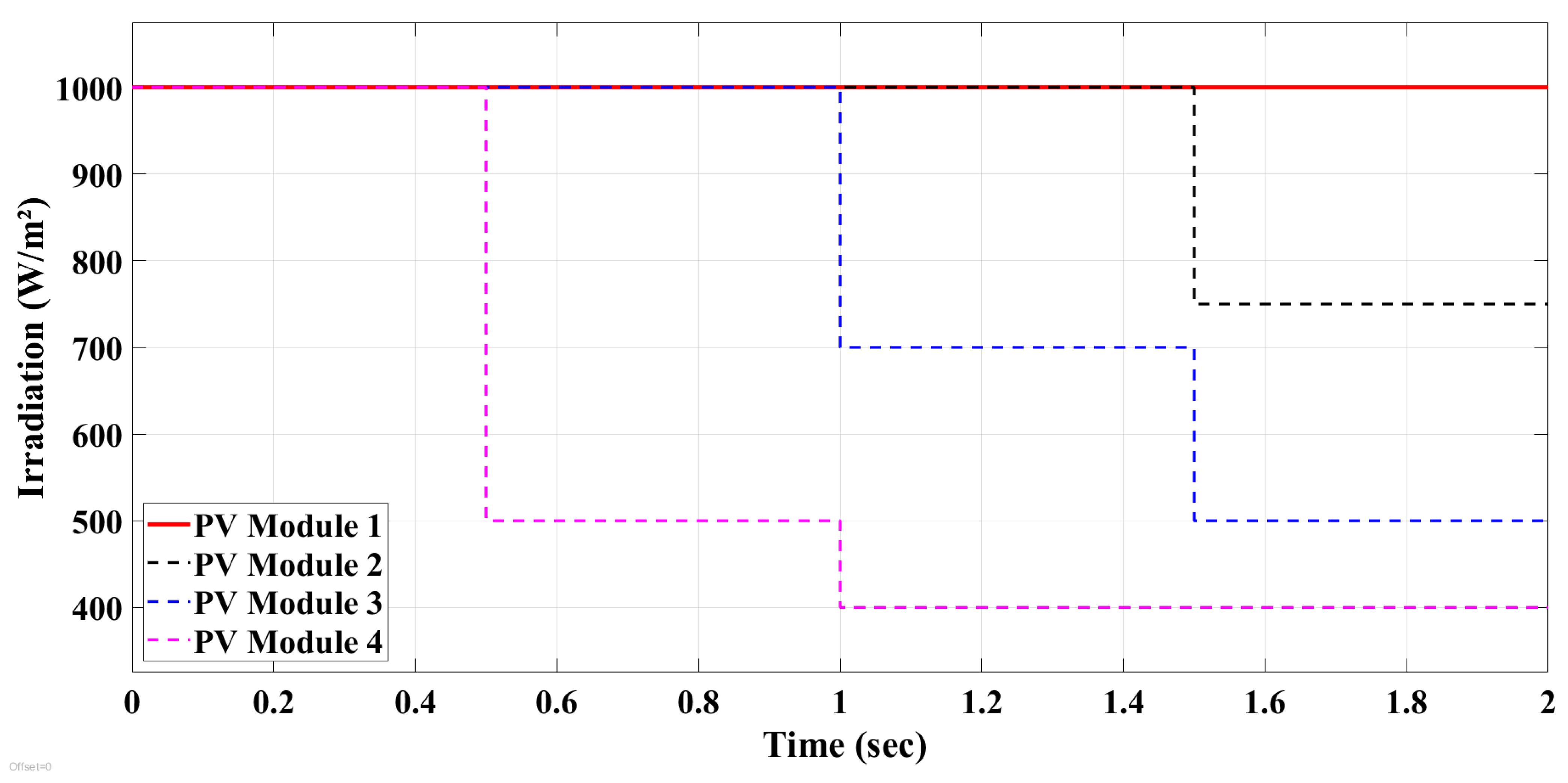
4.1. Simulation Study under Partial Shading Conditions

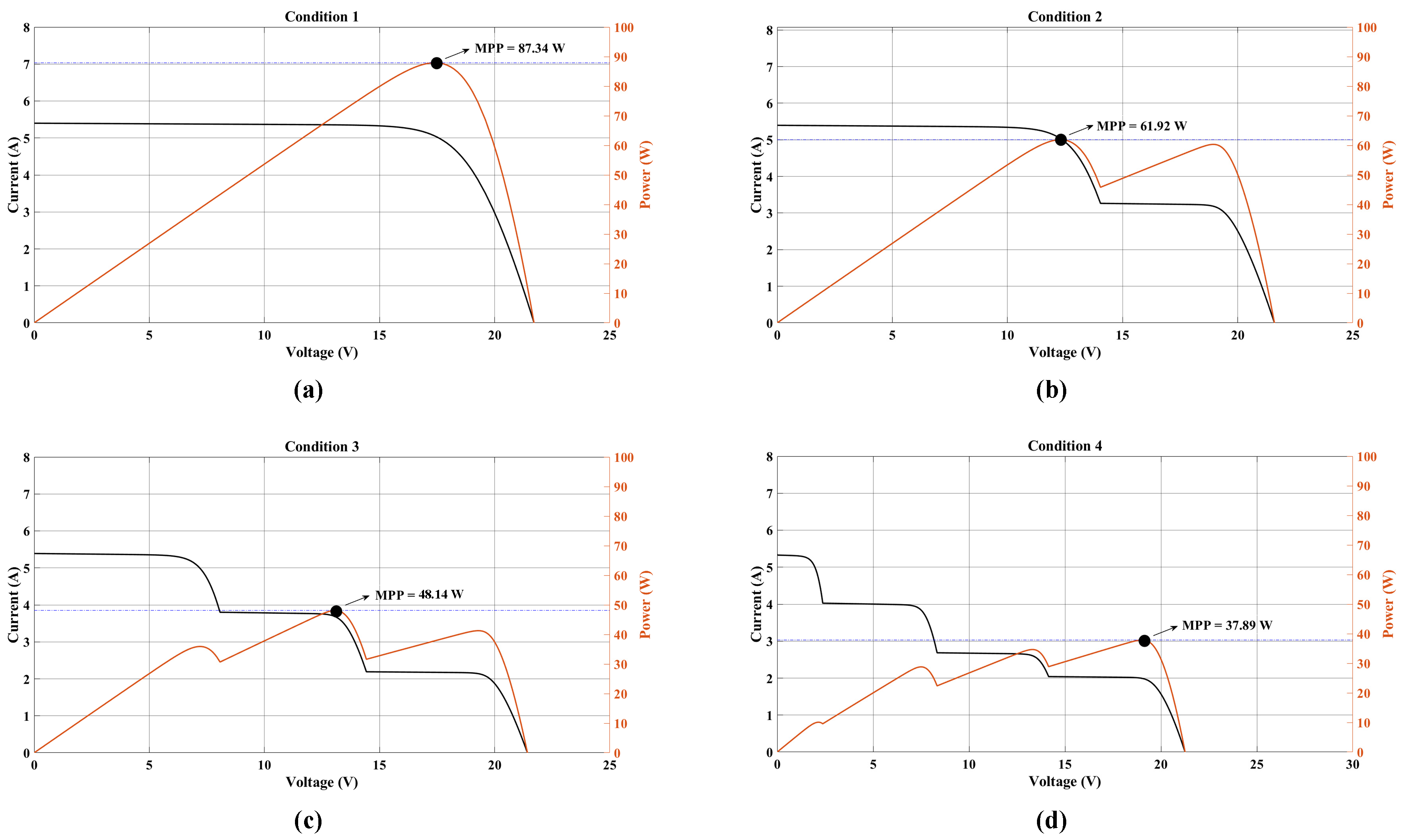
To evaluate the tracking capabilities of the newly developed DO-based MPP tracker, four distinct partial shading scenarios have been employed. These patterns, depicted in Figure 8, are listed below.

(1)

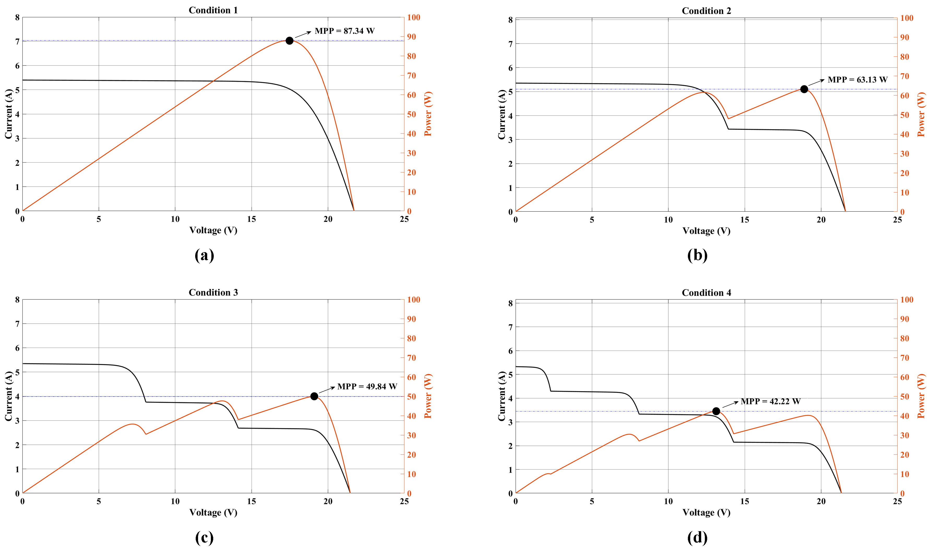
Pattern 1: In the first pattern, the simulation represents a scenario without any shading. In this configuration, all PV panels (G₁, G₂, G₃, G₄) receive an equal irradiation level of 1000 W/m², resulting in the generation of equal currents. As a result, the P-V curve displays a single peak with the maximum power, referred to as GMPP, as shown in Figure 8a.

(2)

Pattern 2: In this pattern, the simulation represents a light shade condition. In this configuration, modules G₁, G₂, and G₃ receive an irradiance of 1000 W/m², while module G₄ receives only 500 W/m² due to partial shading. Consequently, the current caused by the PV string and the shaded module are equal. However, the maximum current due to the unshaded PV panels can be bypassed through the bypass diodes across each panel. This disparity in currents results in the generation of two distinct peaks in the P-V curves, as illustrated in Figure 8b.

(3)

Pattern 3: In this pattern, the simulation depicts a scenario where modules G₁ and G₂ obtain an irradiance of 1000 W/m², while modules G₃ and G₄ receive 700 W/m² and 400 W/m², respectively, due to partial shading. Consequently, the current produced by the PV string aligns with that of the shaded modules (G₃ and G₄). This results in the generation of three distinct peaks in the P-V curves, owing to the variation in currents, as illustrated in Figure 8c.

(4)

Pattern 4: This pattern represents a strong shade condition, where PV modules G₁, G₂, G₃, and G₄ obtain irradiance levels of 1000 W/m², 750 W/m², 500 W/m², and 400 W/m², respectively. Each module experiences a different degree of shading, leading to the development of distinct currents. Consequently, the P-V curves exhibit multiple peaks, as depicted in Figure 8d. Among these peaks, only one corresponds to the GMPP, while the others are identified as LMPPs.

The average convergence curves for tracked PV power, current, voltage, and duty cycle are depicted in Figure 9, Figure 10 and Figure 11 for the DO, CS, and PSO algorithms, respectively. These curves serve as a basis for evaluating the reliability, efficiency, and accuracy of the proposed algorithm in tracking the GMPP under the four different situations.

The performance of the DO algorithm is examined and compared to the CS and PSO algorithms in the following discussions. The evaluation consists of testing the algorithms with various shade patterns and measuring their performance in terms of tracked power levels, tracking time, and effectiveness in reaching the GMPP.

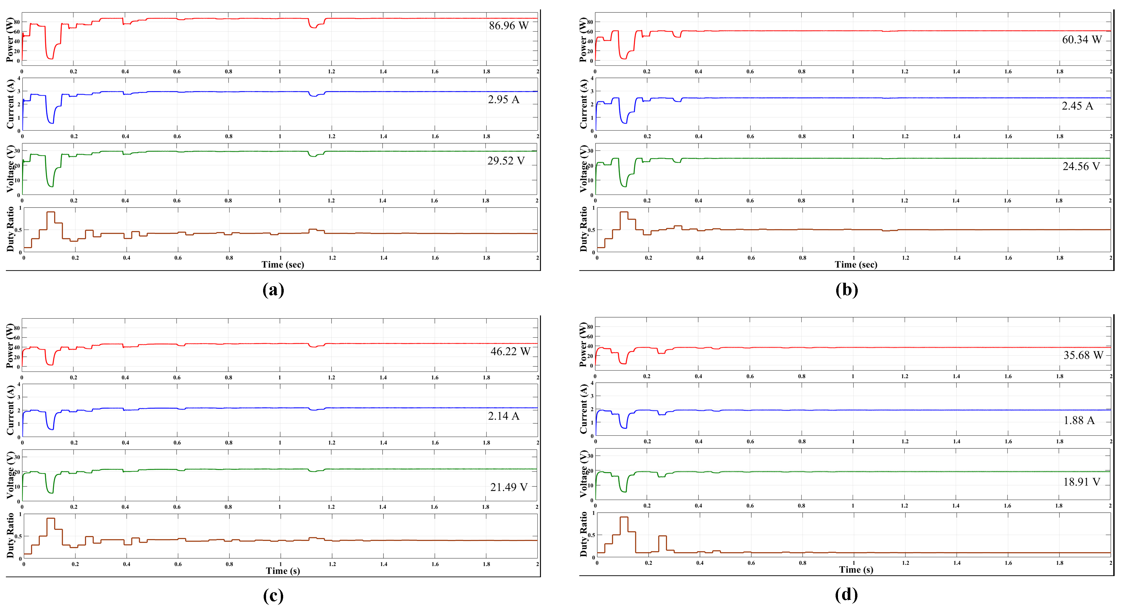
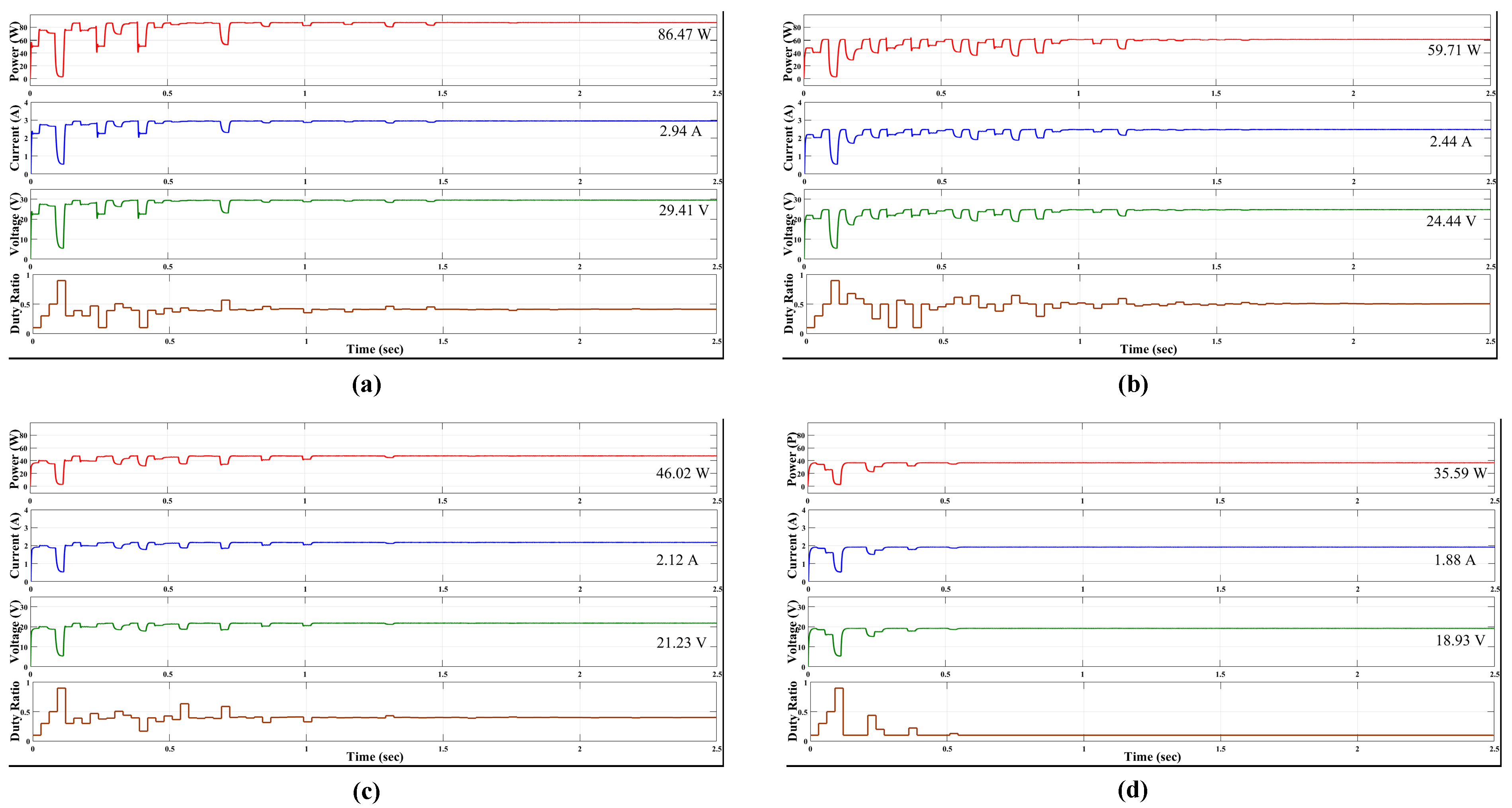
4.1.1. Shading Condition 1

The PV modules in this experiment receive a uniform 1000 W/m². Results show that DO exhibits significantly lower convergence time and negligible size fluctuations compared to PSO and CS. Furthermore, as shown in Figure 9a, DO effectively tracks the MPP of 87.26 W, with a current of 2.94 A at MPP and voltage of 29.59 V at MPP, achieving a tracking efficiency of 99.90% with a measured convergence time of 0.25 s. On the other hand (Figure 10a), CS can track the MPP effectively and has a settling time of only 1.17 s, while DO displays a considerably faster settling time. It settles at a lower value of 86.96 W, with a current of 2.95 A at MPP and voltage of 29.52 V, achieving an efficiency of 99.56% (Figure 11a). PSO successfully tracks the MPP of 86.47 W, with a current of 2.94 A at MPP and voltage of 29.41 V, owing to its exploration and exploitation capabilities. However, it takes longer to settle than DO and CS, at 1.48 s. Despite settling at the MPP, the elevated steady-state oscillations in PSO lead to power losses, reducing its efficiency to 99.00%. In comparison to CS and PSO, DO shows a 492.00% and 368.00% improvement in settling time, respectively. It is worth noting that DO outperforms under full insolation conditions, but metaheuristic algorithms should also be suitable for partial shading scenarios.

4.1.2. Shading Condition 2

Under the second condition, the four modules of PV array experience varying insolation values of 1000, 1000, 1000, and 500 W/m², respectively. As seen in Figure 9b, DO effectively tracks the MPP of 61.71 W with a current of 2.48 A at MPP and voltage of 24.84 V at MPP in a settling time of 0.25 s, achieving an efficiency of almost 99.66% under the PS scenario. As seen in Figure 10b, CS achieves a slightly lesser tracking time of 0.34 s, settling at a lower MPP value of 60.34 W with a current of 2.45 A at MPP and voltage of 24.56 V at MPP and a lower efficiency of 97.44%. from Figure 11b PSO, on the other hand, tracks the MPP of 59.71 W with a current of 2.44 A at MPP and voltage of 24.44 V at MPP and an efficiency of 96.43%, which is lower than both DTBO and CS. Additionally, the settling time of PSO is longer at 1.38 s. When compared to CS and PSO, DO display significant improvement in settling time, with 36.00% and 452% advancement, respectively. These results suggest that DO has many advantages over competing algorithms specifically greater efficiency and shows a significant improvement in convergence rate.

4.1.3. Shading Condition 3

In condition 3, two panels receive full irradiance of 1000 W/m², and the remaining two panels receive 700 and 400 W/m², respectively (Figure 9c). DO achieves the MPP of (Figure 10c), CS takes longer to track the MPP, with a tracking time of 1.17 s, and settles at a lower value of 46.22 W with a current of 2.14 A at MPP and voltage of 21.49 V at MPP, resulting in an efficiency of 96.01%. As seen in Figure 11c, PSO also successfully tracks the MPP at 46.02 W with a current of 2.12 A at MPP and voltage of 21.23 V at MPP, but with a lower efficiency of 95.59% compared to DO. In this case, both CS and PSO exhibit lower efficiencies than DO. Moreover, the tracking time of PSO is longer than both DO and CS at 1.32 s. However, DO experiences fewer fluctuations during the search for the MPP than CS and PSO, leading to a significant reduction in power losses. DO also demonstrates a substantial improvement in settling time compared to CS and PSO, with percentages of 368% and 428%, respectively. These findings suggest that DO is more effective than competing algorithms and shows a significant improvement in convergence speed.

4.1.4. Shading Condition 4

This is a condition of strong PS, where the insolation varies across different panels with values of 1000, 750, 500, and W/m². In this setting (Figure 9d), the DO algorithm performs exceptionally well by accurately tracking the maximum power point (MPP) within just 0.10 s, achieving an impressive efficiency of nearly 97.25%. The DO algorithm also achieves an MPP of 36.85 W with a current of 1.91 A at MPP and a voltage of 19.20 V at MPP. On the other hand (Figure 10d), the CS algorithm exhibits a significantly slower tracking time of 0.48 s and settles at a lower value of 35.68 W with a current of 1.88 A at MPP and voltage of 18.91 V at MPP, resulting in an efficiency of 94.16%. Similarly, (Figure 11d), the PSO algorithm also tracks the MPP, but takes slightly longer than CS with a settling time of 0.54 s, achieving an efficiency of 93.92% and obtaining the MPP of 35.59 W with a current of 1.88 A at MPP and voltage of 18.93 V at MPP. The settling time of the DO algorithm improves by 380% and 440% compared to CS and PSO, respectively. Furthermore, both CS and PSO algorithms exhibit poor performance, as their convergence to the MPP occurs at a significantly slower rate, resulting in higher overall power losses. In conclusion, the DO algorithm outperforms the CS and PSO algorithms in terms of settling time and efficiency in a strong PS situation.

Table 4. Quantitative comparison of DO with CS and PSO.

Shading Condition	Insolation (W/m2)				Method	Imp (A)	Vmp (V)	Pmp (W)	Rated Power (W)	Eff. (%)	Settling Time (s)
	G1	G2	G3	G4
1	1000	1000	1000	1000	DO	2.94	29.59	87.26	87.34	99.90	0.25
					CS	2.95	29.52	86.96		99.56	1.17
					PSO	2.94	29.41	86.47		99.00	1.48
2	1000	1000	1000	500	DO	2.48	24.84	61.71	61.92	99.66	0.25
					CS	2.45	24.56	60.34		97.44	0.34
					PSO	2.44	24.44	59.71		96.43	1.38
3	1000	1000	700	400	DO	2.18	21.84	47.68	48.14	99.04	0.25
					CS	2.14	21.49	46.22		96.01	1.17
					PSO	2.12	21.23	46.02		95.59	1.32
4	1000	750	500	400	DO	1.91	19.20	36.85	37.89	97.25	0.10
					CS	1.88	18.91	35.68		94.16	0.48
					PSO	1.88	18.93	35.59		93.92	0.54

displays all the above simulation results and outcomes for different partial shading conditions: different insolation conditions corresponding to different conditions, current at maximum power (I_mp), voltage at maximum power (V_mp), maximum power (P_mp), rated power, efficiency, and settling time.

4.2. Simulation Study under Varying Irradiation

In this subsection, the performance of a DO-based MPPT technique is evaluated based on its ability to monitor and retrack the global MPP in the presence of fluctuating irradiance. A sequence of solar irradiation steps is applied to a PV array to simulate the effect of a cloud moving across the top of a PV array. The step changes occur at intervals of 0.5 s, as shown in Figure 12. The temperature remains constant at 25 °C throughout the test. The optimization results for MPPT under step change irradiations are presented in Figure 13.

The PV power plot in Figure 13 demonstrates that the DO algorithm tracks the MPP at 87.26 W under standard test conditions (STC) in the first interval, with an output current and voltage of 2.94 A and 29.59 V, respectively. The DO achieves an efficiency of 99.90% under STC and settles in 0.25 s. Under uniform irradiation conditions, the DO-based MPPT controller performs well with low computational power and does not produce any undesired oscillations around the global MPP. At 0.5 s, the irradiance pattern suddenly changes to 1000 W/m², 1000 W/m², 1000 W/m², and 500 W/m², respectively, in the four PV panels. During the second condition, which is a light shading scenario, the DO tracks the MPP at 61.71 W with an output current and voltage of 2.48 A and 24.84 V, respectively. The DO achieves an efficiency of 99.66% under this condition and settles at the same time as in the previous condition, i.e., 0.25 s. After 1 s, the irradiances on the four PV panels are changed to 1000 W/m², 1000 W/m², 700 W/m², and 400 W/m², respectively, in the third condition, which is a partial shading scenario. The DO tracks the MPP at 47.68 W with an output current and voltage of 2.18 A and 21.84 V, respectively. The DO achieves an efficiency of 99.04% under this condition and settles in 0.25 s. Finally, after 1.5 s, the irradiances on the four PV panels are changed to 1000 W/m², 750 W/m², 500 W/m², and 400 W/m², respectively, in the fourth condition, which is a strong and complex partial shading scenario. The DO tracks the MPP at 36.85 W with an output current and voltage of 1.91 A and 19.20 V, respectively. The DO achieves an efficiency of 97.25% under this condition, and its settling time is less than the previous conditions at 0.1 s. Furthermore, when solar irradiation suddenly changes, the DO algorithm produces output power, voltage, and current that do not exhibit any oscillations. This indicates that the DO-based MPPT controller has an inherent ability to adapt to different weather conditions and significantly improve the probability of obtaining a high-quality optimum power point through global and local exploration.

5. Hardware-in-the-Loop (HIL) Implementation

In this section, the DO algorithm is tested using the Typhoon Hardware-In-Loop (HIL) 402 emulator, as demonstrated in Figure 13. The MPPT algorithm is built into the advanced C function block of the Typhoon HIL model, which operates in a manner analogous to that of a microcontroller. In particular, the DO-based MPPT technique is contrasted to the CS and PSO algorithms in terms of their convergence time to the GMPP, efficiency, and the number and amplitude of fluctuations after initialization. Table 1 and Table 2 detail the dimensions and ratings of the PV module and DC-DC boost converter utilized in the experiment. The Typhoon-HIL emulation setup is shown in Figure 14. The Typhoon-HIL analysis confirms the real-time implementation of the DO algorithm, providing assurance that the method is effective and applicable in real-world scenarios with varying solar radiation intensity.

5.1. Static Shading Conditions

To assess the tracking capabilities of the newly developed DO-based MPP tracker, four distinct partial shading scenarios have been utilized, as depicted in Figure 15 and described below.

(1)

In scenario 1, there is no shading, and all photovoltaic (PV) panels—G₁, G₂, G₃, and G₄—receive an equal irradiation level of 1000 W/m². This uniform irradiation leads to the generation of equal currents. The corresponding P-V curve demonstrates a solitary peak, referred to as the GMPP, as shown in Figure 15a.

(2)

In scenario 2, a light shading condition is present, where only the G₄ module receives an irradiance of 600 W/m², while the remaining modules—G₁, G₂, and G₃—receive an irradiance of 1000 W/m². The presence of bypass diodes enables the bypassing of the maximum current generated by the unshaded PV panels. As a result, the P-V curves have two separate peaks. This behavior is depicted in Figure 15b.

(3)

In the third scenario, the PV modules experience different levels of irradiance: G₁ and G₂ receive 1000 W/m², G₃ receives 700 W/m², and G₄ receives 500 W/m². Consequently, the shaded modules G₃ and G₄ generate lower currents than the unshaded modules. This difference in currents, assisted by the bypass diode, causes the P-V curves to exhibit three separate peaks. Figure 15c visually represents these peaks.

(4)

Scenario 4 is characterized by a significant shading effect, where each PV panel experiences a different level of shading. This circumstance causes several peaks to appear on the P-V curves. Specifically, the G₁, G₂, G₃, and G₄ modules receive irradiance levels of 1000 W/m², 700 W/m², 600 W/m², and 400 W/m², respectively. In this scenario, only one peak corresponds to the GMPP, while the other peaks are regarded as LMPPs. The behavior of the P-V curve under this scenario is illustrated in Figure 15d.

Figure 16, Figure 17 and Figure 18 provide the mean convergence curves for tracked PV parameters, such as power, current, voltage, and duty cycle, to evaluate the dependability, efficiency, and precision, of the proposed algorithm in monitoring the GMPP under different shading situations. These figures showcase the performance of the DO, CS, and PSO algorithms. In the subsequent analysis, the DO algorithm is assessed under various shading conditions and compared to the CS and PSO techniques based on their ability to track the GMPP, tracking time, and power tracking accuracy.

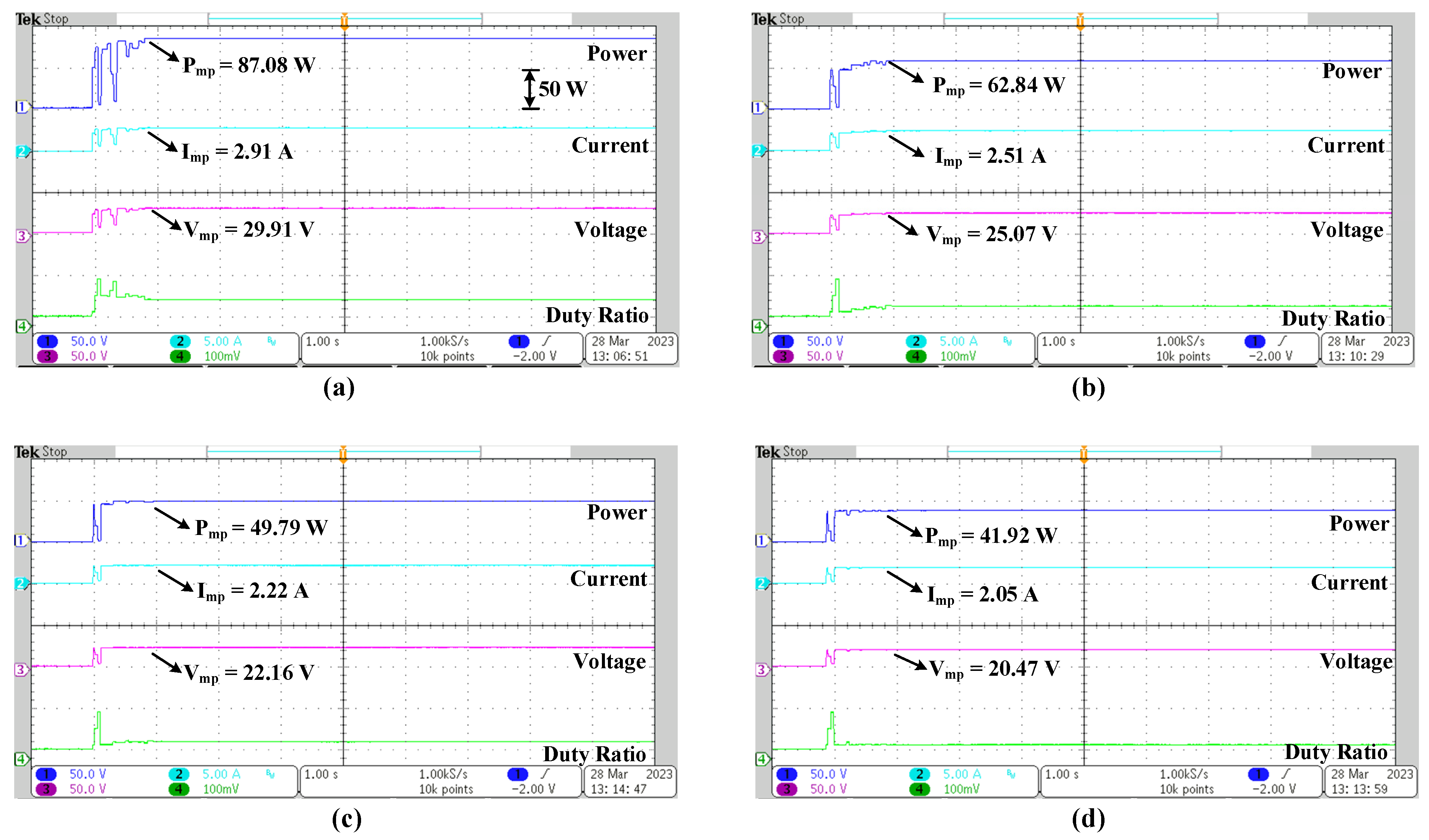
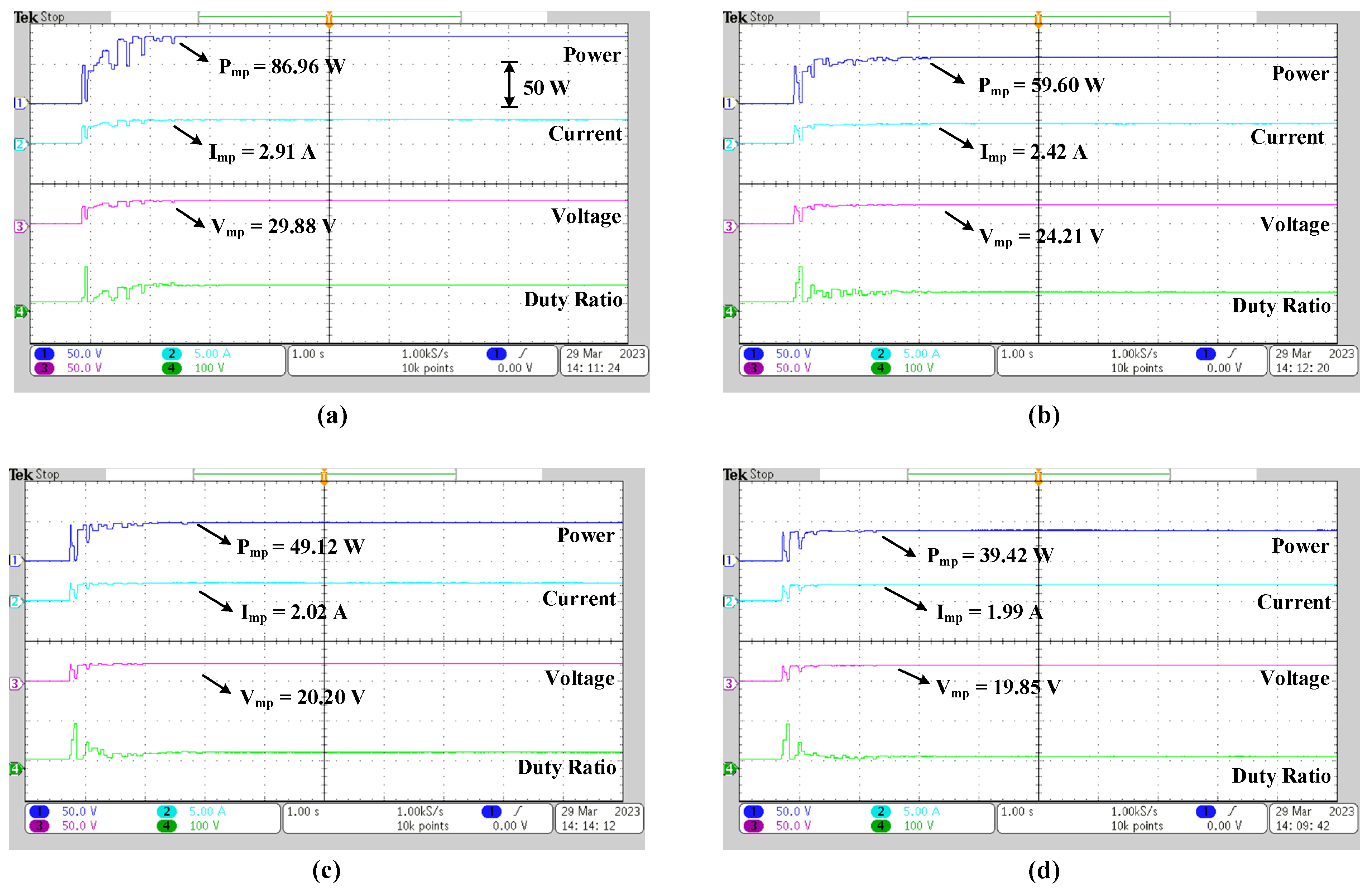
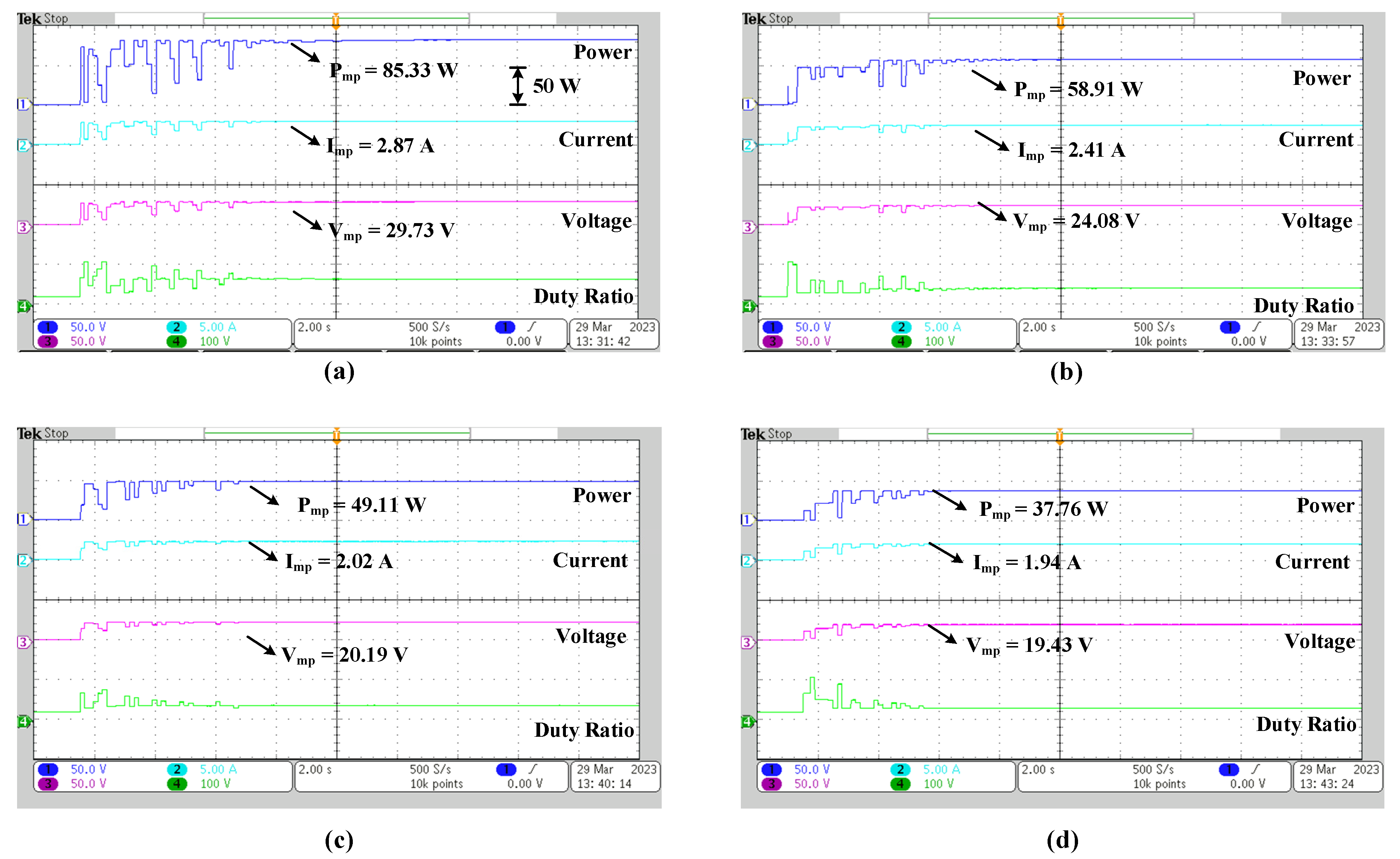
5.1.1. Shading Condition 1

Based on the comparison plots provided in Figure 16a, Figure 17a and Figure 18a, the three algorithms (DO, CS, and PSO) were compared for a four-module PV array under full irradiance conditions of 1000 W/m² in terms of tracking time and efficiency. The shading condition, the method used, and important parameters such as I_mp (current at MPP), V_mp (voltage at MPP), P_mp (power at MPP), rated power, efficiency, and tracking time were also taken into account. DO effectively tracks the MPP of 87.08 W, with a current of 2.91 A at MPP and voltage of 29.91 V at MPP, whereas PSO tracks the MPP of 85.33 W, with a current of 2.87 A at MPP and voltage of 29.73 V at MPP, and CS tracks the MPP of 86.96 W, with a current of 2.91 A at MPP and voltage of 29.88 V at MPP, In terms of tracking time, the PSO algorithm has the longest time of 6.8 s, followed by the DO algorithm with a time of 0.8 s, while the CS algorithm has the shortest time of 1.6 s. Regarding efficiency, the DO algorithm has the highest efficiency of 99.02%, followed by the CS algorithm with an efficiency of 98.88%, and the PSO algorithm with the lowest efficiency of 97.03%. In comparison to CS and PSO, DO shows a 100.00% and 750.00% improvement in settling time, respectively. Overall, the DO algorithm seems to be the most efficient of the three algorithms, despite having a longer tracking time than the CS algorithm. Meanwhile, the PSO algorithm has the lowest efficiency and longest tracking time, indicating that it may not be the best choice for this particular scenario.

5.1.2. Shading Condition 2

Figure 16b, Figure 17b and Figure 18b compare the tracking efficiency and tracking time of the three algorithms under irradiance conditions of 1000, 1000, 1000 and 600 W/m², respectively, on the four modules of the PV array. DO effectively tracks the MPP of 62.84 W, with a current of 2.51 A at MPP and voltage of 25.07 V at MPP, whereas PSO tracks the MPP of 58.91 W, with a current of 2.41 A at MPP and voltage of 24.08 V at MPP, and CS tracks the MPP of 59.60 W, with a current of 2.42 A at MPP and voltage of 24.21 V at MPP. Under these conditions, DO achieves the highest efficiency of 99.54%, with a tracking time of 0.8 s and a duty ratio of 0.51. CS achieves an efficiency of 94.40% with a tracking time of 2.4 s and the same duty ratio as DO. PSO has the lowest efficiency of the three, at 93.31%, with a tracking time of 5 s and the same duty ratio as the other two algorithms. In comparison to CS and PSO, DO shows a 200.00% and 525.00% improvement in settling time, respectively. Overall, DO appears to be the most efficient and fastest algorithm under these shading conditions, followed by CS and then PSO. Nevertheless, it should be acknowledged that the effectiveness of each algorithm may differ based on the specific shading conditions and other contextual factors within a particular application.

5.1.3. Shading Condition 3

The performances of three algorithms are compared based on tracking time and efficiency across four modules of a PV array, considering partial irradiances of 1000, 1000, 700, and 500 W/m². Figure 16c, Figure 17c and Figure 18c illustrate these comparisons. The DO achieved I_mp at 2.22 A, with V_mp at 22.16 V, and P_mp at 49.79 W. Its overall efficiency is calculated to be 99.89% with a tracking time of 1.0 s. CS resulted in slightly lower values, with I_mp at 2.02 A, V_mp at 20.20 V, and P_mp at 49.12 W. The efficiency of CS is found to be 98.55% with a tracking time of 2.0 s. PSO has similar I_mp values of 2.02 A, V_mp at 20.19 V, and P_mp at 49.11 W. Its efficiency is slightly lower than CS at 98.53%, and the tracking time is the longest at 4.8 s. In comparison to CS and PSO, DO demonstrated a 100.00% and 380.00% improvement in settling time, respectively. Overall, DO exhibited the best efficiency and tracking time, followed by PSO and CS.

5.1.4. Shading Condition 4

Based on the data from Figure 16d, Figure 17d and Figure 18d, the tracking time and efficiency of three algorithms were evaluated for a four-module photovoltaic array under complex partial shading conditions of 1000, 700, 600, and 400 W/m². DO achieved an I_mp value of 2.05 A, with V_mp at 20.47 V, and P_mp at 41.92 W. Its overall efficiency is found to be 99.28%, with a tracking time of 1.0 s. CS has a slightly lower I_mp value of 1.99 A, with V_mp at 19.85 V, and P_mp at 39.42 W. The overall efficiency of CS is significantly lower than DO at 93.36%, and it requires a longer tracking time of 2.6 s. PSO obtained the lowest I_mp value of 1.94 A, with V_mp at 19.43 V, and P_mp at 37.76 W. Its efficiency is the lowest among the three algorithms for this condition at 89.43%, and it has the longest tracking time of 4.0 s. Comparing the results, the DO outperformed both CS and PSO with a settling time improvement of 160.00% and 300.00%, respectively. In terms of efficiency and tracking time, the DO algorithm demonstrated the highest effectiveness, followed by CS and PSO algorithms.

The findings suggest that the DO algorithm is the most efficient and effective choice for MPPT in the complex partial shading conditions. It significantly outperforms CS and PSO in terms of both tracking time and efficiency, making it a promising solution for optimizing PV array performance under challenging environmental conditions.

The HIL implementation analysis and outcomes under various partial shading conditions are presented in

Table 5. Quantitative comparison of DO with CS and PSO.

Shading Condition	Insolation (W/m2)				Method	Imp (A)	Vmp (V)	Pmp (W)	Rated Power (W)	Eff. (%)	Settling Time (s)
	G1	G2	G3	G4
1	1000	1000	1000	1000	DO	2.91	29.91	87.08	87.34	99.70	0.8
					CS	2.91	29.88	86.96		99.56	1.6
					PSO	2.87	29.73	85.33		97.69	6.8
2	1000	1000	1000	600	DO	2.51	25.07	62.84	63.13	99.54	0.8
					CS	2.42	24.21	59.60		94.40	2.4
					PSO	2.41	24.08	58.91		93.31	5.0
3	1000	1000	700	500	DO	2.22	22.16	49.79	49.84	99.89	1.0
					CS	2.02	20.20	49.12		98.55	2.0
					PSO	2.02	20.19	49.11		98.53	4.8
4	1000	700	600	400	DO	2.05	20.47	41.92	42.22	99.28	1.0
					CS	1.99	19.85	39.42		93.36	2.6
					PSO	1.94	19.43	37.76		89.43	4.0

. The table shows the corresponding I_mp, V_mp, P_mp, rated power, efficiency, and settling time for the different irradiance conditions.

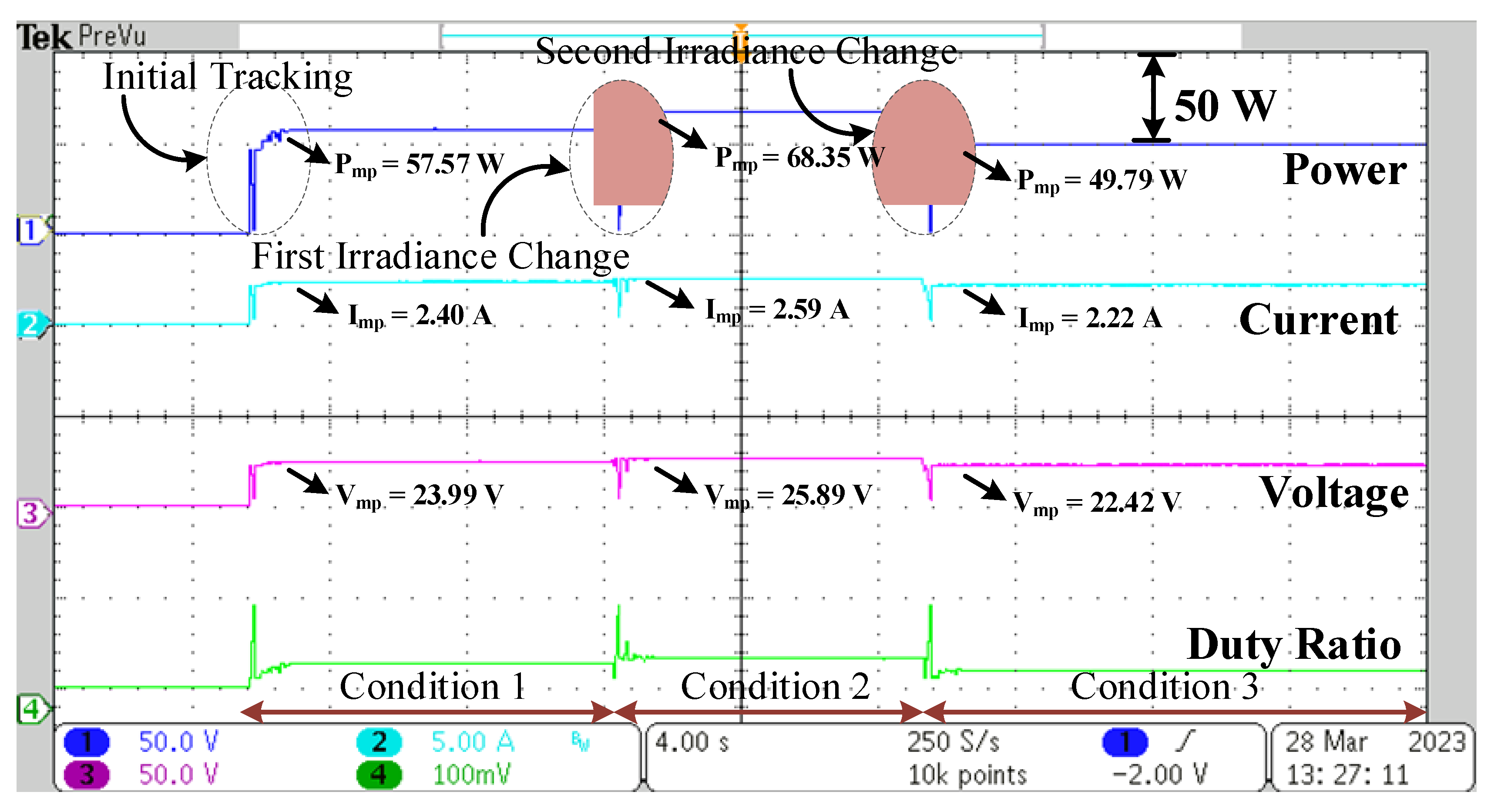
5.2. Dynamic Changes in Shading Pattern

This subsection showcases the practical adaptability of the proposed DO algorithm by simulating changes in shading patterns over time. These changes may result from various factors such as cloud movement and sun position. The PV modules are subjected to different shading patterns, as listed in

Table 6. Summary of results obtained with dynamic changes in irradiance.

Irradiance Condition	Insolation (W/m2)				Imp (A)	Vmp (V)	Pmp (W)	Rated Power (W)	Eff. (%)	Settling Time (s)
	G1	G2	G3	G4
1	1000	1000	700	600	2.40	23.99	57.57	87.34	98.22	1.0
2	1000	1000	700	1000	2.59	25.89	68.35	63.13	98.84	1.6
3	1000	500	700	1000	2.22	22.42	49.79	49.84	99.89	1.6

, and real-time results are generated.

Figure 19 illustrates the performance curves of the DO algorithm under different shading situations. The graph displays the effect of the dynamic changes in irradiances on the PV array, which is similar to when a cloud initially results in partial shading and subsequently moves away over time, exposing or covering the surface of the PV array. Under condition 1, the DO algorithm achieves an I_mp of 2.40 A and V_mp of 23.99 V, with a P_mp of 57.57 W and an efficiency of 98.22%, with a tracking time of 1.0 s. In condition 2, the DO algorithm attains a maximum efficiency of 98.84%, tracking the P_mp with a tracking time of 1.6 s at 68.35 W, and an I_mp value of 2.59 A. Lastly, under condition 3, the DO algorithm achieves a maximum efficiency of 99.89%, with an I_mp value of 2.22 A and a V_mp of 22.42 V, with a tracking time of 1.6 s. In addition, the DO algorithm is observed to produce stable output power, voltage, and current when the solar irradiation suddenly changes. This suggests that the DO-based MPPT controller can effectively adapt to varying weather conditions and increase the likelihood of achieving an optimal power point through both global and local exploration.

6. Discussion

The novelty of using the DO algorithm for MPPT compared to other algorithms lies in its unique modeling of dandelion seed flight dynamics and trajectory patterns, which enables it to achieve a harmonious blend of exploration and exploitation. These distinctive features enhance the precision and efficacy of locating the GMPP in PV systems. The key elements that set DO apart from other algorithms are as follows.

• Three-Stage Process: DO models the dandelion seed flight dynamics as a three-stage process: rise, descent, and landing. Each stage is designed to serve a specific purpose in the optimization process, making the algorithm more effective in capturing the GMPP.
• Incorporation of Random Trajectories: In the rising stage, DO incorporates random trajectories. By doing so, the algorithm can easily adjust to different weather conditions, which is particularly beneficial in real-world PV systems that experience varying environmental factors. This adaptability allows DO to efficiently explore the search space and avoid becoming trapped in local optima.
• Utilization of Brownian Motion and Levy Flight: In the descending stage, DO employs Brownian motion trajectory, which adds a level of randomness to the movement, helping to further explore the search space. Additionally, in the landing stage, DO uses a linear increasing function with Levy flight. Levy flight is known for its ability to perform long-range jumps, facilitating a more thorough exploration of the search space.
• Harmonious Exploration and Exploitation: The trajectory patterns exhibited by DO, combining random trajectories, Brownian motion, and Levy flight, enable the algorithm to achieve a harmonious balance between exploration (discovering new areas in the search space) and exploitation (focusing on promising regions). This balance is essential in effectively locating the GMPP, as it prevents premature convergence and ensures that the algorithm explores potential optimal solutions.
• Precision in GMPP Localization: By incorporating these trajectory patterns and balancing exploration and exploitation, DO enhances the precision in locating the GMPP. The algorithm can quickly and accurately track the optimal power output, leading to improved MPPT performance and higher energy harvesting efficiency in PV systems.

In conclusion, the novelty of using the DO algorithm for MPPT lies in its unique modeling of dandelion seed flight dynamics, including the three-stage process and the use of random trajectories, Brownian motion, and Levy flight. The elements enable DO to strike a harmonious balance between exploration and exploitation, resulting in improved precision and effectiveness in locating the GMPP across diverse weather conditions and dynamic environments. Notably, the proposed DO approach proves to be particularly valid for addressing shading caused by pollution, enclosing structures, and flying objects. This innovation makes DO a promising and innovative option for implementing MPPT in photovoltaic systems.

7. Conclusions

This research presents a detailed controller for maximum power point tracking (MPPT) in photovoltaic (PV) arrays, incorporating the novel dandelion optimizer (DO) method implemented using MATLAB/Simulink software. The study compares the effectiveness of the DO algorithm with two other popular algorithms—cuckoo search (CS) and particle swarm optimization (PSO)—in terms of MPPT accuracy, tracking time, and efficiency.

The findings reveal that the DO algorithm outperforms both CS and PSO. On average, the DO algorithm achieves a tracking time of 0.2125 s and an efficiency of 98.96%. In comparison, CS takes 0.79 s with an efficiency of 96.79%, and PSO takes 1.18 s with an efficiency of 96.235%. Moreover, real-time simulation analysis using a hardware-in-the-loop (HIL) 402 emulator verifies the advantages of the DO algorithm. On average, DO achieves a tracking time of 0.9 s, while CS and PSO take 2.15 s and 5.15 s, respectively. Additionally, DO exhibits the highest efficiency at 99.60%, surpassing CS (96.46%) and PSO (94.74%).

The obtained results demonstrate that the proposed DO-based MPPT approach is reliable, efficient, accurate, and fast, even in challenging scenarios involving partial shading. This research showcases the capability of the DO algorithm to achieve its intended objectives effectively. Further research could explore the application of the DO algorithm in MPPT controllers for other renewable energy sources such as wind and hydro, as well as its performance in grid-connected PV systems. These investigations would contribute to advancing the understanding and application of DO in various renewable energy domains.

References

1. Belhachat, F.; Larbes, C. Comprehensive review on global maximum power point tracking techniques for PV systems subjected to partial shading conditions. Sol. Energy 2019, 183, 476–500. [Google Scholar] [CrossRef]
2. Yang, B.; Zhu, T.; Wang, J.; Shu, H.; Yu, T.; Zhang, X.; Yao, W.; Sun, L. Comprehensive overview of maximum power point tracking algorithms of PV systems under partial shading condition. J. Clean. Prod. 2020, 268, 121983. [Google Scholar] [CrossRef]
3. Yang, B.; Zhong, L.; Zhang, X.; Shu, H.; Yu, T.; Li, H.; Jiang, L.; Sun, L. Novel bio-inspired memetic salp swarm algorithm and application to MPPT for PV systems considering partial shading condition. J. Clean. Prod. 2019, 215, 1203–1222. [Google Scholar] [CrossRef]
4. Rehman, H.; Sajid, I.; Sarwar, A.; Tariq, M.; Bakhsh, F.I.; Ahmad, S.; Mahmoud, H.A.; Aziz, A. Driving training-based optimization (DTBO) for global maximum power point tracking for a photovoltaic system under partial shading condition. IET Renew. Power Gener. 2023, 17, 2542–2562. [Google Scholar] [CrossRef]
5. Zafar, M.H.; Khan, N.M.; Mirza, A.F.; Mansoor, M. Bio-inspired optimization algorithms based maximum power point tracking technique for photovoltaic systems under partial shading and complex partial shading conditions. J. Clean. Prod. 2021, 309, 127279. [Google Scholar] [CrossRef]
6. Sajid, I.; Sarwar, A.; Tariq, M.; Bakhsh, F.I.; Hussan, R.; Ahmad, S.; Mohamed, A.S.N.; Ahmad, A. Runge Kutta optimization-based selective harmonic elimination in an H-bridge multilevel inverter. IET Power Electron. 2023. [Google Scholar] [CrossRef]
7. Sajid, I.; Iqbal, D.; Alam, M.S.; Rafat, Y.; Al Ammar, E.; Alrajhi, H. Feasibility Analysis of Open Vehicle Grid Integration Platform (OVGIP) for Indian Scenario. In Proceedings of the 2022 2nd International Conference on Advances in Electrical, Computing, Communication and Sustainable Technologies, ICAECT, Bhilai, India, 21–22 April 2022. [Google Scholar] [CrossRef]
8. Seyedmahmoudian, M.; Soon, T.K.; Horan, B.; Ghandhari, A.; Mekhilef, S.; Stojcevski, A. New ARMO-based MPPT Technique to Minimize Tracking Time and Fluctuation at Output of PV Systems under Rapidly Changing Shading Conditions. IEEE Trans. Ind. Inform. 2019. [Google Scholar] [CrossRef]
9. Awan, M.M.A.; Asghar, A.B.; Javed, M.Y.; Conka, Z. Ordering Technique for the Maximum Power Point Tracking of an Islanded Solar Photovoltaic System. Sustainability 2023, 15, 3332. [Google Scholar] [CrossRef]
10. Yousri, D.; Babu, T.S.; Allam, D.; Ramachandaramurthy, V.K.; Etiba, M.B. A Novel Chaotic Flower Pollination Algorithm for Global Maximum Power Point Tracking for Photovoltaic System Under Partial Shading Conditions. IEEE Access 2019, 7, 121432–121445. [Google Scholar] [CrossRef]
11. Pervez, I.; Pervez, A.; Tariq, M.; Sarwar, A.; Chakrabortty, R.K.; Ryan, M.J. Rapid and Robust Adaptive Jaya (Ajaya) Based Maximum Power Point Tracking of a PV-Based Generation System. IEEE Access 2021, 9, 48679–48703. [Google Scholar] [CrossRef]
12. Abdel-Salam, M.; El-Mohandes, M.-T.; Goda, M. An improved perturb-and-observe based MPPT method for PV systems under varying irradiation levels. Sol. Energy 2018, 171, 547–561. [Google Scholar] [CrossRef]
13. Fatemi, S.M.; Shadlu, M.S.; Talebkhah, A. Comparison of Three-Point P&O and Hill Climbing Methods for Maximum Power Point Tracking in PV Systems. In Proceedings of the 2019 10th International Power Electronics, Drive Systems and Technologies Conference (PEDSTC), Shiraz, Iran, 12–14 February 2019; pp. 764–768. [Google Scholar] [CrossRef]
14. Safari, A.; Mekhilef, S. Simulation and Hardware Implementation of Incremental Conductance MPPT With Direct Control Method Using Cuk Converter. IEEE Trans. Ind. Electron. 2010, 58, 1154–1161. [Google Scholar] [CrossRef]
15. Sher, H.A.; Murtaza, A.F.; Noman, A.; Addoweesh, K.E.; Al-Haddad, K.; Chiaberge, M. A New Sensorless Hybrid MPPT Algorithm Based on Fractional Short-Circuit Current Measurement and P&O MPPT. IEEE Trans. Sustain. Energy 2015, 6, 1426–1434. [Google Scholar] [CrossRef]
16. Baimel, D.; Tapuchi, S.; Levron, Y.; Belikov, J. Improved Fractional Open Circuit Voltage MPPT Methods for PV Systems. Electronics 2019, 8, 321. [Google Scholar] [CrossRef]
17. Debnath, A.; Olowu, T.O.; Parvez, I.; Dastgir, M.G.; Sarwat, A. A Novel Module Independent Straight Line-Based Fast Maximum Power Point Tracking Algorithm for Photovoltaic Systems. Energies 2020, 13, 3233. [Google Scholar] [CrossRef]
18. Algarín, C.R.; Giraldo, J.T.; Álvarez, O.R. Fuzzy Logic Based MPPT Controller for a PV System. Energies 2017, 10, 2036. [Google Scholar] [CrossRef]
19. Jyothy, L.P.; Sindhu, M.R. An Artificial Neural Network based MPPT Algorithm for Solar PV System. In Proceedings of the 2018 4th International Conference on Electrical Energy Systems (ICEES), Chennai, India, 7–9 February 2018; pp. 375–380. [Google Scholar] [CrossRef]
20. Li, X.; Wen, H.; Hu, Y.; Jiang, L. A novel beta parameter based fuzzy-logic controller for photovoltaic MPPT application. Renew. Energy 2019, 130, 416–427. [Google Scholar] [CrossRef]
21. Hai, T.; Zhou, J.; Muranaka, K. An efficient fuzzy-logic based MPPT controller for grid-connected PV systems by farmland fertility optimization algorithm. Optik 2022, 267, 169636. [Google Scholar] [CrossRef]
22. Hayder, W.; Ogliari, E.; Dolara, A.; Abid, A.; Ben Hamed, M.; Sbita, L. Improved PSO: A Comparative Study in MPPT Algorithm for PV System Control under Partial Shading Conditions. Energies 2020, 13, 2035. [Google Scholar] [CrossRef]
23. Alshareef, M.; Lin, Z.; Ma, M.; Cao, W. Accelerated Particle Swarm Optimization for Photovoltaic Maximum Power Point Tracking under Partial Shading Conditions. Energies 2019, 12, 623. [Google Scholar] [CrossRef]
24. Mosaad, M.I.; El-Raouf, M.O.A.; Al-Ahmar, M.A.; Banakher, F.A. Maximum Power Point Tracking of PV system Based Cuckoo Search Algorithm; review and comparison. Energy Procedia 2019, 162, 117–126. [Google Scholar] [CrossRef]
25. Cuong-Le, T.; Minh, H.-L.; Khatir, S.; Wahab, M.A.; Tran, M.T.; Mirjalili, S. A novel version of Cuckoo search algorithm for solving optimization problems. Expert Syst. Appl. 2021, 186, 115669. [Google Scholar] [CrossRef]
26. Gonzalez-Castano, C.; Restrepo, C.; Kouro, S.; Rodriguez, J. MPPT Algorithm Based on Artificial Bee Colony for PV System. IEEE Access 2021, 9, 43121–43133. [Google Scholar] [CrossRef]
27. Boutasseta, N.; Bouakkaz, M.S.; Fergani, N.; Attoui, I.; Bouraiou, A.; Neçaibia, A. Experimental Evaluation of Moth-Flame Optimization Based GMPPT Algorithm for Photovoltaic Systems Subject to Various Operating Conditions. Appl. Sol. Energy 2022, 58, 1–14. [Google Scholar] [CrossRef]
28. Guo, K.; Cui, L.; Mao, M.; Zhou, L.; Zhang, Q. An Improved Gray Wolf Optimizer MPPT Algorithm for PV System with BFBIC Converter Under Partial Shading. IEEE Access 2020, 8, 103476–103490. [Google Scholar] [CrossRef]
29. Mansoor, M.; Mirza, A.F.; Ling, Q.; Javed, M.Y. Novel Grass Hopper optimization based MPPT of PV systems for complex partial shading conditions. Sol. Energy 2020, 198, 499–518. [Google Scholar] [CrossRef]
30. Kaya, C.B.; Kaya, E.; Gökkuş, G. Training Neuro-Fuzzy by Using Meta-Heuristic Algorithms for MPPT. Comput. Syst. Sci. Eng. 2022, 45, 69–84. [Google Scholar] [CrossRef]
31. Zhao, S.; Zhang, T.; Ma, S.; Chen, M. Dandelion Optimizer: A nature-inspired metaheuristic algorithm for engineering applications. Eng. Appl. Artif. Intell. 2022, 114, 105075. [Google Scholar] [CrossRef]
32. Oliva, D.; Cuevas, E.; Pajares, G. Parameter identification of solar cells using artificial bee colony optimization. Energy 2014, 72, 93–102. [Google Scholar] [CrossRef]
33. Ghani, F.; Rosengarten, G.; Duke, M.; Carson, J. The numerical calculation of single-diode solar-cell modelling parameters. Renew. Energy 2014, 72, 105–112. [Google Scholar] [CrossRef]
34. Bastidas-Rodriguez, J.; Petrone, G.; Ramos-Paja, C.; Spagnuolo, G. A genetic algorithm for identifying the single diode model parameters of a photovoltaic panel. Math. Comput. Simul. 2017, 131, 38–54. [Google Scholar] [CrossRef]
Figure 1. Structure of standard PV cell with DC-DC boost converter and MPPT control. (G: irradiance (W/m2), Ipv: PV current (A), Vpv: PV Voltage (V), Cin: input-side capacitance (μF), L: inducatance (mH), D: diode, M: MOSFET, Cout: output-side capacitance (μF), RL: resistive load (Ω)).
Processes 11 02493 g001
Figure 2. PV cell model with single diode.
Processes 11 02493 g002
Figure 3. P-V and I-V characteristics at 1000 W/m2 of irradiance and varying temperatures.
Processes 11 02493 g003
Figure 4. P-V and I-V characteristics at an ambient temperature of 25 °C under varying solar irradiance.
Processes 11 02493 g004
Figure 5. P-V and I-V curves of series-connected PV modules under (a) nonuniform irradiance; (b) uniform irradiance.
Processes 11 02493 g005
Figure 6. Trajectories of dandelion seeds during the three stages of DO implementation: (a) rising stage; (b) descending stage; and (c) landing stage.
Processes 11 02493 g006
Figure 7. Flowchart of DO for MPPT control in PV system.
Processes 11 02493 g007
Figure 8. P-V and I-V plots were obtained for (a) condition 1, (b) condition 2, (c) condition 3, and (d) condition 4.
Processes 11 02493 g008
Figure 9. Plots of PV output power, current, voltage, and duty ratio produced for DO in (a) condition 1, (b) condition 2, (c) condition 3, and (d) condition 4.
Processes 11 02493 g009
Figure 10. Plots of PV output power, current, voltage, and duty ratio produced for CS in (a) condition 1, (b) condition 2, (c) condition 3, and (d) condition 4.
Processes 11 02493 g010
Figure 11. Plots of PV output power, current, voltage, and duty ratio produced for PSO in (a) condition 1, (b) condition 2, (c) condition 3, and (d) condition 4.
Processes 11 02493 g011
Figure 12. Step changes in solar irradiation of the four PV modules under different partial shading conditions.
Processes 11 02493 g012
Figure 13. The PV output power, current, voltage, and duty ratio plots obtained for DO as the irradiance pattern on the four PV panels is changed from condition 1 to condition 2, then to condition 3, and finally to condition 4 at intervals of 0.5 s.
Processes 11 02493 g013
Figure 14. Typhoon HIL-402 emulator, host computer and digital storage oscilloscope (DSO).
Processes 11 02493 g014
Figure 15. P-V and I-V plots obtained for (a) condition 1, (b) condition 2, (c) condition 3, and (d) condition 4.
Processes 11 02493 g015
Figure 16. PV output power, current, voltage, and duty ratio plots obtained for DO in (a) condition 1, (b) condition 2, (c) condition 3, and (d) condition 4.
Processes 11 02493 g016
Figure 17. PV output power, current, voltage, and duty ratio plots obtained for CS in (a) condition 1, (b) condition 2, (c) condition 3, and (d) condition 4.
Processes 11 02493 g017
Figure 18. PV output power, current, voltage, and duty ratio plots obtained for PSO in (a) condition 1, (b) condition 2, (c) condition 3, and (d) condition 4.
Processes 11 02493 g018
Figure 19. The PV array output power, current, voltage, and duty ratio plots obtained for DO as the irradiance pattern on the four PV panels is changed from irradiance condition 1 to condition 2, then to condition 3.
Processes 11 02493 g019