Abstract
Optimizing the structure of micromixers to improve the mixing efficiency is of great significance for chemical engineering and biology fields. In this study, an optimization of the microchannel in two liquids mixing is carried out based on computational fluid dynamics (CFD) and response surface methodology. Firstly, CFD simulations were performed to investigate the mixing flow field and mixing efficiency in the microchannel by considering different process and structure parameters (e.g., feed pressure p, microchannel width w). The response surface methodology was adopted to construct a fitting surface by CFD discrete working conditions. Then, an optimized microchannel width w was searched using the parallel particle swarm optimization (PPSO) algorithm from the response surface. Lastly, the searched optimum was validated by CFD simulation again, and the final result showed that the predicted mixing efficiency from the response surface model is well confirmed by CFD simulation. On average, the new optimized microchannel width of 1.634 mm performs higher flow flux and mixing efficiency than the original width of 1.5 mm, increasing 13.51% and 2.45%, respectively.
1. Introduction
Mixing is critical in chemical and biological processing and analysis. Adequate mixing can ensure the precision of chemical and biological processing and reaction analysis [1]. The passive mixer based on the microchannel, the passive micromixer, has emerged as a novel alternative in recent decades. Micromixers have been widely employed for reagent mixing, reactant delivery, fluidic control, and particle separation, and it is an essential and decisive component in the Lab-On-a-Chip system (LOC) [2,3].
The width and depth in the cross-section of a passive micromixer are both in the range of 10–m. In such a scale, a mixing process has the following characteristics:
- The flow in the microchannel is pumped or delivered with the limited velocity (≤), resulting in a laminar state of low Reynolds number [4]. Therefore, molecular diffusion is the dominant mass transfer process in a micromixer [5];
- The diffusion distance between two phases is small, promoting the flow mixing sufficiency in cross-section;
- The specific surface area in a micromixer is generally much larger (up to 50 times) than the conventional mixing vessel. The higher specific surface area ensures a higher mixing and heat exchange efficiency.
Therefore, the micromixer is particularly suitable for mixing or synthetic reactions of small reaction volumes of high efficiency. In general, diffusion time, diffusion intensity, and vortex flow intensity are the most critical perspectives for mixing efficiency in a micromixer [6,7]. Several new micromixers have been designed in recent years (e.g., T-shaped mixer, E-shaped mixer, and Y-shaped mixer) to improve the aforementioned major factors of mixing efficiency. A heart-shaped micromixer, named Corning G1 micromixer, is a novel and highly efficient micromixer with a wide range of applications in the field of process engineering [8].
Optimizing the microchannel structure is a critical procedure in microfluidic mixing [9]. Several optimization techniques have recently been introduced to design a new microchannel. Lv et al. [10] used single-objective optimization with different Reynolds numbers to maximize the mixing performance on the cantor fractal baffle structure. They combined the fractal principle with the simulated annealing algorithm to improve the mixing performance of a micromixer. Hossain et al. [11] analyzed and optimized a modified Tesla micromixer through a three-dimensional Navier–Stokes analysis. In their study, the mixing and pressure-drop characteristics have been investigated in terms of two geometric parameters, i.e., the ratio of the diffuser gap to the channel width and the ratio of the curved gap to the channel width. The optimizations included three dimensionless design variables: ratios of the diagonal channel width to the pitch length, the main channel width to the pitch length, and the channel depth to the pitch length. Zhang et al. [12] proved that the Koch fractal principle can effectively break the laminar flow in the microchannel and promote the generation of chaotic convection.
Response surface methodology (RSM) has emerged as a reliable search optimum method to suggest optimization by constructing a fitting surface from the limited data of discrete design conditions [13]. The RSM can extensively search out the optimum across the entire region of the fitting surface rather than the local optima from the discrete points of the aforementioned methods [14,15]. RSM’s core principle is approximating the actual limit state function using the response surface function for subsequent analytical calculations [16], seeking an optimal combination of factor levels and solving multivariate problems [17]. With its short cycle and high precision, this technique fully captures the interactions between multiple factors. Therefore, this study adopts the RSM to optimize the G1 micromixer structure.
This paper focuses on the influence of feed pressure p and microchannel central width w of a Corning G1 micromixer on the mixing efficiency of two miscible fluids. Our optimization of this micromixer is conducted as the following steps:
(1) A 2D numerical model of a G1 micromixer for mixing two miscible fluids is generated;
(2) An estimation index for mixing efficiency, called the mixing index (), is adopted through the study;
(3) Numerical simulations with a series of working conditions were carried out to obtain the relationship for the , the feed pressure p, and the microchannel width w;
(4) The RSM was introduced to process the data from the CFD simulations. A proper fitting surface was constructed from the CFD discrete working conditions of , p, and w;
(5) A search optimum algorithm of PPSO was used to suggest the optimization of , p, and w across the entire region of the fitting surface;
(6) The suggestion of optimal parameters from the RSM method and the PPSO algorithm was validated by the CFD simulation again.
2. Materials and Methodologies
2.1. Numerical Approaches
2.1.1. Governing Equations of Two-Phase Flow
The mixture model was adopted to solve the isothermal flow, including two miscible fluids, by solving equations for the mixture’s continuity and momentum [18]. The model can simulate homogeneous multiphase flows where the phases are strongly coupled. The continuity equation in this model is as follows:
where is the mass-averaged velocity, is the density of the mixture.
where is the volume fraction of the phase k. in this study.
The momentum equation is [19,20,21],
where is the viscosity of the mixture, is the drift velocity of the second phase.
Both fluids are assumed to be ideal, incompressible, and to satisfy the no-slip boundary condition at the channel wall,
where is the velocity at the wall’s surface and baffles. The energy equation is excluded from this study as heat transfer during mixing is not considered.
The two-dimensional simulations of the fluids mixing process were carried out based on Ansys Fluent 2019 R3. The laminar model is applied.
2.1.2. Computational Domain and Boundary Conditions
The 2D schematic diagram of the Corning G1 micromixer adopted in two-fluid mixing in our study is illustrated in Figure 1a. The total scale of the micromixer is 140 mm in horizontal and vertical directions, and the depth is 2 mm. As shown in Figure 1a, the G1 micromixer comprises 42 heart-shaped units in series, arranged in six columns rather than a single column in a compact space. The first unit connects to two inlet microchannels, where two working liquids are fed by pumps with the desired flow rate. The last unit connects to one outlet microchannel, where the final mixed liquid is collected. A single unit consists of an upper shrink, an arc baffle, a circular baffle, and a lower shrink, as shown in Figure 1b. This unit configuration contributes to a good mixing performance due to the strong vortex flow induced by the flow separation and merging processes through the baffles [4]. The flow layers are folded and overlapped through the heart-shaped units of the G1 micromixer, increasing the residence time and contact interface to enhance the molecular diffusion time, diffusion intensity, and vortex flow intensity.
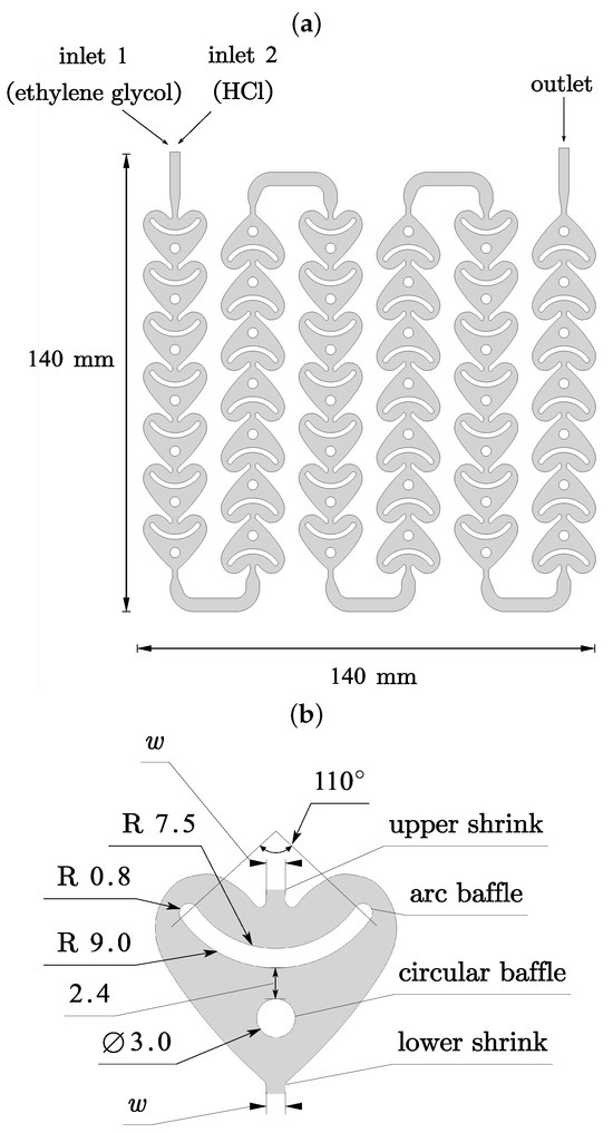
Figure 1.
The 2D diagram of Corning’s G1 micromixer. (a) All mixing units. (b) Single mixing unit.
Optimizations of two baffles and a heart-shaped profile in a single unit can considerably impact the mixing efficiency. However, the geometrical modification in such a configuration may raise new challenges in manufacturing. On the contrary, a simple alteration of microchannel width w is an economical alternative to optimize the mixing efficiency. Since the microchannel width is sensitive to molecular diffusion intensity and resistance time, the involved microchannel widths are designed in a range of 1.5–2.5 mm to search the compromised optimization in this study based on the original design of microchannel width of 1.5 mm. Considering the manufacturing challenges and pump head, the smaller width (<1.5 mm) is not yet considered in our current numerical study. Therefore, the microchannel width w, rather than other geometrical parameters, is discussed in this study.
As in experiments, two miscible and nonreactive fluids of ethylene glycol and hydrochloric acid (HCl, 37 wt%) were chosen to analyze the mixing processes and efficiency. Those two phases were initially pumped (under the same feed pressure p) into the assigned inlet. The mixing performance is indicated as , which is in terms of feed flow volume in this study (see Equations (9) and (10)). Furthermore, the feed flow volume is provided by the feed pressure of the pump. A relatively higher pressure (or high flow rate) will also benefit the vortex intensity, while the lower feed pressure condition has a longer residence time. Therefore, the feed pressure p is also investigated in this study.
According to the above considerations and industrial practice, three levels of feed pressure p (i.e., 0.1 MPa, 0.2 MPa, and 0.3 MPa) and eleven levels of microchannel width w (1.5–2.5 mm with an equal interval of 0.1 mm) were chosen in the simulations. In simulations, the feed pressure and 0 MPa were imposed on the inlet and outlet, respectively. All the micromixer inner walls were set as solid and no-slip. Table 1 displays the fundamental physical properties of the two fluids involved in the simulation.

Table 1.
Physical parameters of the two substances ().
2.1.3. Grid Independence Test
Due to the complex structure of the mixing unit, the unstructured mesh was used to solve the governing equations on the total computational domain (Figure 2). The fundamental mesh size is established considering the precision and efficiency of the computation.
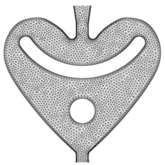
Figure 2.
The mesh of microchannel compute field.
The computational domain of the micromixer was meshed using a mixture of triangular and quadrilateral patterns. Four basic mesh sizes were used, namely 0.0375 mm, 0.075 mm, 0.15 mm, and 0.3 mm, with corresponding numbers of mesh cells from 118,000 to 1,114,000. The simulations at pressure inlet conditions of 0.1 MPa resulted in mass flux calculations of 2.155 kg/s, 2.163 kg/s, 2.296 kg/s, and 3.721 kg/s after flow stabilization, respectively. When the grid size is taken as 0.15 mm, there is a 6.5% deviation in the mass flux value compared to the smallest grid size, 0.0375 mm. However, the computational error is notably reduced when the number of grids is decreased by 77.1% to 255,000. When the grid is divided using 0.3 mm, the number of grids decreases to 118,000. However, the error in the mass flow value increases to 72.7%. Therefore, this paper uses a mesh size of 0.15 mm to ensure accurate results and reduce calculation time.
2.2. Optimization Strategy
2.2.1. Response Surface Method
The core of the RSM is to seek the best fit of an equation or expressions for the optimization objectives based on the experimental or simulation data. It enables statistical predictions to reduce the simulation time [22,23,24]. With its short cycle and high precision, RSM can fully capture the interactions between multiple factors.
Generally, RSA is divided into two stages:
(a) Use fitting methods such as least squares, kernel methods, spline methods, etc., to construct response surface functions based on experimental or simulation data;
(b) Analyze the importance of the effects using the model obtained, then optimize the model and look for the factor level combinations that give the maximum yield and minimum costs.
The validity of the fitted equations can be assessed using three additional performance evaluation metrics, such as Equations (6)–(8):
The sum of squared error (SSE),
The root mean squared error (RMSE) is,
and the coefficient of determination () is
where CFD values are denoted as , the response surface model value is denoted as , the average of CFD values is denoted as , and the number of samples is denoted as N. The response surface’s fitting accuracy is higher when RMSE and SSE are closer to 0 and is closer to 1.
2.2.2. Parallel Particle Swarm Algorithm
The particle swarm algorithm (PSO) is a stochastic optimization technique based on population, which utilizes a group of random initial solutions for finding the optimum solution through iterative processes [25]. PPSO enables information sharing on the optimal positions of all populations among multiple particle swarms [26,27,28,29]. After each iteration, the optimal position, generated from comparing all populations, becomes the optimal position of particles in all populations. Each particle uses it as the target for updating its position and velocity. Due to the implementation of the parallel mechanism, each population’s search efficiency has dramatically improved [30,31], leading the algorithm to converge to the optimal solution faster.
2.2.3. Optimization Goal and Steps
The optimization objective of this study is to maximize the mixing efficiency of the microchannel. Objective evaluation of fluid mixing effectiveness is typically based on several theoretical calculations, the most prevalent being the standard deviation approach. Standard deviation is a statistical concept used to measure the variability within data sets, and it can be applied to measure the degree of fluid mixing, where the mixing index can be expressed as follows [32,33]:
where is the volumetric concentration of a substance at each point in the field being counted; N is the number of statistical locations in the field being counted; and is the expected value of the concentration in the cross-section being counted,
where and are the volume flows of HCl and ethylene glycol pumped into the system. Specifically, if the real mixing reaches the expected condition, and for the immiscible flows or the mixing process is not activated. Since Equations (9) and (10) are derived in terms of constant feed flow volume, which can be applied to the mixing process of the incompressible continuous fluids. Additionally, the feed flow volume is propositional to the feed flow speed and feed time at the inlet microchannel. In contrast, the feed power of the pump is highly related to the fluid property (e.g., density, viscosity, and surface tension).
A monitoring line is established at the microchannel outlet to characterize the mixing efficiency in the numerical simulation of the fluid. The volume fraction of HCl for each grid on the monitoring line serves as the concentration component for that grid.
Our work mainly focuses on the effect of the channel’s central width and inlet pressure on the micromixer’s mixing performance. On the one hand, to take advantage of the molecular diffusion of microchannels, the width of microchannels should be small enough to increase the specific surface area to promote molecular diffusion and, on the other hand, to ensure the conveying speed of high-viscosity fluids to ensure that the width of the channel is sufficiently large; enough pressure can provide a higher average flow rate to generate enough vortex intensity to promote mixing. However, too high a pressure will reduce the mixing system’s stability and safety while generating high energy consumption simultaneously. Hence, the objective function is defined as:
The flowchart of the algorithm operation for microchannels’ width optimization is shown in Figure 3.
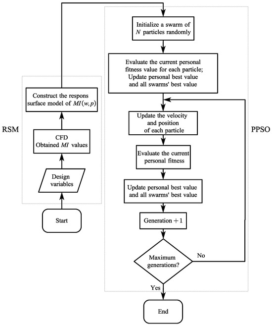
Figure 3.
Flowchart of algorithm operation for microchannel structural optimization.
3. Results and Discussion
3.1. Effect of the Feed Pressure
An increase in inlet pressure leads to an increase in flux. However, the mixing efficiency decreases as the pressure increases, as shown in Figure 4. The pressure loss increases along the length of the process. Factors impacting the micromixer’s pressure loss include resistance and local resistance loss. Specifically, the pressure loss includes fluid flow through the sharp corners and sudden expansion and contraction of the structure, turbulent kinetic energy loss, frictional resistance, pressure drag resistance from the baffles’ surfaces, and other forms of pressure loss.
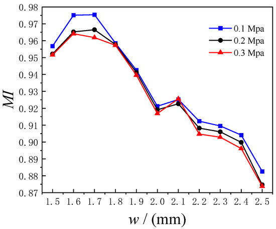
Figure 4.
The against the width.
Figure 5 displays the velocity and pressure distribution of the first mixing unit. When fluid flows through the narrow mouth, creating a low-pressure zone, the fluid flow velocity reaches the maximum at the shrink. Subsequently, the pressure increases as the flow expands through the more comprehensive section, and two additional low-pressure zones form in front of the arc baffle while a high-pressure zone is formed directly in front of the arc baffle. The liquid from the high-pressure zone recirculates into the two low-pressure zones to create two vortexes as a secondary flow occurs. When the fluid flows through the arc baffle, the fluid achieves relatively uniform flow pressure. It generates another secondary flow before the circular baffle, forming another vortex (see the first subfigure in Figure 6). Within the second shrink, velocity is at its highest while pressure reaches its minimum in the mixing unit.
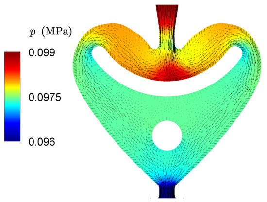
Figure 5.
The velocity vector and pressure of the first mixing unit under 0.1 MPa.
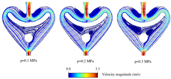
Figure 6.
The streamline of the first mixing unit under 0.1 MPa, 0.2 MPa, and 0.3 MPa.
Figure 6 displays the flow profile in the first mixing unit of a 1.5 mm wide microchannel under different pressure conditions, colored by velocity magnitude. The average flow velocity of the fluid in the channel rises as the feed pressure increases. As the pressure increases sequentially, the intensity of the two vortices in front of the arc baffle rises. At a pressure of 0.1 MPa, a single vortex is generated by the secondary flow in front of the circular baffle, whereas two vortices are formed in front of the circular baffle at both 0.2 MPa and 0.3 MPa. Additionally, the vortex size at 0.3 MPa is more significant than that at 0.2 MPa. For the same configuration, the average flux within the channel increases with the inlet pressure. When the flux is too high, the fluid in the flow channel inside the flow time is limited, resulting in a shorter distance for molecular lateral diffusion, which leads to insufficient molecular mixing. Conversely, when the flux is too low, the fluid flows smoothly, and there is less collision between the fluid molecules, making producing the necessary eddy effects challenging. This limited convective shear between the fluid also hampers the mixing efficiency of the fluid.
The combined effects of the two factors below influence the pressure’s impact on mixing efficiency. The numerical results of the mixing index decreasing with increasing pressure demonstrates that enhanced mixing efficiency through diffusion resulting in a vortex via increased velocity is less effective than the reduction of mixing efficiency affected by molecular diffusion. This conclusion is consistent with [34,35,36]. In addition, a microchannel width that is too wide reduces molecular diffusion efficiency, while a width that is too narrow increases along-travel resistance.
3.2. Effect of the Channel Width
The impact of channel width on the mixing index is significant, as displayed in Figure 4. When the inlet pressure is fixed, the mixing index is non-monotonic with the microchannel width. A reasonable explanation is as follows.
As the width of the microchannel increases, it reduces resistance and weakens the boundary layer effect, leading to an increase in average flux, which may intensify the collisions between fluids. However, when the flux is too high, the fluid travels quickly through the channel, causing the lateral diffusion distance between molecules to decrease, which leads to uneven mixing.
Conversely, the fluid travels smoothly without intense collisions between molecules when the flux is too low. This is adverse to producing a vortex and so reduces fluid mixing efficiency. Therefore, for the same pressure in the microchannel, the impact of the microchannel width on mixing performance is the combination of the following two factors:
- The negative impact due to the reduction of the total flow time, which decreases the diffusion intensity of free molecules;
- The positive factor is due to the increased eddy intensity, which contributes to the vortex diffusion performance.
The CFD results in Figure 4 show that, as the channel width increases, the mixing index increases first and then decreases.
3.3. Response Surface Model of Mixing Index
The scatter distribution of the mixing index was obtained (Figure 4) according to the CFD results and Equation (9). In this section, a customized function is constructed to express the relationship between the mixing index and the channel width accompanied by inlet pressure.
Figure 4 shows that, when inlet pressure p is fixed, the relationship curve between the mixing index and channel width w is approximately parallel. This implies that the nonlinear correlation between the mixing index and channel width at a fixed pressure should be established first to construct the overall response surface function.
Figure 7 shows a scatter plot and fitting curve of the mixing index with the channel width under 0.1 MPa. It was found that the 5th-degree polynomial provides the best regression accuracy. The coefficients are determined by the least square method, and the coefficient of determination, (Equation (8)), is 0.990. The expression is as follows:
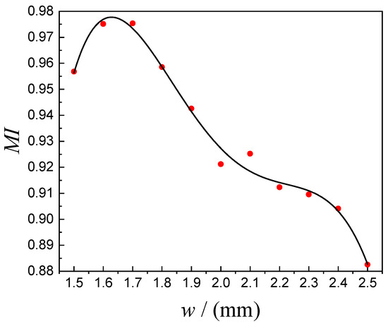
Figure 7.
Scatter plot of mixing index versus channel width under 0.1 MPa.
From the parallel relationship of curves between the mixing index and channel width shown in Figure 4, it can be inferred that the mixing index response surface equation includes the 5th-degree polynomial. The relationship is expressed as:
where is a set of coefficients determined by the least square method based on all CFD results in this study (see Table 2), and p is the inlet pressure.
Table 2.
Coefficients of response surface function of .
Figure 8 depicts the mixing index variation concerning channel width and inlet pressure calculated by the fitting equation. Notably, CFD values close to the response surface of indicate that the construction method of the response surface is reasonable. Table 3 shows the performance evaluation indexes of the mixing index response surface model. The coefficient of determination of the response surface equation for the mixing efficiency index is 0.98221.
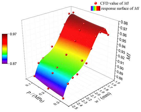
Figure 8.
The CFD value scatter plot and response surface of mixing index against the width and pressure.
Table 3.
Evaluation indexes of the mixing index response surface model.
3.4. Microchannel Width Optimization by PPSO
From the above, it is evident that the optimal central width of the micromixer for achieving the maximum mixing index of the miscible liquid–liquid system is consistent across all pressure ranges from 0.1 MPa to 0.3 MPa. The max will occur under 0.1 MPa. Therefore, we utilize PPSO [30] based on the Equation (12) to get the optimal channel width. The PPSO program sets 20 parallel populations, each with 20 particles, and a maximum iteration limit of 200. The iterative fitness curve of the algorithm is shown in Figure 9, and it is observed that the fitness reaches its optimal value after seven generations, corresponding to a maximum mixing index of 0.9827, with the populations reaching the optimal position of 1.634 mm.
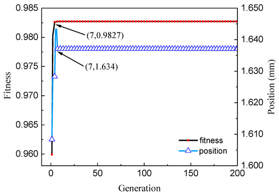
Figure 9.
Maximum fitness curve and best position curve under 0.1 MPa based on Equation (12).
3.5. CFD Verification of Optimization Results
The numerical model of a microchannel with a 1.634 mm width is fabricated for CFD simulation and analysis at 0.1 MPa, 0.2 MPa, and 0.3 MPa. Figure 10 shows the HCl volume fraction of the first mixing unit with different widths, i.e., 1.5 mm and 1.634 mm, and it is obvious that two fluids mix more evenly in the 1.634 mm mixing unit. Table 4 compares the CFD simulation’s experimental values with the calculated values of the response surface model.
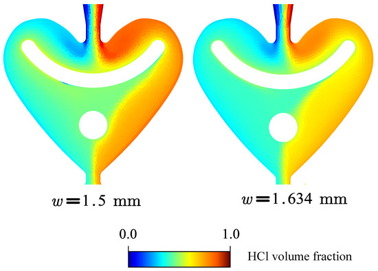
Figure 10.
The HCl volume fraction of the first mixing unit with a width of 1.5 mm and 1.634 mm.
Table 4.
Comparison of 1.634 mm wide microchannel flux and mixing index of RSM-predicted values with CFD values.
It can be seen that, under the three inlet pressures, the response surface predictions and CFD simulations of the mixing index agree well, and the average relative error is 1.57%. In contrast, the flux consistency is not as good as the mixing index, with an average relative error of 2.93%.
The optimized 1.634 mm microchannel improves the mixer’s flux and mixing efficiency compared to the original design of Corning’s G1 mixer, i.e., a 1.5 mm mixer, variant at 0.1 MPa, 0.2 MPa, and 0.3 MPa. On average, the flux is increased by 13.51%, and mixing efficiency is increased by 2.45% (see Table 5). These results demonstrate the effectiveness of the optimized micromixer in enhancing the flux and mixing efficiency of miscible liquid–liquid two-phase mixtures.
Table 5.
Comparison of CFD values between 1.634 mm and 1.5 mm wide microchannels under different inlet pressures.
4. Conclusions
The simulation of miscible liquid–liquid two-phase flow in a Corning G1 micromixer was achieved using the mixture model. The microchannel’s feed pressure and central width effect on the flux and mixing efficiency were analyzed. A response surface model for the mixing index was subsequently proposed.
- The most effective width for the channel and its associated mixing index were determined using PPSO for the response surface model. Those values were 1.634 mm and 0.9827, respectively. The numerical model of the micromixer was designed using the optimized parameter and was verified with CFD. The CFD values agree with the predicted values of the response surface model well, and their average relative errors for the flux and mixing index are 2.93% and 1.09%, respectively.
- The optimized 1.634 mm microchannel improves the mixer’s flux and mixing efficiency of miscible liquid–liquid mixtures compared to the original Corning’s G1 mixer, i.e., the mixer with a 1.5 mm width under the pressure variant at 0.1 MPa, 0.2 MPa, and 0.3 MPa. On average, the flux increases by 13.51%, and mixing efficiency improves by 2.45%.
Besides the channel width, the key structural parameters of the arc baffle and cylindrical baffle, etc., may also affect the mixing performance of the G1 micromixer [37,38]. However, modifications of these structure parameters usually introduce manufacturing challenges and costs. On the contrary, a few studies [39,40,41] have reported that the mixing performance is also sensitive to the microchannel width (w), so simple modifications of the channel width may increase the mixing performance significantly. This study discusses the effects of microchannel width and feed pressure on mixing performance rather than other structural and manipulation parameters. The research interest specifically focuses on the mixing performance of HCl and ethylene glycol solutions. Although this work is based on a specific design and process, the workflow in this paper can provide the standard processing for optimizing other flow mixers.
Author Contributions
Conceptualization, L.L.; methodology, X.L.; software, L.Q.; validation, L.Q., X.L. and H.H.; formal analysis, H.H. and X.Y.; investigation, M.C., H.H. and X.Y.; resources, L.Q.; data curation, M.C., X.Y. and W.M.; writing—original draft preparation, L.Q. and H.H.; writing—review and editing, L.Q., H.H. and H.W.; visualization, M.C., S.C. and H.H.; supervision, X.L. and L.L.; project administration, L.L. All authors have read and agreed to the published version of the manuscript.
Funding
This research was partially funded by the China Postdoctoral Science Foundation (2022M711766).
Institutional Review Board Statement
Not applicable.
Informed Consent Statement
Not applicable.
Data Availability Statement
Data are contained within the article.
Conflicts of Interest
The authors declare no conflicts of interest. The funders had no role in the design of the study; in the collection, analyses, or interpretation of data; in the writing of the manuscript; or in the decision to publish the results.
Abbreviations
The following abbreviations are used in this manuscript:
| CFD | computational fluid dynamics |
| PPSO | parallel particle swarm optimization |
| RSM | response surface methodology |
| LOC | lab on a chip |
| coefficient of determination | |
| RMSE | root mean squared error |
| SSE | sum of squared error |
| mixing index | |
| w | width of microchannel |
| hydraulic diameter | |
| density of the mixture | |
| viscosity of mixture | |
| mass-averaged velocity | |
| volume fraction of the phase | |
| Reynold number | |
| drift velocity of the second phase | |
| density of fluid | |
| viscosity of fluid | |
| velocity at the channel surface | |
| volumetric concentration of the ethylene glycol at each measured point on the cross-section | |
| expected value of the concentration | |
| volumetric flux of the HCl | |
| volumetric flux of the ethylene | |
| p | inlet pressure |
| CFD calculated values | |
| response surface model value | |
| average of CFD calculated values | |
| mixing index model coefficient |
References
- Sarsfield, M.; Roberts, A.; Streletzky, K.A.; Fodor, P.S.; Kothapalli, C.R. Optimization of gold nanoparticle synthesis in continuous-flow micromixers using response surface methodology. Chem. Eng. Technol. 2021, 4, 622–630. [Google Scholar] [CrossRef]
- Wangikar, S.S.; Patowari, P.K.; Misra, R.D.; Gidde, R.R.; Bhosale, S.B.; Parkhe, A.K. Optimization of photochemical machining process for fabrication of microchannel with obstacles. Mater. Manuf. Process. 2020, 12, 544–557. [Google Scholar] [CrossRef]
- Raza, W.; Ma, S.B.; Kim, K.Y. Single and multi-objective optimization of a three-dimensional unbalanced split-and-recombine micromixer. Micromachines 2019, 10, 711. [Google Scholar] [CrossRef] [PubMed]
- Nguyen, N.T.; Wu, Z. Micromixers—A review. J. Micromech. Microeng. 2005, 15, R1. [Google Scholar] [CrossRef]
- Myachin, I.V.; Kononov, L.O. Mixer design and flux as critical variables in flow chemistry affecting the outcome of a chemical reaction: A review. Inventions 2023, 8, 128. [Google Scholar] [CrossRef]
- Natsuhara, D.; Saito, R.; Okamoto, S.; Nagai, M.; Shibata, T. Mixing performance of a planar asymmetric contraction-and-expansion micromixer. Micromachines 2022, 13, 1386. [Google Scholar] [CrossRef] [PubMed]
- Saravanakumar, S.M.; Cicek, P.-V. Microfluidic mixing: A physics-oriented review. Micromachines 2023, 14, 1827. [Google Scholar] [CrossRef] [PubMed]
- Kassin, V.E.H.; Toupy, T.; Petit, G.; Bianchi, P.; Salvadeo, E.; Monbaliu, J.C.M. Metal-free hydroxylation of tertiary ketones under intensified and scalable continuous flow conditions. J. Flow Chem. 2020, 10, 167–179. [Google Scholar] [CrossRef]
- Chen, Y.; Chen, X. An improved design for passive micromixer based on topology optimization method. Chem. Phys. Lett. 2019, 734, 136706. [Google Scholar] [CrossRef]
- Lv, H.; Chen, X.; Zeng, X. Optimization of micromixer with cantor fractal baffle based on simulated annealing algorithm. Chaos Solitons Fractals 2021, 148, 111048. [Google Scholar] [CrossRef]
- Hossain, S.; Ansari, M.A.; Husain, A.; Kim, K.Y. Analysis and optimization of a micromixer with a modified tesla structure. Chem. Eng. J. 2010, 4, 305–314. [Google Scholar] [CrossRef]
- Zhang, J.; Guo, W.; Xie, Z.; Guan, X.; Qu, X.; Ge, Y. Optimization of fin layout in liquid-cooled microchannel for multi-core chips. Case. Stud. Therm. Eng. 2023, 41, 102615. [Google Scholar] [CrossRef]
- Freeny, A. Empirical model building and response surfaces. Technometrics 1988, 5, 229–231. [Google Scholar] [CrossRef]
- Obregón, D.; Hadzich, A.; Bellatin, L.; Flores, S. Microwave-assisted synthesis of alkyd resins using response surface methodology. Chem. Eng. Process. 2023, 183, 109221. [Google Scholar] [CrossRef]
- Zahran, H.A.; Catalkaya, G.; Yenipazar, H.; Capanoglu, E.; Şahin-Yeşilçubuk, N. Determination of the optimum conditions for emulsification and encapsulation of echium oil by response surface methodology. ACS Omega 2023, 8, 28249–28257. [Google Scholar] [CrossRef] [PubMed]
- Yang, R.; Li, W.; Liu, Y. A novel response surface method for structural reliability. AIP Adv. 2022, 12, 015205. [Google Scholar] [CrossRef]
- Berger, P.D.; Maurer, R.E.; Celli, G.B. Experimental Design: With Applications in Management, Engineering, and the Sciences, 2nd ed.; Springer International Publishing: Cham, Switzerland, 2018; pp. 533–584. [Google Scholar]
- Manninen, M.; Taivassalo, V.; Kallio, S. On the Mixture Model for Multiphase Flow; VTT Publications: Espoo, Finland, 1996; pp. 16–18. [Google Scholar]
- Massoudi, M. Boundary conditions in mixture theory and in CFD applications of higher order models. Comput. Math. Appl. 2007, 53, 156–167. [Google Scholar] [CrossRef]
- Járvás, G.; Quellet, C.; Dallos, A. Cosmo-rs based cfd model for flat surface evaporation of non-ideal liquid mixtures. Int. J. Heat Mass Transfer 2011, 54, 4630–4635. [Google Scholar] [CrossRef]
- Fang, Z.; Hou, W.; Xu, Z.; Guo, X.; Zhang, Z.; Shi, R.; Yao, Y.; Chen, Y. Large eddy simulation of cavitation jets from an organ-pipe nozzle The influence of cavitation on the vortex coherent structure. Processes 2023, 11, 2460. [Google Scholar] [CrossRef]
- Robinson, D. Statistical design: Chemometrics. Org. Process Res. Dev. 2006, 9, 1082–1083. [Google Scholar] [CrossRef]
- Li, P.; Huang, C.; Hu, S.; Yang, S.; Wen, H.; Zhou, L. Efficient sparse representation response surface modeling and simulation method for complex products. Mater. Sci. Eng. 2018, 436, 012005. [Google Scholar]
- Xia, Y.; Wang, Y. Improved hybrid response surface method based on double weighted regression and vector projection. Math. Probl. Eng. 2022, 17, 5104027. [Google Scholar] [CrossRef]
- Kennedy, J.; Eberhart, R. Particle swarm optimization. In Proceedings of the International Conference on Neural Networks, Perth, Australia, 27 November–1 December 1995. [Google Scholar]
- Desmarais, J.K.; Spiteri, R.J. Fast automated airborne electromagnetic data interpretation using parallelized particle swarm optimization. Comput. Geosci. 2017, 109, 268–280. [Google Scholar] [CrossRef]
- Gao, Z.; Yu, J.; Zhao, A.; Hu, Q.; Yang, S. Optimal chiller loading by improved parallel particle swarm optimization algorithm for reducing energy consumption. Int. J. Refrig. 2022, 136, 61–70. [Google Scholar] [CrossRef]
- Li, B.; Wada, K. Parallelizing particle swarm optimization. In Proceedings of the IEEE Pacific Rim Conference on Communications, Computers and Signal Processing, Victoria, BC, Canada, 24–26 August 2005. [Google Scholar]
- Li, M.; Huang, L.; Xu, G.; Biao, K. A parallel particle swarm optimization framework based on a fork-join thread pool using a work-stealing mechanism. Appl. Soft. Comput. 2023, 145, 110537. [Google Scholar] [CrossRef]
- Gad, A.G. Particle swarm optimization algorithm and its applications: A systematic review. Arch. Comput. Methods Eng. 2022, 29, 2531–2561. [Google Scholar] [CrossRef]
- He, Z.; Xiong, X.; Yang, B.; Li, H. Aerodynamic optimisation of a high-speed train head shape using an advanced hybrid surrogate-based nonlinear model representation method. Optim. Eng. 2022, 23, 59–84. [Google Scholar] [CrossRef]
- Chen, X.; Zhao, Z. Numerical investigation on layout optimization of obstacles in a three-dimensional passive micromixer. Anal. Chim. Acta 2017, 964, 142–149. [Google Scholar] [CrossRef]
- Shen, B.; Zhan, X.; Sun, Z.; He, Y.; Long, J.; Li, X. Piv experiments and cfd simulations of liquid–liquid mixing in a planetary centrifugal mixer (pcm). Chem. Eng. Sci. 2022, 9, 259. [Google Scholar] [CrossRef]
- Yoshimura, M.; Shimoyama, K.; Misaka, T.; Obayashi, S. Optimization of passive grooved micromixers based on genetic algorithm and graph theory. Microfluid. Nanofluid. 2019, 23, 30. [Google Scholar] [CrossRef]
- Gonçalves, I.M.; Castro, I.; Barbosa, F.; Faustino, V.; Catarino, S.O.; Moita, A.; Miranda, J.M.; Minas, G.; Sousa, P.C.; Lima, R. Experimental characterization of a microfluidic device based on passive crossflow filters for blood fractionation. Processes 2022, 10, 2698. [Google Scholar] [CrossRef]
- Chen, X.; Li, T. A novel passive micromixer designed by applying an optimization algorithm to the zigzag microchannel. Chem. Eng. J. 2017, 313, 1406–1414. [Google Scholar] [CrossRef]
- Mirkarimi, S.M.H.; Hosseini, M.J.; Pahamli, Y. Numerical investigation of a curved micromixer using different arrangements of cylindrical obstacles. Alex. Eng. J. 2023, 79, 135–154. [Google Scholar] [CrossRef]
- Wang, X.; Liu, Z.; Wang, B.; Cai, Y.; Song, Q. An overview on state-of-art of micromixer designs, characteristics and applications. Anal. Chim. Acta 2023, 1279, 341685. [Google Scholar] [CrossRef] [PubMed]
- Bernacka-Wojcik, I.; Ribeiro, S.; Wojcik, P.J.; Alves, P.U.; Busani, T.; Fortunato, E.; Baptista, P.V.; Covas, J.A.; Águas, H.; Hilliou, L.; et al. Experimental optimization of a passive planar rhombic micromixer with obstacles for effective mixing in a short channel length. RSC Adv. 2014, 4, 56013–56025. [Google Scholar] [CrossRef]
- Afzal, A.; Kim, K.-Y. Optimization of pulsatile flow and geometry of a convergent–divergent micromixer. Chem. Eng. J. 2015, 281, 134–143. [Google Scholar] [CrossRef]
- Das, S.S.; Tilekar, S.D.; Wangikar, S.S.; Patowari, P.K. Numerical and experimental study of passive fluids mixing in micro-channels of different configurations. Microsyst. Technol. 2017, 23, 5977–5988. [Google Scholar] [CrossRef]


Disclaimer/Publisher’s Note: The statements, opinions and data contained in all publications are solely those of the individual author(s) and contributor(s) and not of MDPI and/or the editor(s). MDPI and/or the editor(s) disclaim responsibility for any injury to people or property resulting from any ideas, methods, instructions or products referred to in the content. |
© 2024 by the authors. Licensee MDPI, Basel, Switzerland. This article is an open access article distributed under the terms and conditions of the Creative Commons Attribution (CC BY) license (https://creativecommons.org/licenses/by/4.0/).