1. Introduction
The hybrid flow shop scheduling problem (HFSP), which combines the features of traditional flow shop scheduling and parallel machine scheduling, is widely employed in the auto industry, food processing, steel forging [
1], and other industries. The HFSP buffer is always intended to be infinite; however, owing to product processes and technological restrictions, the buffer is sometimes non-existent or confined. As a result, when all the machines in the following stage are in the processing state, the jobs processed in the previous stage will be blocked on the present machine until an idle machine in the next stage becomes available [
2]. This is referred to as the blocking hybrid flow shop scheduling problem (BHFSP). Blocking increases the waiting time for jobs, resulting in a longer makespan and an increase in energy consumption, both of which have an influence on production efficiency. With increased worldwide environmental consciousness and the implementation of China’s carbon peak and carbon neutrality goals, energy consumption is increasingly being emphasized as a critical green production metric for enterprises. At the same time, the transportation time of materials between different stages in the process industry cannot be ignored. As a result, in the production of hybrid flow shops, considering the impact of blocking, coordinating production, transportation times, and energy consumption, drawing up production plans can efficiently utilize resources, reduce production costs, and enhance enterprise competitiveness.
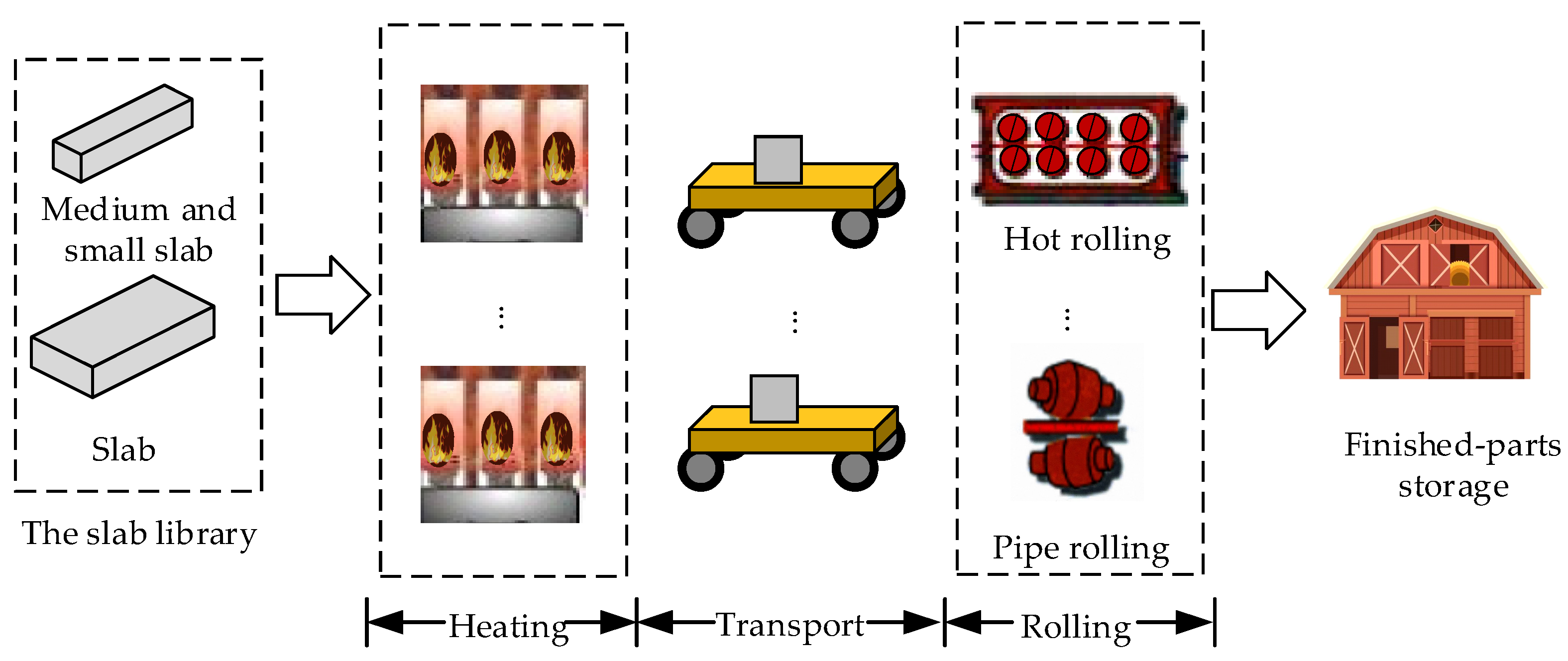
We take the heating–rolling stage in a steel enterprise as an example. When there is a need for processing, the slab is first heated in the heating furnace and then transported by trolley to the rolling stage. Steel rolling includes hot rolling, tube rolling, structural steel rolling, and wire rolling, etc. Semi-finished slabs will be blocked in the heating furnace for insulation when the slab is heated in the heating furnace and all the machines in the rolling stage are in processing mode to prevent material deterioration. The job blocking on machines can lead to energy waste and delay the delivery time. Therefore, a multi-objective scheduling problem for a hybrid flow shop considering transportation time was refined by jointly considering economic and green indicators.
Figure 1 depicts the process flowchart for the heating–rolling stage.
From the past to the present, the majority of scholars have focused on researching the blocking flow shop scheduling problem (BFSP). Du et al. [
3] investigated a distributed BFSP with an assembly machine and optimized it for total assembly completion time. They proposed an effective discrete monarch butterfly optimization algorithm. Miyata et al. [
4] aimed to minimize the total completion time subject to total maintenance costs in BFSP and introduced a mixed-integer linear programming method to solve the problem. Cheng et al. [
5] aimed to minimize the total completion time and proposed an effective metaheuristic algorithm to solve BFSP with sequence-dependent setup times. Zhao et al. [
6] studied the distributed assembly BFSP with the total tardiness criterion and employed a mixed-integer linear programming approach for problem modeling. They introduced a constructive heuristic algorithm and a water wave optimization algorithm based on problem-specific knowledge. Niu et al. [
7] addressed the distributed group BFSP with carryover sequence-dependent setup time constraints. They proposed a two-stage cooperative coevolutionary algorithm aiming to minimize the makespan and total energy consumption. Zhao et al. [
8] investigated the distributed BFSP with sequence-dependence, taking into account makespan, total tardiness, and total energy consumption. They introduced a cooperative whale optimization algorithm for solving this problem. Bao et al. [
9] focused on the sequence-dependent BFSP with energy-aware considerations and constructed a mixed-integer linear programming model to minimize makespan and total energy consumption. They proposed a cooperative iterated greedy algorithm based on Q-learning. Nagano et al. [
10] addressed the permutation flow shop problem with process blocking and setup times and presented an improved branch-and-bound algorithm with the objective of minimizing total flow time and tardiness. However, traditional flow shop scheduling lacks flexibility, and production lines are often singular. In contrast, the BHFSP allows for one or more parallel machines at each operation, providing adaptability to various production tasks. This not only reduces costs for enterprises but also enhances production efficiency.
Many researchers have conducted studies on HFSP with blocking constraints in recent years. Wang et al. [
11] proposed a hybrid decode-assisted mutation iterative greedy algorithm for BHFSP with the objective of minimizing the makespan. Qin et al. [
12] proposed a mathematical model of BHFSP based on energy-saving criteria and an improved iterative greedy algorithm based on an exchange strategy to minimize total energy consumption. Shao et al. [
13] studied the distributed heterogeneous BHFSP, where the objective function is to minimize the makespan, and proposed a learning-based selection hyper-heuristic framework. Missaoui et al. [
14] studied BHFSP where the objective function is to minimize the sum of weighted earliness and tardiness and proposed an efficient iterated greedy approach. Aqil et al. [
15] studied BHFSP under the constraint of sequence-dependent setup time where the objective function is to minimize the total tardiness and earliness and proposed six algorithms based on the migratory bird optimization and water wave optimization. Qin et al. [
16] established a mathematical model of BHFSP, where the objective is to minimize the makespan, and designed an iterative greedy algorithm with a double-level mutation strategy. Zhao et al. [
17] proposed a cooperative monarch butterfly optimization algorithm to solve the distributed assembly blocking flow shop scheduling problem, where the optimization objective is to minimize the assembly completion time. Wang et al. [
18] investigated the BHFSP on batch processing machines. Their objective was to minimize the total energy consumption of machines and the makespan. They designed a hybrid meta-heuristic algorithm based on ant colony optimization and genetic algorithms to solve this problem. It can be observed that most research on BHFSP primarily focuses on single-objective optimization, where the main optimization objectives are makespan, tardiness, or energy consumption. In light of the increasingly severe environmental challenges, the consideration of coordinated optimization among multiple objectives, such as completion time and energy consumption, is not only crucial for enhancing economic benefits for enterprises but also contributes to achieving sustainable development goals and alleviating environmental burdens.
In the research on multi-objective HFSP, Feng et al. [
19] studied HFSP based on the parallel sequential movement mode, where the optimization objective is to maximize both the makespan and handling events, and proposed an improved non-dominated sorting genetic algorithm (NSGA-II) to find Pareto solutions. Lei et al. [
20] focused on the optimization objectives of minimizing the makespan and maximizing the tardiness and designed an optimization algorithm based on multi-class teaching to solve the distributed HFSP with sequence-dependent setup times. Geng et al. [
21] aimed to minimize the makespan and maximize the average agreement index and designed a hybrid NSGA-II algorithm to solve the fuzzy re-entrant HFSP. Wu et al. [
22] studied the re-entrant HFSP with continuous batch processing machines and proposed an improved multi-objective evolutionary algorithm based on decomposition to reduce the production cycle and energy consumption in the production of cold-drawn seamless steel pipes. Wang et al. [
23] aimed to minimize the makespan, the total energy consumption, and the processing cost of the machine and proposed an improved decomposition-based multi-objective evolutionary algorithm to solve the HFSP. Song et al. [
24] aimed to minimize both the energy consumption and the makespan and proposed an improved fast NSGA-II to solve the HFSP. Lei et al. [
25] solved the distributed two-stage HFSP considering sequence-dependent setup times and proposed an improved shuffled frog leaping algorithm to minimize the number of tardy jobs and the makespan simultaneously. Song et al. [
26] aimed to minimize completion time and energy consumption and proposed a hybrid multi-objective teaching–learning-based optimization algorithm based on decomposition to solve the HFSP with an unrelated parallel machine. Li et al. [
27] investigated energy-efficient HFSP with uniform machines and formulated a new multi-objective mixed-integer nonlinear programming model to minimize total tardiness, total energy cost, and carbon trading cost. They introduced the NSGA-II based on Q-learning and general variable neighborhood search. Wang et al. [
28] explored HFSP with dynamic reconfiguration processes and the dual objectives of minimizing the makespan and the whole device’s energy consumption. They obtained a Pareto-based optimal solution set using an improved multi-objective whale optimization algorithm. Cui et al. [
29] studied a multi-objective HFSP with unrelated parallel machines, considering minimum makespan and total tardiness, and designed an enhanced multi-population genetic algorithm for solution optimization. In summary, it is essential to consider the impact of transportation time on scheduling results in the context of multi-objective HFSP.
Traditional HFSP solving methods often employ intelligent optimization algorithms and heuristic algorithms. For complex shop scheduling problems that are difficult to solve, reinforcement learning can learn the optimal strategy through interaction with the environment, and its application in the field of scheduling is becoming increasingly widespread. Currently, reinforcement learning has been researched in various settings, including single machines [
30], parallel machines [
31], flow shops [
32,
33], job shops [
34,
35], and flexible job shops [
36]. Particularly in the context of reinforcement learning for solving multi-objective problems, Zhang et al. [
37] conducted research on the distributed HFSP with a certain degree of symmetry. The objective is to minimize both the makespan and the number of tardy jobs and propose a dual-population genetic algorithm based on Q-learning. Cheng et al. [
38] designed a multi-objective Q-learning hyper-heuristic algorithm based on Bi-criteria selection, where the objective is to optimize both production efficiency and energy consumption simultaneously. Chang et al. [
39] studied the multi-objective dynamic flexible job shop scheduling problem (MODFJSP) and proposed a hierarchical reinforcement learning approach to solve the MODFJSP considering the arrival of random jobs. Li et al. [
40] conducted research on the multi-objective flexible job shop scheduling problem with fuzzy processing times, where the optimization objectives are makespan and total machine workload, and proposed a reinforcement learning-based multi-objective optimization algorithm. Yuan et al. [
41] studied the multi-objective optimization scheduling problem in heterogeneous cloud environments and proposed a multi-objective reinforcement learning job scheduling method with AHP-based weighting. Wu et al. [
42] studied the green dynamic multi-objective scheduling problem in a re-entrant hybrid flow shop and proposed an improved Q-learning algorithm. To sum up, when dealing with multi-objective problems, reinforcement learning algorithms typically employ a weighted summation of multiple objectives to transform them into a single objective. Objective weights are typically determined according to expert experience or experimentation. However, fixed weights are challenging to adapt in real time to changes in the state of the problem, thereby affecting the quality of the solutions.
As mentioned above, previous research in BHFSP has predominantly focused on single-objective optimization, with limited consideration for the coordinated transportation between upstream and downstream. Since the machines are at different geographical locations, transportation times have an impact on scheduling systems. Moreover, optimizing a single objective has inherent limitations when dealing with complex and diverse problems. Therefore, this paper investigates a multi-objective scheduling problem in a two-stage blocking hybrid flow shop with transportation constraints. In multi-objective optimization, determining objective weights often relies on expert experience or experiments. However, fixed weights are challenging to adapt in real time to changes in problem states, affecting the quality of solutions. This paper introduces a Q-learning algorithm based on adaptive objective selection. The algorithm better adapts to dynamic problem changes, enhancing solution flexibility and robustness. The detailed contributions of this paper are as follows:
- (1)
For the problem of modern industrial process manufacturing, due to production process requirements, downstream machine congestion can result in upstream blocking, and the transportation time between upstream and downstream cannot be ignored. This paper formulates the HFSP with both transportation and blocking constraints. With the optimization objectives of minimizing the makespan and the total energy consumption, a two-stage BHFSP model incorporating transportation is established.
- (2)
We have designed an improved multi-objective Q-learning algorithm to address this model. Additionally, an adaptive object selection strategy based on t-tests has been developed for handling multi-objective optimization problems. This strategy coordinates the selection of different objectives by evaluating the confidence of the objective functions under the current job and machine state, thus optimizing both completion time and energy consumption indicators effectively.
The rest of this paper Is organized as follows:
Section 2 establishes the mathematical model of the two-stage BHFSP with transportation times.
Section 3 describes the implementation details of the Q-learning algorithm based on adaptive object selection. In
Section 4, numerical experiments are conducted to demonstrate the effectiveness of the proposed algorithm. Finally, in
Section 5, conclusions are drawn, and future research directions are proposed.
2. Problem Formulation
The two-stage BHFSP with transportation times can be described as follows: There are n jobs that need to go through s (s = 1, 2) processing stages, each of which has multiple identical parallel machines, and each machine is located at a different geographical location. The processing sequence for all jobs is the same, and each job can be processed on any machine at each stage. The jobs processed in the first stage are transported to the production machines in the next stage by the transport vehicles. There is no buffer between stages, meaning that once a job completes its processing in the previous stage, it can only leave the machine when the next stage has available machines. The waiting time of the job is referred to as the blocking time. The objective function is to minimize both the makespan and the total energy consumption.
We assume that:
- (1)
All jobs have arrived at time zero and can begin processing.
- (2)
There is no limit to the number of transport vehicles that can be used after the job leaves the first-stage machine.
- (3)
Once the job begins processing or transporting, it cannot be interrupted.
The parameters and decision variables are defined as follows:
J: set of jobs, J = {1, 2, …, n};
Ms: set of machines, Ms = {1, 2, …, ms};
j: index of a job, j = 1, 2, …, n;
i: index of the first-stage machine, i = 1, 2, …, m1;
k: index of the second-stage machine, k = 1, 2, …, m2;
psj: the processing time of job j at stage s;
tik: the transportation time of the job from machine i to machine k;
SPi: the blocking power of a job on machine i in the first stage per unit of time;
TPik: the transportation power of a job from machine i to machine k per unit of time;
M: the large positive number;
Aj: the arrival time of job j;
Bsj: the start time of job j at stage s;
Csj: the completion time of job j at stage s;
L1j: the leave time of job j in the first stage;
π: the feasible overall scheduling solution;
tj(π): the transportation time of job j under the scheduling solution π;
wj(π): the waiting time of job j before processing in the first stage under the scheduling solution π;
bj(π): the blocking time of job j on the first-stage machine under the scheduling solution π;
Cmax: the makespan of job j;
TEC: the total energy consumption;
Xij: it is equal to 1 if job j is processed on machine i; otherwise, it is equal to 0;
Yjk: it is equal to 1 if job j is processed on machine k; otherwise, it is equal to 0;
Makespan: The factors affecting the completion time of the job include processing time, transportation time, waiting processing time, and blocking time. The formula is defined as follows:
where Equation (1) represents the objective function to minimize the makespan. Equation (2) defines the completion time of job
j as the sum of processing time, transportation time, waiting processing time, and blocking time. Equation (3) represents the transportation time of job
j. Equation (4) defines the waiting processing time of job
j before the first stage as the difference between its start processing time in the first stage and its arrival time. Equation (5) defines the blocking time of job
j on the first-stage machine as the difference between its leave time on the first-stage machine and its completion time.
- 2.
Total energy consumption: TEC includes blocking energy consumption (EC1), transportation energy consumption (EC2), and processing energy consumption (EC3). Notably, EC3 for each job is solely dependent on its processing time. Since each stage is equipped with identical parallel machines, EC3 is not affected by different processing sequences and remains constant. Therefore, Equation (6) shows that minimizing TEC requires minimizing EC1 and EC2. The second objective function is as follows:
where Equation (7) defines
EC1 as the energy consumed when a job is blocked on a machine. It is equal to the product sum of the blocking time of the job and the corresponding blocking power of the machine. Equation (8) defines
EC2 as the energy consumed when a vehicle transports a job. It is equal to the product of the transportation time of the job and the transportation power.
The following mathematical model is established based on the above problems:
s.t
where Equation (9) is the objective function and Equations (10)–(16) are constraints. Equation (10) represents a job that can only be processed by one machine at each stage. Equations (11) and (12) define the completion time of a job as the sum of its start processing time and its processing time. Equations (13) and (14) represent blocking constraints. Equation (13) defines the start processing time of a job in the second stage as the sum of its transportation time and its leave time in the first stage. Equation (14) represents when the start time of the latter processing job
j′ on the same machine cannot be shorter than the leave time of the former processed job
j. Equation (15) represents a job that can only leave after the operation is finished. Equation (16) represents when the start processing time of a job must be greater than or equal to 0. Equations (17) and (18) represent constraints on decision variables.
3. Adaptive Objective Selection Q-Learning Algorithm
The two-stage BHFSP model with transportation time established in
Section 2 is formulated as a multi-objective mixed-integer programming model. HFSP has been proven to be an NP-hard problem [
43], and due to the complexity of the problem studied in this paper, it is also NP-hard. Reinforcement learning enables autonomous learning through interaction between agents and the environment. It can adapt to diverse tasks and environments while achieving continuous improvement, giving it an advantage in intelligent decision-making and scheduling. In this section, an adaptive objective selection Q-learning algorithm (AQL) for solving multi-objective scheduling problems is designed. The confidence of the two objective functions is computed using a t-test, allowing for a focus on optimizing the object with the highest confidence.
3.1. Problem Transformation
3.1.1. State
The state feature mainly shows the environmental features of the blocking hybrid flow shop, including real-time information on machines, jobs, and the waiting processing queues before the two stages. fj,1 represents the state of job j; fi,2 represents the working state of machine i in the first stage; fk,3 represents the working state of machine k in the second stage; and fs,4–f9 represents the environmental state features of the waiting processing queues. Therefore, this paper studies the two-stage BHFSP with transportation time, and there are n + m1 + m2 + 11 states in the whole environment. The definitions of various state features are shown as follows: Q1 represents the waiting processing queue before the first stage and Q2 represents the processing queue blocked on the machines.
State 1 The five states of the job
j.
State 2 The working state of machine
i in the first stage.
State 3 The working state of machine
k in the second stage.
State 4 The ratio of the number of all jobs in queue
Qs to the total number of jobs.
State 5 The ratio of the average processing time of all jobs in queue
Qs to the average processing time of the job on the machine at this stage.
State 6 Whether the job with minimum processing time is in queue
Qs.
State 7 The ratio of the maximum processing time of a job in queue
Qs to the maximum processing time of all jobs.
State 8 The ratio of the minimum processing time of a job in queue
Qs to the maximum processing time of all jobs.
State 9 The ratio of the number of jobs in queue
Q1, whose processing time in the first stage exceeds that in the second stage, to the number of jobs in queue
Q1.
3.1.2. Action
The actions are designed based on scheduling rules such as SPT, FCFS, Johnson, etc. These scheduling rules are primarily adopted to allocate waiting jobs to machines. When a machine is idle, a job can select it for processing; when a machine is busy, a job cannot choose that machine. If there are no available machines at a certain moment, the job can only be blocked at the current stage. Based on this, six actions are set in the first stage and four actions are set in the second stage, for a total of twenty-four joint actions.
Action 1 SPT: Process the jobs in queue Q1 in p1j ascending order, selecting the job with the shortest processing time.
Action 2 LPT: Process the jobs in queue Q1 in p1j descending order, selecting the job with the longest processing time.
Action 3 SPT + SSO: Process the jobs in queue Q1 in p1j + p2j ascending order, selecting the job with the shortest total processing time.
Action 4 LPT + LSO: Process the jobs in queue Q1 in p1j + p2j descending order, selecting the job with the longest total processing time.
Action 5 Johnson–Bellman: Divide the set of jobs in queue Q1 into two subsets, SJ1 and SJ2. SJ1 contains the set of jobs where p1j < p2j, and SJ2 contains the remaining jobs. Then, apply the SPT rule to select jobs from SJ1 and the LPT rule to select jobs from SJ2.
Action 6 Select no job: Select this action when there are no jobs in queue Q1 or the machines in the first stage are busy.
Action 7 SPT: Process the jobs in queue Q2 in p2j ascending order, selecting the job with the shortest processing time.
Action 8 LPT: Process the jobs in queue Q2 in p2j descending order, selecting the job with the longest processing time.
Action 9 FCFS: Process the jobs in queue Q2 in an ascending order of completion time, selecting the job that finishes first.
Action 10 Select no job: Select no job: Select this action when there are no jobs in queue Q2 or the machines in the second stage are busy.
3.1.3. Reward
The reward function represents the immediate feedback received after performing an action in the current state and is usually related to the objective function. Therefore, rewards based on the makespan and the energy consumption are defined as follows:
represents reward 1 obtained at decision moment
t and
represents reward 2 obtained at decision moment
t. They are defined as follows:
where
f1(
t) represents the makespan of the currently processed job at decision moment
t and
f2(
t) represents the energy consumption already generated at decision moment
t. They are represented as follows:
where
sj(
t) represents the number of operations completed on job
j at decision moment
t and
CJ(
t) represents the set of jobs processed at decision moment
t.
Based on the rewards at each decision moment, the cumulative rewards obtained are as follows:
where
T represents the last decision moment when all the jobs have been processed and
f1(
T) and
f2(
T) represent
Cmax and
TEC, respectively. Since no processing operations have been performed at the initial moment,
f1(0) =
f2(0) = 0.
3.2. Value Function Approximation
The basic idea of the Q-learning algorithm is to guide the agent to make decisions by learning a
Q-value function to maximize long-term cumulative rewards. The
Q-value function
Q(
s,
a) represents the expected cumulative reward achievable by taking action
a in state
s. To simplify the problem and reduce computational complexity, state discretization is employed. In this paper, a parameterized approximation approach is used to update the state-value function by updating the weight of the basis function. The update formula is as follows:
where
φz(s) represents the vector of basis functions in the state space and
is the weight for selecting action
a in the current state
sz. The normalization of the basis functions is shown in Equation (35).
3.3. T-Test-Based Adaptive Objective Selection
Multi-objective reinforcement learning often employs a linear scalarization approach to address multiple objectives, with the primary challenge lying in determining the objective weights. In reinforcement learning, objective weights are typically globally fixed and do not adapt to the dynamically changing problem state space. To address this issue, we integrate objective weights with the problem state, representing the weights as functions of the state. By combining t-tests with confidence, we propose an adaptive objective selection strategy.
The basic idea of adaptive objective selection is the parallel estimation of the Q-function for object o. When action selection is required, a t-test is employed to calculate the confidence of the objective function in the current state, determining the objective where the agent has the highest confidence. As a result, the Q-value of the current object is selected to make action decisions. By using a t-test to calculate confidence, it is possible to demonstrate the significant differences in distributions based on each sample. This allows for a more targeted object selection and weight allocation. The specific steps of the algorithm are as follows:
Step 1: Select x = 10 most recently observed and add them to the sample set SAo.
Step 2: Calculate the confidence levels of each objective function using a
t-test. The calculation formula is as follows:
where
is the mean of samples in
SAo and
go is the standard deviation of samples in
SAo. Find
po in the T-bound table with confidence level 1-
po.
Step 3: Put the confidence level 1-
po of all objective functions at state
s into the set
co, and the expression is as follows:
Step 4: Define
μo(
s) as the weight of the
o-th objective function at state
s. Select the objective function with the highest confidence level.
Step 5: Select an action based on the objective function with the highest confidence level.
3.4. Algorithm Framework
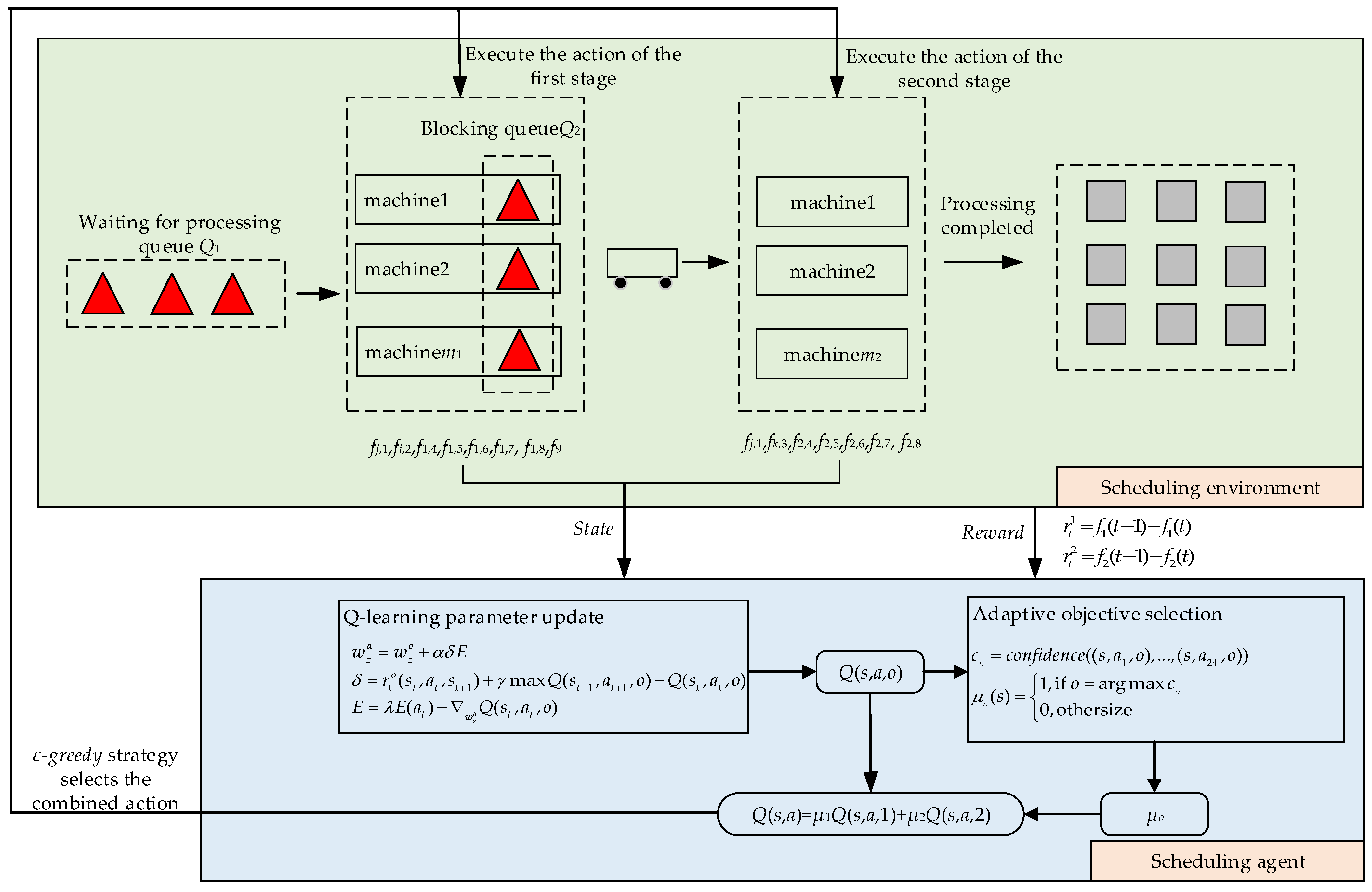
The visualization in
Figure 2 shows the specific implementation process of the algorithm. The scheduling system is in the initial state
s0 at the start of the processing time. At this point, all jobs are in the waiting processing queue
Q1, and all machines are idle. Then, an action is selected based on the
ε-greedy strategy, which involves selecting a job from queue
Q1 and an idle machine from the first stage for processing until either the set of idle machines or the set of jobs in queue
Q1 becomes empty. Following this, the blocking queue
Q2 and the set of idle machines before the second stage are evaluated. If they exist, the machine and the job are selected based on the actions. The scheduling system reaches the termination state
sT, where all processing queues are empty and all jobs have been handled, resulting in a scheduling solution.
The specific steps of the AQL algorithm are as follows:
Step 1: Initialize parameters.
Step 1.1: Input parameters of the scheduling problem: the number of jobs n, the number of machines in the first stage m1, the number of machines in the second stage m2, the processing time of each job in the two-stage machines psj, the transportation time between machines tik, the blocking power of the machine in the first stage SPi, and the transportation power of the transporter TPik.
Step 1.2: Input parameters of the Q-learning algorithm: learning rate α, discount factor γ, greedy factor ε, decay rate λ, and two m1 + m2 + n + 11 dimensional vectors E(a) = (0, 0, …, 0)T, wa = (1, 1, …, 1)T; max_episode, with the current iteration g = 1.
Step 2: Set the initial time t0 and initial state s0, and initialize two Q(s, a) tables.
Step 3: Utilize a t-test to calculate the confidence of the objective function in the current state and determine the object o where the agent has the highest confidence.
Step 4: Use the ε-greedy strategy, where we obtain a probability of ε to randomly select an action and a probability of 1 − ε to select the action with the highest Q-value from the Q-table.
Step 5: Confirm the state transition time, calculate the reward, and update the
Q-table. The reward
r(
st,
at,
st+1) is gained by taking action
at from state
st to
st+1, then updating the basis function weights
wza, hence updating the
Q-table. The update process is as follows:
Step 6: If the number of jobs that the machine processed in the second stage < n, return to Step 3; otherwise, execute Step 7.
Step 7: If the current iteration number < max_episode, g = g + 1, return to Step 2; otherwise, the algorithm is terminated.


