Use of Extended Finite Element Method to Characterize Stress Interference Caused by Nonuniform Stress Distribution during Hydraulic Fracturing

Abstract

Stress interference is the main factor affecting hydraulic fracture propagation during multi-well hydraulic fracturing; stress interference is influenced by fracture bending, fracture hits, and asymmetric fracture propagation. To investigate the role of stress interferences among hydraulic fractures with nonuniform stress distribution in an inhomogeneous formation, a hydromechanical coupling extended finite element method was adopted to investigate the fracturing paths that occurred during the first fracturing–fracturing fluid flowback–repeat fracturing process; the asymmetric fracturing that occurred at different child well locations was also studied. The results showed that the area affected by fracturing-induced stress formed a “butterfly type” area. For child wells located within the zone, stress interference resulted in asymmetric fracture propagation; meanwhile, for child wells located outside this zone, stress interference resulted in symmetric fracture geometry. The effect of stress interference on the asymmetry of child well fracture wings was found to be negatively correlated with the distance between the parent well and the child well.

1. Introduction

For low-permeability hydrocarbon reservoirs, hydraulic fracturing increases the contact area with a low-permeability matrix and improves oil and gas production efficiencies [1]. Currently, well pad hydraulic fracturing, which has parent and child wells in adjacent areas, is the main technology that is used to increase the utilization degree of reservoirs and to achieve greater economic benefits [2]. When a child well is successfully fractured, hydrocarbons can be efficiently produced in the infill area; but stress interference between adjacent hydraulic fractures is the main factor contributing to fracture bending, fracture hits, and asymmetric fracture propagation in child wells [3,4]. Therefore, it is crucial to study the parameters that affect the fracture propagation of child wells to support the production of reservoirs [5].

Normally, hydraulic fracturing procedures for parent wells are carried out prior to those for child wells; the induced stress and fluid pressure have a great effect on the magnitude and direction of the principal stresses near the fracture. For this reason, the initial stress state of adjacent child wells is considered to be a superposition of in situ stress and induced stress. During the fracturing, the overlapping initial stressed lead to the development of complex fractures near child wells. The complexity of child well fractures may cause inter-well interference, which can have a negative effect on production performance. In some cases, fracture hits induced by inter-well interference can result in abnormal pressure; this situation can further effect the cementing safety of production wells. Yaich et al. [6] have indicated that the infill fracturing of wells in the Marcellus shale reservoir caused serious interference for the production wells; the formation pressure of the fracturing wells significantly exceeded the original pressure in the work area, and there was a significant decrease in production after the fracturing at the infill wells [7]. Miller et al. [8] investigated the proportion of production wells among shale oil and gas reservoirs in the US that were affected by adjacent fracturing wells; the proportions of affected production wells was found to be as follows: 41% in Eagle Ford, 56% in Niobrara, and 64% in Woodford [9]. The research results obtained by Lindsay et al. indicated that, within a 1000 ft cluster space, 60–80% of fracturing wells can affect the productivity of adjacent production wells [10].

The asymmetric propagation of two wings along a child wellbore has been found to be the main cause of inter-well interference. Walser and Siddiqui [11] found that an asymmetric fracture could significantly reduce recoverable reserves and recovery; additionally, the properties of reservoirs, including reservoir permeability and contrasting permeability between layers, could also affect the long-term recovery of hydrocarbons [12]. Rezaei and Rafiee [13] introduced a novel approach for calculating dynamic fracture propagation and stress changes in depleted regions; they showed that, due to the asymmetry of the stress field, the fracture wing of the infilling well near the parent well changed to longitudinal; meanwhile, the other fracture wing, which was away from the parent well, remained lateral, resulting in highly asymmetric fracture geometry [14]. Based on an elegant microseismic trial conducted by the Athabasca Oil Corporation, Stephenson et al. revealed that, in a complex in situ stress field, the fracture could be asymmetric, and this fracture asymmetry is caused by the well azimuth and the state of in situ stress [15]. Hu et al. employed a 2D fracture model with microseismic observations to capture the fracture hit behavior between adjacent horizontal wells, which showed that stress barriers around horizontally fractured wells could result in asymmetric fracture wings in adjacent wells [16].

Hydraulic fracture models have been shown to be key in analyzing stress interference among hydraulic fractures. Many research efforts have been conducted in the past decade with a focus on quantitatively analyzing the interactions that occur between adjacent fractures [17,18]. Cheng et al. developed a 2D displacement discontinuous method (DDM) to investigate the impacts of the perforation cluster number and spacing on production performance; the results suggested that inadequate cluster spacing could lead to less effective or ineffective fractures, thus resulting in a lower gas rate and ultimate recovery [18,19]. Olson introduced a height-correction formula to calculate fracture morphology when multiple fractures propagate at subcritical speed; the fracture propagation velocity that occurs during stable growth is proportionate to the stress intensity factor at the fracture tips [20]. Wu et al. obtained a more accurate calculation result for multi-fracture stress interference based on the DDM by further improving Olson’s height-correction formula; the modelling results suggested that the mechanism that is key to mitigating stress–shadow effects is to maintain uniform flow resistance within each fracture [21]. Tang et al. constructed a multi-fracture propagation model based on a planar three-dimensional DDM to present complex fracture geometries in a heterogeneous stress field, and the calculation results showed that longitudinal in situ stress distribution could affect the strength of the mutual interference between fractures [22]. Zheng et al. investigated the influence of fracturing sequences on fracture propagation; fracture geometries were analyzed under different fracturing sequences [23].

From the literature review, it can be concluded that the current research mainly focused on multi-fracture propagation and the interaction mechanism between natural fractures and hydraulic fractures; fracture propagation between wells is rarely discussed. In addition, the DDM, FEM, and DEM were the main methods of exploring fracture propagation in numerical simulations. In these simulations, the hydraulic fracture propagation trajectory was predetermined, and it cannot consider the effect of the stress field change on fracture propagation. Comparatively, the XFEM can simulate the effect of the stress field change on fracture propagation; thus, the XFEM was selected for the present study. In this work, we present a numerical investigation of fracture propagation for fractured parent wells and child wells in the Junggar Basin. The first challenge is to describe the inhomogeneous distribution of geostress; then, we must capture the fracture bending process with a consideration of the anisotropic characteristics of the reservoir. Here, we determine the rock parameters using logging data (Section 2.1 and Section 2.2) and estimate the magnitude and direction of 3D principal stresses through inversion analysis based on geostress field test data (Section 2.3 and Section 2.4). Then, we adopted a hydro-mechanical coupling extended finite element method (XFEM) to investigate the fracturing paths of the parent well and the child well, and the relevant parameters that affect the asymmetry of child well fractures are discussed (Section 3).

2. Methods

2.1. Rock Mechanical Tests

In this work, nineteen core samples were collected from the parent well in a sand–mudstone interlayered reservoir in the Junggar Basin for a rock mechanic test. Cylinders with a diameter of 25 mm and a length of about 50 mm were prepared. In the experiment, the loading speed of the samples was 0.005 mm/min, and the samples were cut from a drill core. For the uniaxial test, the cylinders were placed in the loading cell; then, the axial load increased at a constant rate. The stress–strain curves were recorded along this process. The test results on the 10 rock samples are shown in

Table 1. Test results of the 10 rock samples.

Sample ID	Depth (m)	Density (g/cm3)	Porosity (%)	Confining Pressure (MPa)	Compressive Strength (MPa)	Poisson’s Ratio (1)	Es (MPa)
1-1	645.35	2.59	1.5	0.0	62.544	0.306	54,760
1-2	645.38	2.60	1.1	0.0	53.202	0.057	10,544
1-3	645.67	2.63	1.2	3.0	92.200	0.266	47,382
1-4	645.72	2.61	1.8	6.0	118.385	0.218	40,955
1-5	645.87	2.64	1.4	3.0	89.452	0.215	37,995
1-6	645.83	2.64	1.8	9.0	107.814	0.241	37,939
1-7	646.02	2.63	1.1	6.0	108.887	0.217	38,042
1-10	646.54	2.62	1.3	9.0	81.300	0.195	28,079

.

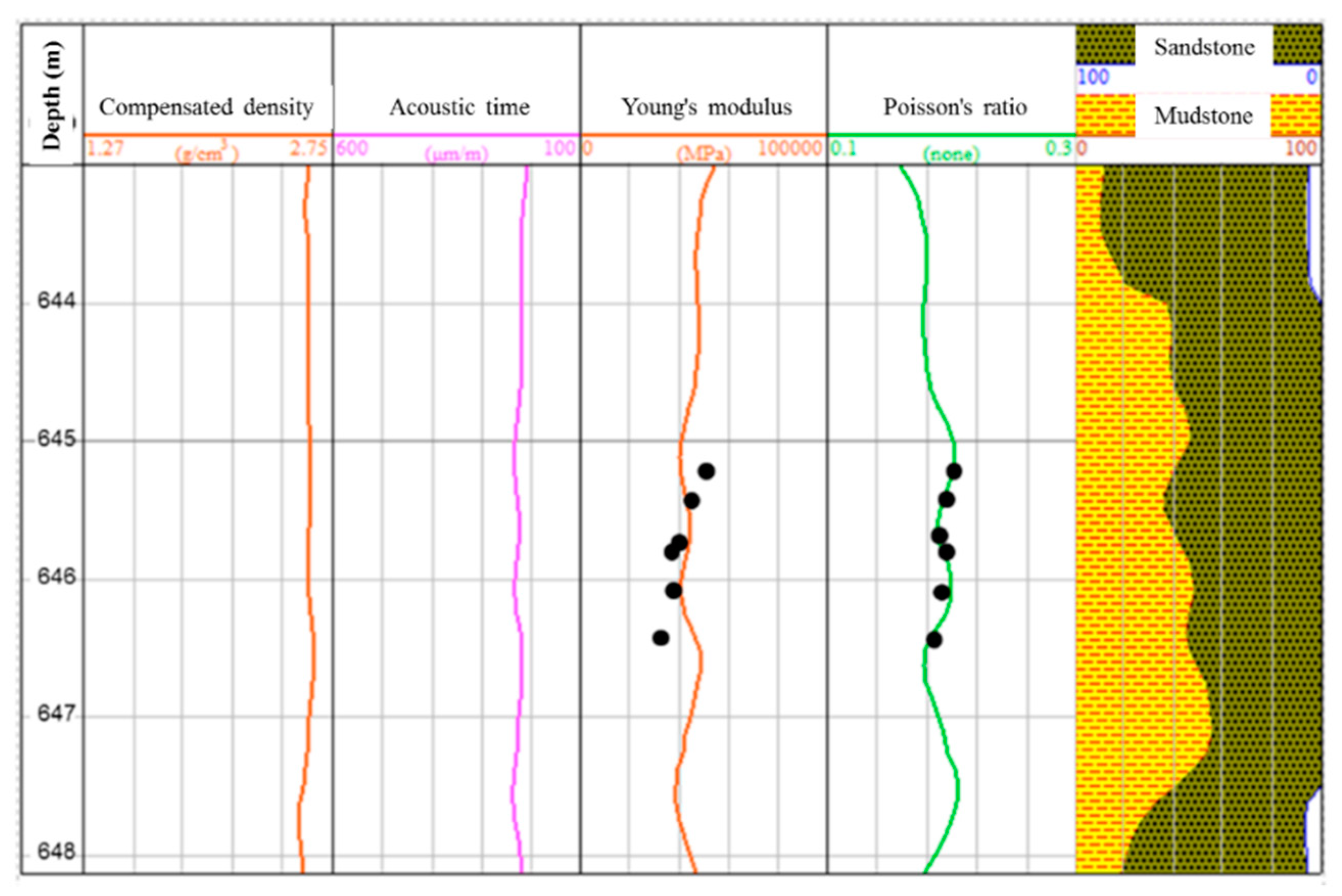
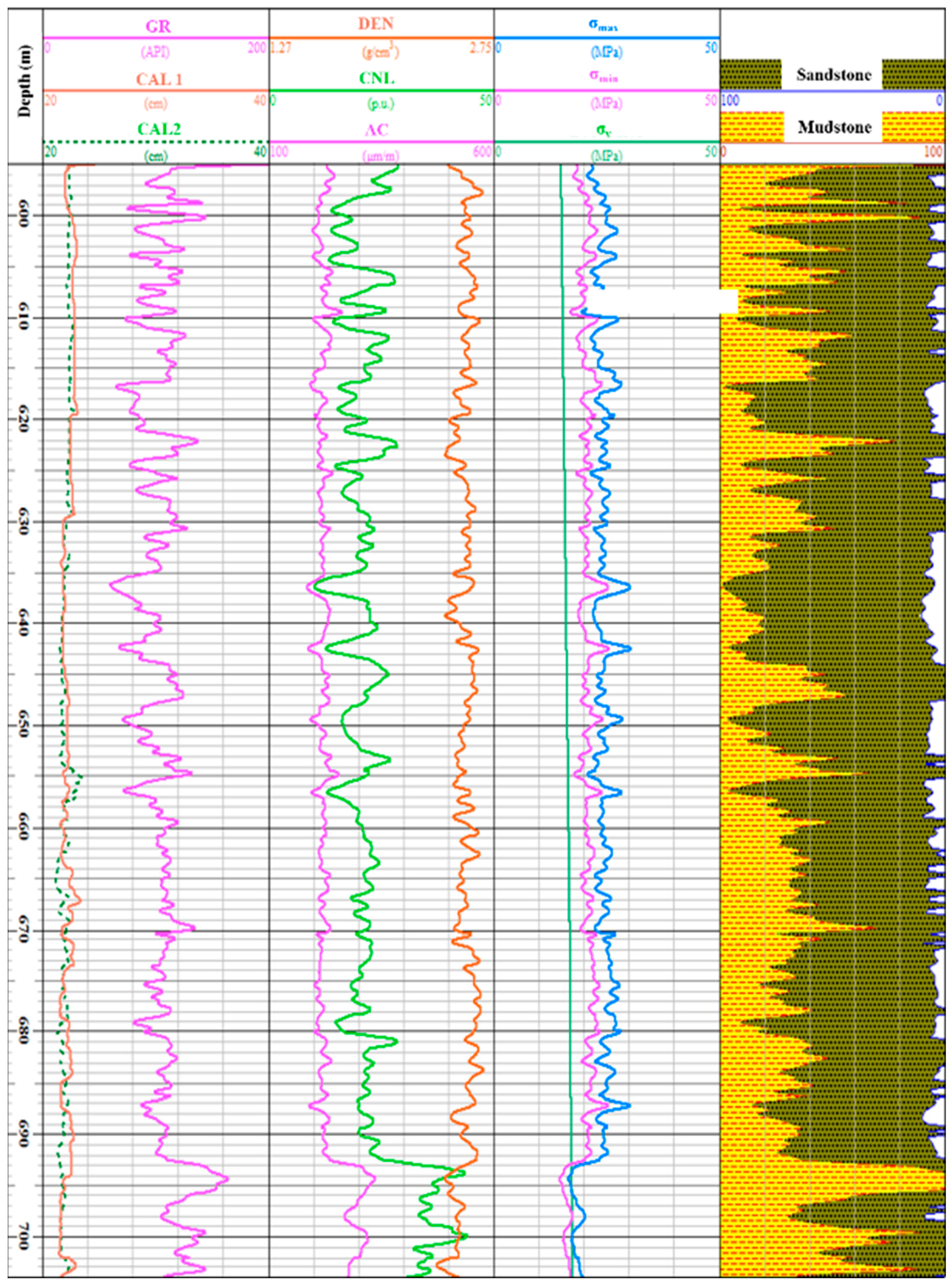
2.2. Determining Rock Parameters with Logging Data

In order to continuously estimate the rock mechanical parameters, the dynamic Young’s modulus (Ed) and dynamic Poisson’s ratio (ν_d) were calculated using acoustic logging data by Empirical Correlations (1) and (2):

$$E_d={\displaystyle \frac{DEN}{{DTS}^2}}\left({\displaystyle \frac{3{DTS}^2-4{AC}^2}{{DTS}^2-4{AC}^2}}\right)$$

(1)

$${\mu }_d={\displaystyle \frac{{DTS}^2-2{AC}^2}{2({DTS}^2-4{AC}^2)}}$$

(2)

By fitting dynamic rock mechanical parameters to the static rock mechanical parameters, the conversion relations can be presented as follows:

$$E_s=1.1572E_d-6038.3$$

(3)

$${\mu }_s=1.8506{E\mu }_d-0.2502$$

(4)

$$UCS=45.3\mathrm{e}\mathrm{x}\mathrm{p}\left(0.0196E_s\right)$$

(5)

$$ST=6169.32{({∆t}_s/{\rho }_b)}^{-1.422}$$

(6)

In order to verify the usability of the transformation models in Figure 1, we compared the core test results with the rock mechanical curves determined by Equations (3) and (4). Based on these models and the logging data of the parent well, the curves of Young’s modulus and Poisson’s ratio at a depth of 643–645 m are presented in Figure 1; the core test results at the same depth (the black dots) present a good correlation with the curves. This is an indication of the accuracy of these transformation models. We applied these models to the entire well section of the parent well. Figure 2 shows the rock mechanic parameter curves in the depth range of 940–1030 m.

2.3. Estimation of the Pore Pressure

In view of the low mud content of the sand–mudstone alternate formation, we adopt an equivalent depth method to carry out the prediction of pore pressure. For rocks of different depths but with the same physical properties, the equivalent depth method assumes that the effective stress on the rock skeleton is equal [5]:

$${(\mathsf{\sigma }-{\alpha }_p{p}_p)}_1={(\mathsf{\sigma }-{\alpha }_p{p}_p)}_2$$

(7)

The primary premise of using the equivalent depth method is to predict formation pressure based on logging data; accordingly, one can establish an accurate mudstone normal compaction trend equation. Therefore, according to the logging data, the normal compaction trend equations of the sand and mudstone formations in the study area were established, respectively. Based on the established normal compaction trend line, if the abnormal pressure segment had the same acoustic time difference as a point on the normal compaction trend line, then the two points are indicated to have the same degree of compaction. The pore pressure of the target layer can be calculated as follows:

$$P_A={\rho }_r^{A}g{h}_A-\mathrm{g}({\rho }_r^N-{\rho }_w^N)h_N$$

(8)

where $h_A$ and $h_N$ are the depth of the target layer and the equivalent depth point, ${\rho }_r^A$ and ${\rho }_r^N$ are therock density, and ${\rho }_w^N$ is the average pore fluid density.

2.4. Estimation of the Principal Stresses

The in situ geostress at the perforation was obtained by a hydraulic fracturing test. According to the principle of the lowest energy, a hydraulic fracture is always initiated and propagated along the direction that is perpendicular to the minimum principal stress (${\sigma }_{min}$); thus, the fracture indicates the direction of the maximum horizontal principal stress (${\sigma }_{max}$). The closing pressure of the fracture can be used as an indicator for the magnitude of the horizontal minimum principal stress; the horizontal maximum principal stress could be further calculated from the breaking pressure. Under fully elastic conditions, when drilling the borehole parallel to a certain principal stress direction, the circumferential stress (${\sigma }_{\theta }$) and the normal stress (${\sigma }_r$) near the wellbore could be presented as follows:

$${\sigma }_{\theta }={\displaystyle \frac{1}{2}}\left({\sigma }_{max}+{\sigma }_{min}\right)\left(1+{\displaystyle \frac{r_a^2}{r_i^2}}\right)+{\displaystyle \frac{1}{2}}\left({\sigma }_{max}-{\sigma }_{min}\right)\left(1+3{\displaystyle \frac{r_a^4}{r_i^4}}\right)cos2\theta -P_w{\displaystyle \frac{r_a^2}{r_i^2}}$$

(9)

$${\sigma }_r={\displaystyle \frac{1}{2}}\left({\sigma }_{max}+{\sigma }_{min}\right)\left(1+{\displaystyle \frac{r_a^2}{r_i^2}}\right)+{\displaystyle \frac{1}{2}}\left({\sigma }_{max}-{\sigma }_{min}\right)\left(1-4{\displaystyle \frac{r_a^4}{r_i^4}}+3{\displaystyle \frac{r_a^4}{r_i^4}}\right)cos\theta +P_w{\displaystyle \frac{r_a^2}{r_i^2}}$$

(10)

where $r_a$ is the wellbore radius, $r_i$ is the radial distance from the wellbore center, and $P_w$ is the fluid pressure in the wellbore. The shear stress could be presented as follows:

$${\tau }_{r\theta }=-{\displaystyle \frac{1}{2}}\left({\sigma }_{max}-{\sigma }_{min}\right)\left(1+2{\displaystyle \frac{r_a^2}{r_i^2}}-3{\displaystyle \frac{r_a^4}{r_i^4}}\right)sin2\theta$$

(11)

On the wellbore wall, when →$r_a$ and $\theta$ = 0:

$${\sigma }_{\theta }=3{\sigma }_{min}-{\sigma }_{max}-P_w$$

(12)

$${\sigma }_{min}=P_{so}+\rho h-P_m-P_b$$

(13)

$${\sigma }_{max}={\sigma }_{min}+4(P_e-P_{so})$$

(14)

$${\sigma }_v=g{\sum }_{i=1}^n{\rho }_i{∆D}_i$$

(15)

where $P_m$ is the friction loss along the well section, $P_b$ is the formation pore pressure, $P_e$ is the fracture extension pressure, and $P_{so}$ is the instantaneous shut-in pressure. $P_m$, $P_b$, $P_e$, and $P_{so}$ are from the field fracturing data; the stress state at the perforation can be calculated by Equations (13)–(15). To estimate the principal stresses along the well continuously, here, we adopt the combined spring model. This model assumes that the rock is a homogeneous and isotropic linear elastic body without relative displacement during tectonic movements; the horizontal strain keeps constant. With these assumptions, the combined spring model could comprehensively consider the influence of formation rock mechanics, pore pressure, and tectonic action on principal stresses. Each principal stress component could be presented as follows:

$${\sigma }_{max}=({\displaystyle \frac{\mu }{1-\mu }}+{\beta }_1)({\sigma }_v-{\alpha P}_p)+{\alpha P}_w$$

(16)

$${\sigma }_{min}=({\displaystyle \frac{\mu }{1-\mu }}+{\beta }_2)({\sigma }_v-{\alpha P}_p)+{\alpha P}_w$$

(17)

The tectonic stress coefficients ${\beta }_1$ and ${\beta }_2$ can be determined by the stress state at the perforation; thus, the geostress along the wellbore can be obtained by Equations (16) and (17). The principal stresses along parent well L25 are shown in Figure 3.

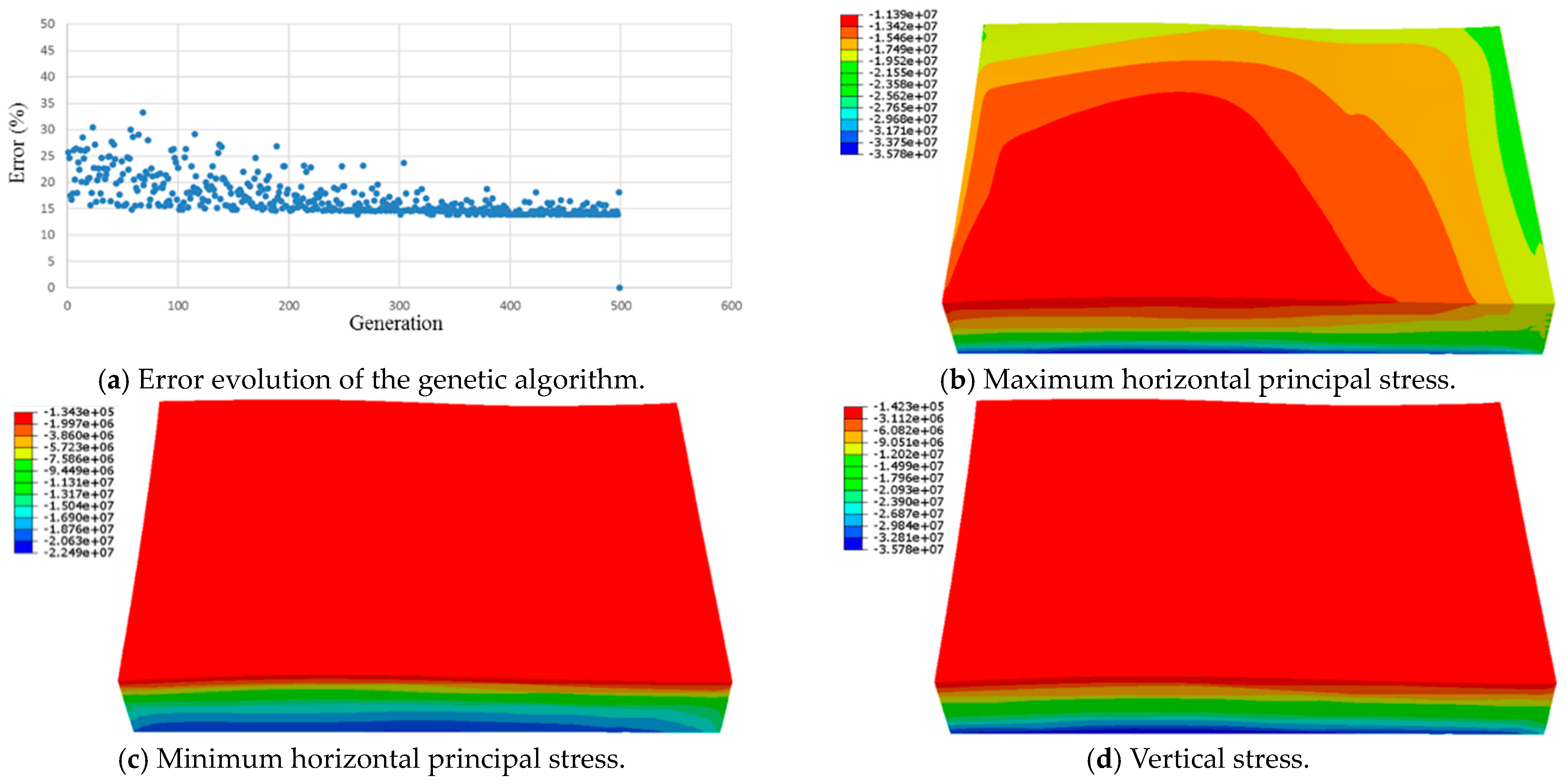
2.5. Three-Dimensional Geostress Field

In situ stress forms under the combined influences of the weight of the rock mass and the tectonic movement, as well as the physicochemical changes in the geological mass, topography, and temperature stress. The geostress field test that was conducted during the operation was the most direct approach for studying deep geostress; however, the cost of in situ stress testing was high, the shapes of the deep geological structures were complex, the distribution of the formation media was uneven and discontinuous, and the rock physical and mechanical properties were variable. The test results only presented the stress conditions in the area near the test point. Therefore, a feasible method was to construct a reasonable geomechanical model on the basis of a fine analysis of the geological structures, and to perform a numerical simulation inversion analysis based on the in situ stress data of limited test points and mathematical and mechanical theories; this approach enabled us to further quantitatively study the stress field in a deep area and analyze the horizontal distribution of the stress field in the deep area.

Taking the tested in situ stress as a basic constraint, the inversion analysis of the 3D geostress could be accomplished by determining the boundary load of the calculation model. The far-field tectonic stress state could be considered as the superposition of the following two basic tectonic states: (a) horizontal extrusion or stretching along the X and Y directions and (b) uniform shear structure deformation. Thus, the displacement boundaries in the model can be expressed as follows:

$$\left\{\begin{array}{c}{u}_x=P_{xn}+P_{t1}\\ u_y=P_{yn}+P_{t2}\end{array}\right.$$

(18)

where $u_x$ and $u_y$ are the horizontal loading vectors in the X and Y directions; $P_{xn}$ and $P_{yn}$ are the horizontal extrusion or tensile vectors; $P_{t1}$ and $P_{t2}$ are the horizontal shearing vectors.

The initial stress field inversion was based on an iterative algorithm that gradually corrects the trial calculation of parameters until the error function tended to a minimum. The geostress component can be noted as follows:

$${\sigma }_{ij}=f\left(P_{xn},P_{yn},P_{t1}{P}_{t2}\right)$$

(19)

The field geostress component was noted as ${\sigma }_{ij}^{mk}$; at the same spot, the geostress component calculated by the finite element model was ${\sigma }_{ij}^{ck}$. The error function, $\psi$, can be expressed using the deviation of the calculated stress from the measured stress:

$$\psi \left(P_{xn},P_{yn},P_{t1},P_{t2}\right)=\left|\left.{\sigma }_{ij}^{ck}-{\sigma }_{ij}^{mk}\right|\right./{\sigma }_{ij}^{ck}$$

(20)

In this work, numerical inversion was accomplished by a genetic algorithm in MatLab, 2020. The boundary vectors $P_{xn},P_{yn},P_{t1},\mathrm{a}\mathrm{n}\mathrm{d}{P}_{t2}$ are noted as input parameters, and the geostress components, ${\sigma }_{ij}$, calculated by the finite element method, are noted as output parameters. The initial error decreased gradually with the genetic generation (Figure 4a); after the inheritance was conducted to the 500th generation, the inversion accuracy rate reached 93.3%. The inversed 3D principal stress fields of an 8.0 × 5.0 km² area at a depth of 100–1200 m are presented in Figure 4b–d.

The rock mechanical properties and stress fields, calculated according to the experimental tests and logging calculations, are depicted in

Table 2. Parameters of the hydraulic fracturing simulation.

Item	Parameters	Unit	Value
Rock Mechanical properties	Young’s Modulus	GPa	27.6
	Poisson’s Rate	Dimensionless	0.34
	Tensile strength	MPa	8.42
	Shear strength	MPa	8.61
	Permeability	mD	0.35
Injection Parameters	Injection rate	m3/min	2.0
	Viscosity of fracturing fluid	mPa.s	20.0
Stress Field	Vertical stress	MPa	15.0
	Maximum horizontal principal stress	MPa	13.6
	Minimum horizontal principal stress	MPa	11.7

.

3. Hydraulic Fracture Modelling

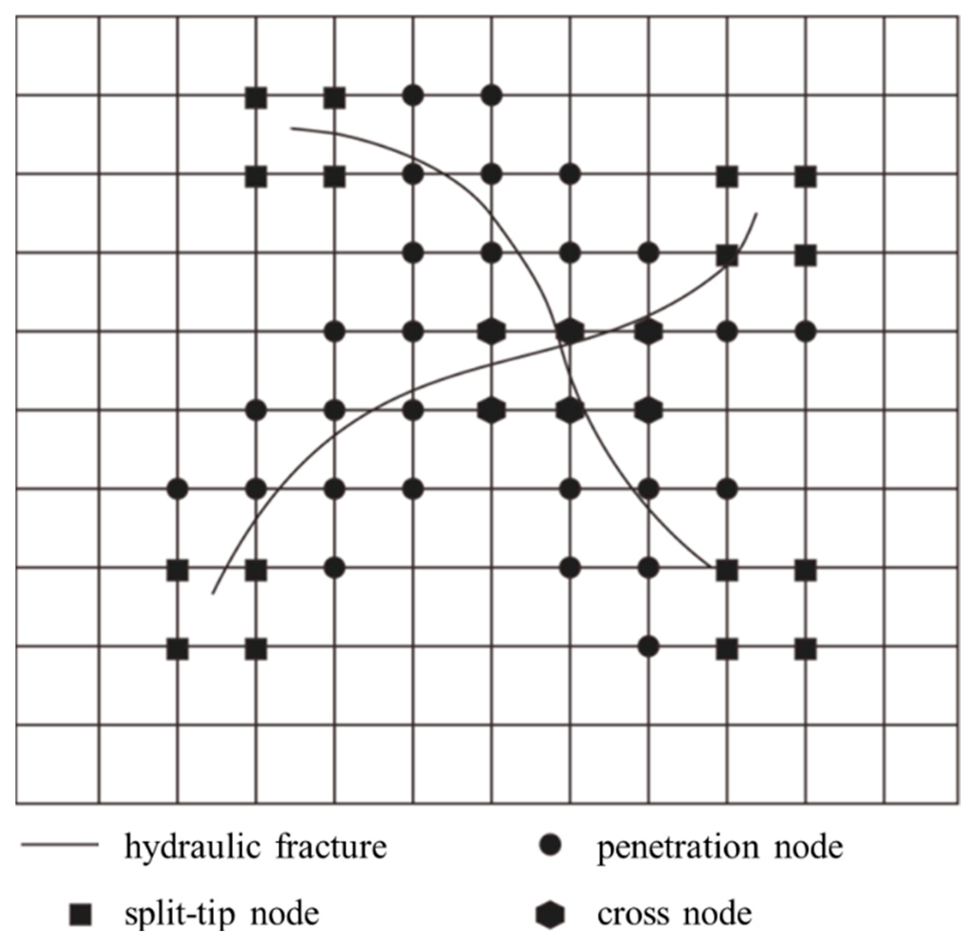
3.1. Modelling Approach

The extended finite element method (XFEM) uses the level set method or the fast advance method to introduce the modification of the shape function within the unit. The continuous function was used to characterize the continuous region, and the enhanced function was used to represent the non-continuous region. The introduced enhancement functions mainly include three functions: the Heaviside function to characterize the discontinuity of the displacement field, the Junction function to characterize the fracture crossing, and the fracture tip increase function to characterize the fracture tip singularity field. The corresponding unit types are the penetration node, the cross node, and the split-tip node (Figure 5).

The approximate form of displacement $\mathrm{u}\left(\mathrm{r}\right)$ at any point in the finite element model with cracks is as follows:

$$\begin{gathered} \mathrm{u}\left(\mathrm{r}\right)=\sum _{i\in M_{\mathrm{r}}}{N}_{\alpha \left(i\right)}\left(\mathrm{r}\right)u_i+\sum _{j\in M_{\mathrm{r}}}{N}_{\alpha \left(j\right)}\left(\mathrm{r}\right){\left(H\left(\mathrm{r}\right)-H\left({\mathrm{r}}_j\right)\right)\mathrm{a}}_j \\ +\sum _{h\in M_{\mathrm{r}}}{N}_{\alpha \left(h\right)}\left(\mathrm{r}\right){\left(J\left(\mathrm{r}\right)-J\left({\mathrm{r}}_h\right)\right)b}_h+\sum _{k\in M_{\mathrm{r}}}{N}_{\alpha \left(k\right)}\left(\mathrm{r}\right)\left[\sum _{i=1}^4\left(F_l\left(\mathrm{r}\right)-F_l\left({\mathrm{r}}_k\right)\right)c_k^l\right] \end{gathered}$$

(21)

where r is the position vector; $M_{\mathrm{r}}$, $M_{{\mathrm{r}}_j}$, $M_{{\mathrm{r}}_h}$, and $M_{{\mathrm{r}}_k}$ are the ordinary node set, step function enhanced node set, connection function node set, and fracture tip enhanced node set of the unit where r is located; ${\mathrm{u}}_i$ is the node displacement; ${\left\{N_{\alpha }\right\}}_{\alpha =1}^4$ is a shape function; $\alpha \left(i\right)$ is the mapping function from global coordinates to local coordinates;$H\left(\mathrm{r}\right)$, $J\left(\mathrm{r}\right)$, and $F_l\left(\mathrm{r}\right)$ are the Heaviside function value, the Junction function value, and the fracture tip enhancement function value of Gaussian point x, respectively. ${\mathrm{a}}_j$, $b_h$, and $c_k^l$ are the enhanced node degrees of freedom vectors for the penetrating element, the intersection element, and the fracture tip element, respectively. The Heaviside function is a step function using level set function to determine whether a point is located on the upper or lower surface of the crack, thereby indicating the discontinuity of the displacement field:

$$H\left(\mathrm{r}\right)=\mathrm{s}\mathrm{g}\mathrm{n}\left(f\right(\mathrm{r}\left)\right)$$

(22)

where the level set function $f\left(\mathrm{r}\right)$ = 0 represents the fracture surface. If point r was closest to point r* on the fracture surface, the normal vector at point r* was ${\mathrm{e}}_n$, and when ${\mathrm{e}}_n·\left(\mathrm{r}-{\mathrm{r}}^{*}\right)>$0 and $f\left(\mathrm{r}\right)>0$, point r was located above the fracture surface. The Junction function was a connection function that reflects the effect of the intersection of cracks:

$$J\left(\mathrm{r}\right)=\left\{\begin{array}{c}sgn\left(f_2\left(\mathrm{r}\right)\right)-sgn\left(f_2\left({\mathrm{r}}_h\right)\right)f_2\left(\mathrm{r}\right)·f_2\left({\mathrm{r}}_0\right)>0\\ sgn\left(f_1\left(\mathrm{r}\right)\right)-sgn\left(f_1\left({\mathrm{r}}_h\right)\right)f_2\left(\mathrm{r}\right)·f_2\left({\mathrm{r}}_0\right)<0\end{array}\right.$$

(23)

where sgn (r) is the sign function; $f_1\left(\mathrm{r}\right)$ is the level set function of hydraulic fractures; $f_2\left(\mathrm{r}\right)$ is the level set function of natural fractures. The fracture enhancement function is to extract the function reflecting the singularity of the fracture tip according to the progressive displacement field of the fracture tip in linear elastic fracture mechanics, namely:

$${\left\{F\left(r,\mathsf{\phi }\right)\right\}}_{l=1}^4=\sqrt{r}\left\{\mathrm{s}\mathrm{i}\mathrm{n}\left(\phi /2\right),\mathrm{c}\mathrm{o}\mathrm{s}\left(\phi /2\right),\mathrm{s}\mathrm{i}\mathrm{n}\left(\phi /2\right)\mathrm{s}\mathrm{i}\mathrm{n}\left(\phi \right),\mathrm{c}\mathrm{o}\mathrm{s}\left(\phi /2\right)\mathrm{s}\mathrm{i}\mathrm{n}\left(\phi \right)\right\}$$

(24)

where (r,$\mathsf{\phi }$) represents the polar coordinates of the local coordinate system centered on the fracture tip.

3.2. Hydraulic Fracture Modelling at the Parent Well

The targeted reservoir was at a depth of 620 m; the material parameters are calculated by Equations (3)–(6) with logging data. Based on Saint-Venant’s principle, the 3D geostress field near the wellbore was abstracted from the inversed principal stress field in Figure 6a and shown in Figure 6c. The hydraulic fractures extend in a perpendicular direction from the maximum principal stress ${\sigma }_v$, and form a vertical fracture in the target reservoir. In the horizontal direction, the range of the model was 1000 m × 1000 m (Figure 6d). According to the fracturing design at parent well L25 provided by the industry, the fracture operation included four stages, and the time was close to the real time.

• Stage 1: The first fracturing occurred at 50 min; the flow ratio of the fracturing fluid was 2 m³/min.
• Stage 2: Fracturing fluid flowback occurred for 360 min.
• Stage 3: Fracturing repeated for 50 min; the flow ratio of the fracturing fluid was 2 m³/min.

After the fracturing operation at the parent well, the industry planned to place a child well at candidate location (Figure 6c). The fracturing operation at the child well occurred at 100 min; the flow ratio of the fracturing fluid was 2 m³/min.

3.2.1. First Fracturing Modelling

The evolution of fluid pressure at the perforation with time is presented in Figure 7. The extrusion stage was not included in this work; at the beginning of the fracturing process, the fluid pressure at the perforation point rises sharply until a breaking pressure is reached. Then, the fluid pressure drops rapidly; following this, it basically maintains a stable value during the subsequent fracture propagation process. The accuracy of the numerical model was verified indirectly using field fracturing data of the parent well. The field fracture pressure was 19.30 MPa and the closing pressure was 14.73 MPa. In our modeling results, the simulated fracture pressure was 18.13 MPa and the closure pressure was 12.33 MPa; the agreement between the simulation results and the field fracturing data was 87.32%, indicating the feasibility of the proposed approach.

At the beginning of the fracturing process, a fracture propagates in the direction of the perforation. After the fracture length reaches about 10 times the length of the borehole’s diameter, it propagates along the direction of the maximum principal stress, and thus forms a turning fracture. The induced stress was tensile at the fracture tip; in the normal direction of the fracture length, it was compressive. This induced compressive stress changes the stress state near the fracture; the direction of ${\sigma }_{max}$ changed from NNW–SSE to E–W (Figure 7b). The direction of the minimum horizontal principal stress before and after the initial fracturing changes accordingly (Figure 7d). However, the direction of the horizontal principal stress near the fracture tip was not significantly affected; for this reason, the propagation direction of the fracture was not affected by the induced stress.

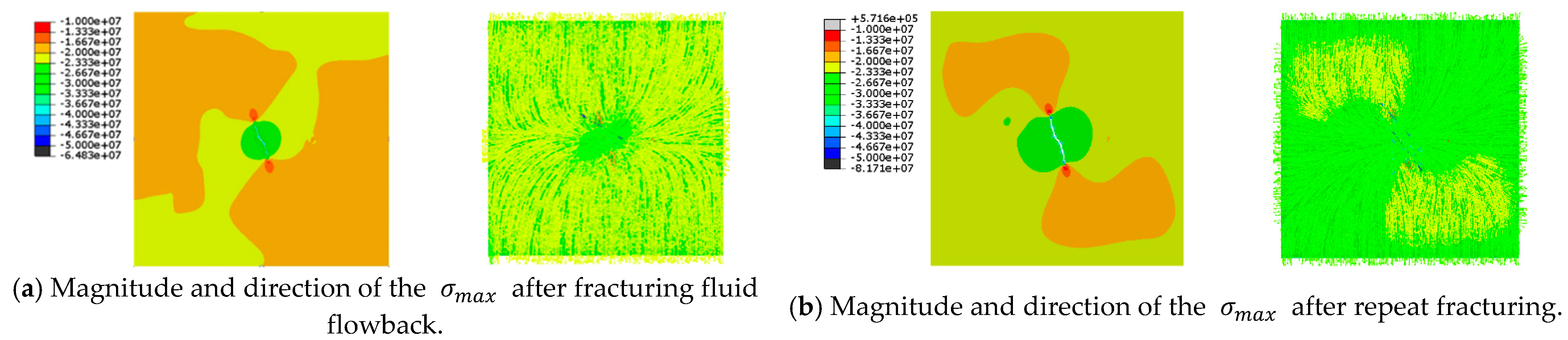
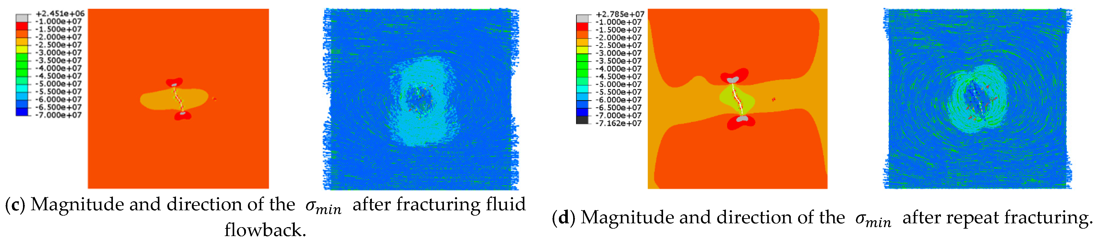
3.2.2. Fracturing Fluid Flowback and Repeat Fracturing

After the fracturing fluid flowback for 360 min, the pore pressure near the fracture dropped by about 3~5 MPa; the magnitudes of ${\sigma }_{max}$ and ${\sigma }_{min}$ changed accordingly, but their directions were not affected. The fracture morphology did not change significantly during the flowback process (Figure 8a,c). Then, during the repeated fracturing process at well L25, the fracture width gradually increased in the first 20 min, but the fracture length did not change significantly. After 30 min, the fracture continued to propagate along the direction of the maximum principal stress; this range is influenced by fracturing-induced stress, which further expands here (Figure 8b,d).

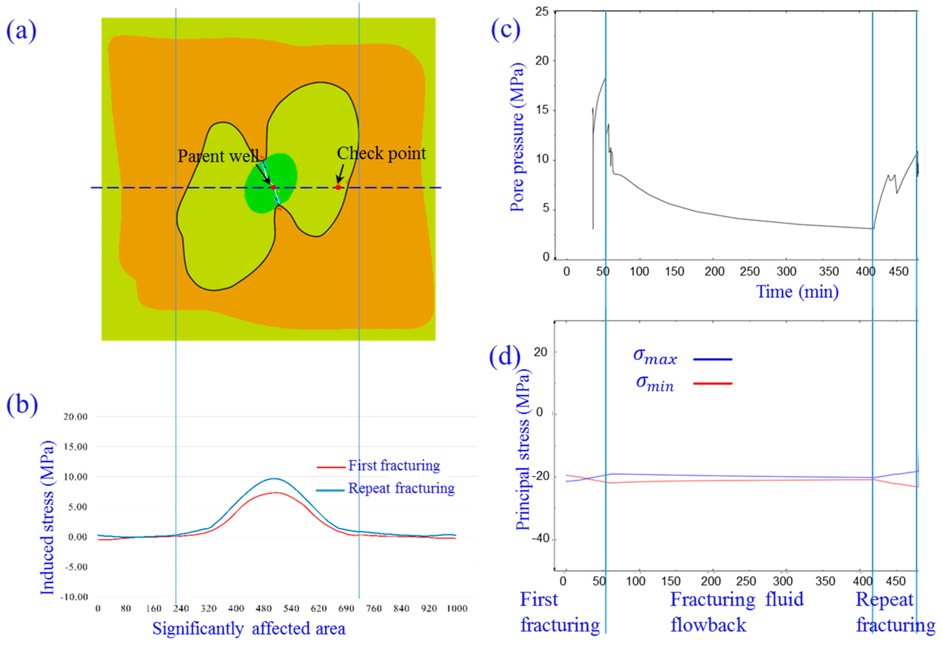
3.3. Modelling Result Discussion

After the first fracturing process, due to the induced tensile stress at the fracture tips and the induced compressive stress in the normal direction of the fracture length, the area affected by fracturing-induced stress forma a “butterfly type” area (shown in Figure 9a). In the E–W direction, the range affected after the first fracturing was 1.5–2 times the length of the fracture. After repeated fracturing, the magnitude of the induced stress was increased, but its influence range did not change significantly (Figure 9b). The fluid pressure variation at the parent well was present in Figure 9c; as shown here, the fluid pressure rose rapidly during the first fracturing process, until it reached the breaking pressure; then, it decreased throughout the fracturing fluid flowback process. Afterward, the repeat fracturing enhanced the fluid pressure again. Here, we investigate the variation in principal stresses at the checkpoint during parent well fracturing. The checkpoint is located 200 m east from the parent well; this is inside the “butterfly type” affected area that is shown in Figure 9a. As shown in Figure 9d, the maximum principal stress turned into the minimum principal stress after the first fracturing process; the repeated fracturing led to an increase in the difference between the maximum and minimum principal stresses; the reorientation of the stresses has a significant impact on the fracturing of the child well here. As indicated in Figure 9a, the checkpoint was the point at which the geostress and the pore pressure were measured during the fracturing of the parent well.

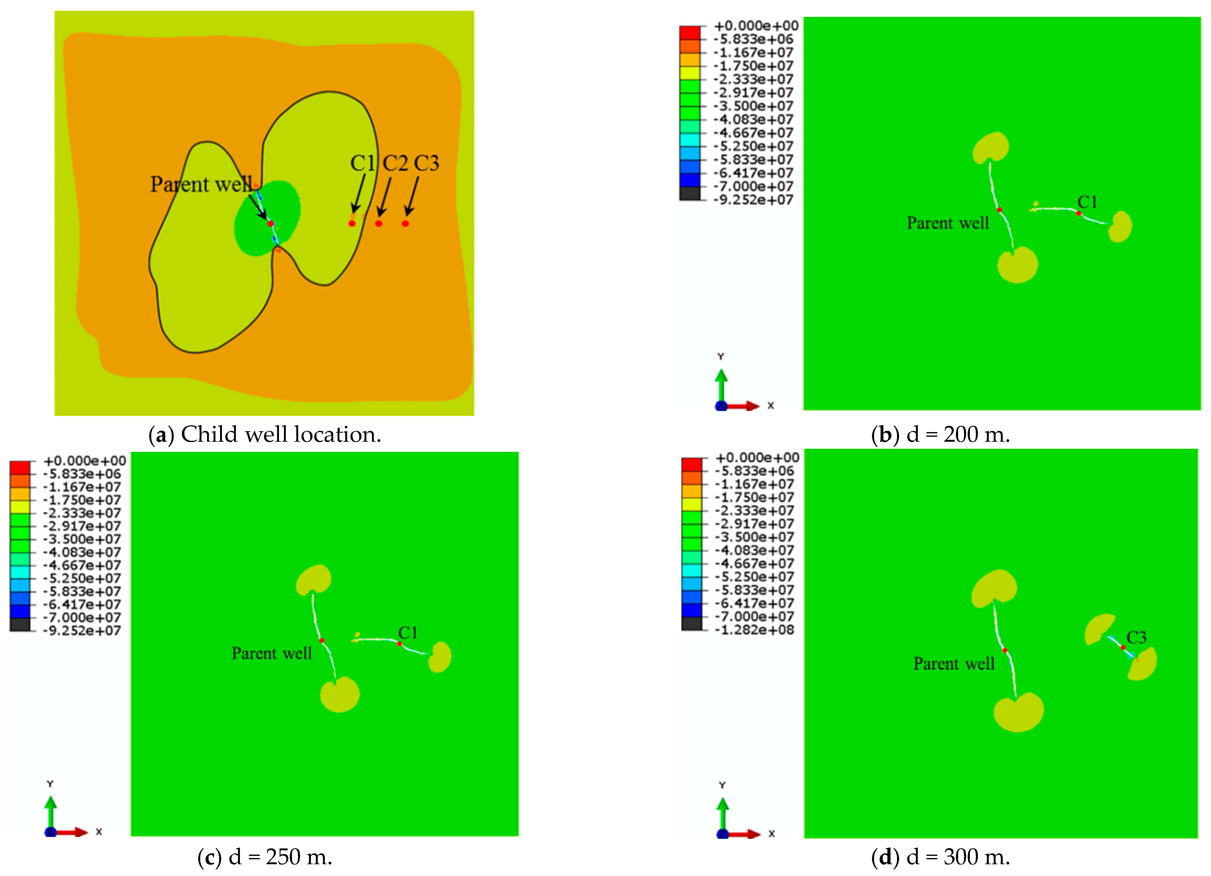
3.4. Fracturing of the Child Well

In the candidate child well location, the induced stress field was superimposed onto the in situ stress field; this stress state change can significantly impact the fracturing of the child well. Here, we present several child wells in different locations to illustrate how inter-well interference affects the fracture wings of the child well. After the parent well repeatedly fractured, a child well fracturing was conducted for d = 200 m, d = 250 m, and d = 300 m, where d represents the distance from the child well to the parent well on the E–W direction. Figure 10 presents the fracture geometry after fracturing at the child well for 100 min, with a flow ratio of 2 m³/min; the fracture width (white curve) was magnified 50 times for visualization. Child well C1 is located within the “butterfly type” zone in Figure 9a, while child wells C2 and C3 are located outside this zone. As shown in Figure 10b, the left fracture wing of the child well propagates in the east–west direction, which is significantly affected by the compressive stress induced by parent well fracturing; meanwhile, the right wing propagates in the northwest–southeast direction and thus present asymmetric fracture propagation. When the child well is located outside the “butterfly type” zone, Figure 10c,d present the symmetric fracture geometry. The effect of stress interference on the asymmetry of child well fracture wings was negatively correlated with d.

4. Conclusions

In this study, we investigated stress interference among hydraulic fractures with nonuniform stress distribution in an inhomogeneous reservoir. We determined the rock parameters with rock mechanical tests and field logging data, and then estimated the magnitude and direction of 3D principal stresses by inversion analysis; this analysis was based on geostress field test data. The hydromechanical coupling XFEM was adopted to investigate the fracturing paths for the fracture wings of the parent well and the child well, and the hydraulic fracturing at different child well locations were also studied. The conclusions can be summarized as follows:

(1)

Due to the induced tensile stress at the fracture tips and the induced compressive stress in the normal direction of the fracture length, the area affected by fracturing-induced stress formed a “butterfly type” area. In the E–W direction, the affected range after the first fracturing process at the parent well was 1.5–2 times the fracture length.

(2)

The fracturing fluid flowback at the parent well changed the magnitude of the maximum and minimum horizontal principal stresses, but their directions were not affected. After repeated fracturing at the parent well, the magnitude of the fracturing-induced stress increased, but its influence range did not increase significantly.

(3)

For a child well located within the “butterfly type” zone, the stress interference results in an asymmetric fracture propagation; meanwhile, for a child well located outside of this zone, a symmetric fracture geometry occurs.

(4)

The non-concurrent parent well and child well completions are the main cause of stress interference, and the effect of stress interference on the asymmetry of the child well fracture wings was negatively correlated with the distance between the parent well and the child well.

(5)

The fracture geometry under different well spacings was analyzed; this provided a method of optimizing the well space during parent well fracturing. In the simulations, the formation properties were assumed to be uniform. This was necessary for investigating the impact of nonuniform stress distribution on fracture propagation.

References

1. Bowers, G.L. Pore pressure estimation from velocity data: Accounting for overpressure mechanisms besides undercompaction. SPE Drill. Complet. 1995, 10, 89–95. [Google Scholar] [CrossRef]
2. Cheng, Y. Impacts of the number of perforation clusters and cluster spacing on production performance of horizontal shale-gas wells. SPE Reserv. Eval. Eng. 2012, 15, 31–40. [Google Scholar] [CrossRef]
3. Esquivel, R.; Blasingame, T.A. Optimizing the Development of the Haynesville Shale-Lessons-Learned from Well-to-Well Hydraulic Fracture Interference. In Proceedings of the Unconventional Resources Technology Conference, Austin, TX, USA, 24–26 July 2017; Society of Exploration Geophysicists, American Association of Petroleum: Houston, TX, USA, 2017; pp. 1005–1026. [Google Scholar]
4. Gala, D.P.; Manchanda, R.; Sharma, M.M. Modeling of fluid injection in depleted parent wells to minimize damage due to frac-hits. In Proceedings of the Unconventional Resources Technology Conference, Houston, TX, USA, 23–25 July 2018; Society of Exploration Geophysicists, American Association of Petroleum: Houston, TX, USA, 2018; pp. 4118–4131. [Google Scholar]
5. Guo, X.; Ma, J.; Wang, S.; Zhu, T.; Jin, Y. Modeling Interwell Interference: A Study of the Effects of Parent Well Depletion on Asymmetric Fracture Propagation in Child Wells. In Proceedings of the SPE/IATMI Asia Pacific Oil & Gas Conference and Exhibition, Bali, Indonesia, 29–31 October 2019. [Google Scholar]
6. Hu, X.; Liu, G.; Luo, G.; Ehlig-Economides, C. Model for Asymmetric Hydraulic Fractures with Nonuniform-Stress Distribution. SPE Prod. Oper. 2019, 36, 1–11. [Google Scholar] [CrossRef]
7. Lawal, H.; Jackson, G.; Abolo, N.; Flores, C. A novel approach to modeling and forecasting frac hits in shale gas wells. In Proceedings of the EAGE Annual Conference & Exhibition Incorporating SPE Europec, London, UK, 10–13 June 2013; Society of Petroleum Engineers: Richardson, TX, USA, 2013. [Google Scholar]
8. Lindsay, G.; Miller, G.; Xu, T.; Shan, D.; Baihly, J. Production performance of infill horizontal wells vs. pre-existing wells in the major US unconventional basins. In Proceedings of the SPE Hydraulic Fracturing Technology Conference and Exhibition, The Woodlands, TX, USA, 23–25 January 2018; Society of Petroleum Engineers: Richardson, TX, USA, 2018. [Google Scholar]
9. Miller, G.; Lindsay, G.; Baihly, J.; Xu, T. Parent well refracturing: Economic safety nets in an uneconomic market. In Proceedings of the SPE Low Perm Symposium, Denver, CO, USA, 5–6 May 2016; Society of Petroleum Engineers: Richardson, TX, USA, 2016. [Google Scholar]
10. Moës, N.; Belytschko, T. Extended finite element method for cohesive crack growth. Eng. Fract. Mech. 2002, 69, 813–833. [Google Scholar] [CrossRef]
11. Montgomery, C.T.; Smith, M.B. Hydraulic fracturing: History of an enduring technology. J. Pet. Technol. 2010, 62, 26–40. [Google Scholar] [CrossRef]
12. Olson, J.E. Predicting fracture swarms-The influence of subcritical crack growth and the crack-tip process zone on joint spacing in rock. Geol. Soc. Lond. Spec. Publ. 2004, 231, 73–88. [Google Scholar] [CrossRef]
13. Rezaei, A.; Rafiee, M.; Bornia, G.; Soliman, M.; Morse, S. Protection Refrac: Analysis of pore pressure and stress change due to refracturing of Legacy Wells. In Proceedings of the Unconventional Resources Technology Conference, Austin, TX, USA, 24–26 July 2017; Society of Exploration Geophysicists, American Association of Petroleum: Houston, TX, USA, 2017; pp. 312–327. [Google Scholar]
14. Salmachi, A.; Sayyafzadeh, M.; Haghighi, M. Infill well placement optimization in coal bed methane reservoirs using genetic algorithm. Fuel 2013, 111, 248–258. [Google Scholar] [CrossRef]
15. Soliman, M.Y.; East, L.; Adams, D. Geomechanics aspects of multiple fracturing of horizontal and vertical wells. In Proceedings of the SPE International Thermal Operations and Heavy Oil Symposium and Western Regional Meeting, Bakersfield, CA, USA, 16–18 March 2004; Society of Petroleum Engineers: Richardson, TX, USA, 2004. [Google Scholar]
16. Stephenson, B.; Galan, E.; Williams, W.; MacDonald, J.; Azad, A.; Carduner, R.; Zimmer, U. Geometry and failure mechanisms from microseismic in the Duvernay Shale to explain changes in well performance with drilling azimuth. In Proceedings of the SPE Hydraulic Fracturing Technology Conference and Exhibition, The Woodlands, TX, USA, 23–25 January 2018; Society of Petroleum Engineers: Richardson, TX, USA, 2018. [Google Scholar]
17. Surendran, M.; Natarajan, S.; Palani, G.; Bordas, S.P. Linear smoothed extended finite element method for fatigue crack growth simulations. Eng. Fract. Mech. 2019, 206, 551–564. [Google Scholar] [CrossRef]
18. Tang, H.; Wang, S.; Zhang, R.; Li, S.; Zhang, L.; Wu, Y.-S. Analysis of stress interference among multiple hydraulic fractures using a fully three-dimensional displacement discontinuity method. J. Pet. Sci. Eng. 2019, 179, 378–393. [Google Scholar] [CrossRef]
19. Tang, H.; Winterfeld, P.H.; Wu, Y.-S.; Huang, Z.-Q.; Di, Y.; Pan, Z.; Zhang, J. Integrated simulation of multi-stage hydraulic fracturing in unconventional reservoirs. J. Nat. Gas Sci. 2016, 36, 875–892. [Google Scholar] [CrossRef]
20. Walser, D.; Siddiqui, S. Quantifying and mitigating the impact of asymmetric induced hydraulic fracturing from horizontal development wellbores. In Proceedings of the SPE Annual Technical Conference and Exhibition, Dubai, United Arab Emirates, 26–28 September 2016; Society of Petroleum Engineers: Richardson, TX, USA, 2016. [Google Scholar]
21. Wu, K.; Olson, J.; Balhoff, M.T.; Yu, W. Numerical analysis for promoting uniform development of simultaneous multiple-fracture propagation in horizontal wells. SPE Prod. Oper. 2017, 32, 41–50. [Google Scholar] [CrossRef]
22. Yaich, E.; Diaz De Souza, O.C.; Foster, R.A.; Abou-Sayed, I.S. A Methodology to Quantify the Impact of Well Interference and Optimize Well Spacing in the Marcellus Shale. In Proceedings of the Spe/csur Unconventional Resources Conference—Canada, Calgary, AB, Canada, 30 September–2 October 2014. [Google Scholar]
23. Zheng, H.; Pu, C.; Xu, E.; Sun, C. Numerical investigation on the effect of well interference on hydraulic fracture propagation in shale formation. Eng. Fract. Mech. 2020, 228, 106932. [Google Scholar] [CrossRef]
Figure 1. Validation of the applicability of the established transformation models; the black dots represent the core test results.
Processes 12 02089 g001
Figure 2. Rock mechanic parameters in the depth range of 940–1030 m.
Processes 12 02089 g002
Figure 3. Principal stresses along parent well L25.
Processes 12 02089 g003
Figure 4. Error evolution of the genetic algorithm and the inversed principal stress field.
Processes 12 02089 g004
Figure 5. Unit types of the extended finite element method.
Processes 12 02089 g005
Figure 6. Horizontal stress field near wellbore; the candidate child well location was 200 m east of parent well L25.
Processes 12 02089 g006
Figure 7. Horizontal stress field before and after first fracture.
Processes 12 02089 g007
Figure 8. Horizontal stress field before and after repeat fracturing.
Processes 12 02089 g008aProcesses 12 02089 g008b
Figure 9. (a) The “butterfly type” area affected by fracturing-induced stress; the checkpoint is located 200 m east of the parent well. (b) The affected range after the first fracturing process and repeat fracturing in the E–W direction. (c) Fluid pressure variation at the parent well. (d) Principal stresses variation at the checkpoint during the fracturing of the parent well.
Processes 12 02089 g009
Figure 10. The distribution of maximum principal stress and fracture geometry after fracturing at the child well for 100 min with a flow ratio of 2 m3/min for different parent well–child well distances.
Processes 12 02089 g010