Tracking Differentiator-Based Identification Method for Temperature Predictive Control of Uncooled Heating Processes

Abstract

The temperature control of uncooled heating processes presents challenges due to a substantial lag and the absence of active cooling mechanisms, which can lead to overshoot and oscillations. To address these issues, we propose an anti-disturbance identification method based on a tracking differentiator (TD) and an input-constrained temperature predictive control (ICTPC) strategy. Our approach specifically considers the impact of unknown disturbances on model identification within a second-order heating process. By employing a TD to differentiate the input and output signals, we effectively minimize the identification error caused by low-frequency disturbances, yielding a robust anti-disturbance identification technique. Following this, we establish input constraints to limit the amplitude and variation of the control input, ensuring a more controlled and predictable system response. Using the identified model, an ICTPC algorithm is designed to achieve stable temperature control in uncooled heating processes. Experimental results from a typical uncooled heating system demonstrate that our method not only significantly reduces overshoot but also effectively mitigates temperature fluctuations, leading to enhanced control performance and system stability. This study provides a practical solution for temperature control in systems without cooling capabilities, offering substantial improvements in the efficiency and quality of industrial production processes.

1. Introduction

In energy systems, there exists a class of heating equipment without active cooling mechanisms, including industrial furnaces, compression devices, condensation units, and constant temperature pipeline systems, among others. The temperature regulation of these uncooled heating systems primarily depends on heating and natural heat dissipation to maintain the equipment’s temperature. These control tasks fundamentally adhere to the principles of energy conservation and heat exchange. Due to their inherent characteristics of significant lag and substantial inertia [1,2,3], achieving a balance among key temperature control metrics, such as response speed, overshoot suppression, and stability, poses a significant challenge [4,5]. The effectiveness of temperature control is directly tied to the efficiency and quality of industrial production.

Currently, the Proportional-Integral-Derivative (PID) controller is the most widely used method in industrial temperature control systems [6,7], owing to its robust performance and its ability to achieve a wide range of temperature stabilization and regulation without requiring an accurate model of the temperature process. PID controllers have been further integrated with various advanced control strategies, leading to typical temperature control schemes such as multi-degree-of-freedom PID control, Smith predictive control, and internal model PID, among others. These control schemes have established a PID-dominated industrial control technology that has had a significant impact on the control of various equipment [8,9,10,11].

In recent years, with the rapid advancement of advanced control theories, temperature control technology has also been continuously improved. Innovative temperature control systems utilizing advanced sensors and control technologies have achieved more precise temperature control. Numerous research institutions have focused on developing specialized methods for temperature control that address the significant time lag, large inertia, and nonlinear characteristics of temperature processes. These include approaches such as active disturbance rejection control (ADRC) [12,13], model predictive control (MPC) [14,15], intelligent control, and data-driven control (DDC) strategies [16,17]. While the theoretical designs of these advanced control strategies are more complex than PID control, they offer the potential to enhance control performance through time-variant and nonlinear feedback adjustments, transcending the limitations of linear control [18,19].

In the context of uncooled temperature control, passive cooling methods such as air convection or natural dissipation are typically used to reduce temperature. This means that when the temperature exceeds the set point, there is a lack of effective means for active temperature reduction. Under conditions of high inertia in the heating process, conventional control strategies are prone to causing temperature oscillations and overshoots, making it difficult to achieve the desired control performance in such uncooled temperature control systems.

In this study, we tackle the challenge of temperature regulation in uncooled heating systems, which are prone to oscillations due to the lack of active cooling mechanisms. To address this issue, we introduce an innovative anti-disturbance identification method based on a tracking differentiator (TD) and input-constrained temperature predictive control (ICTPC) strategy. This strategy was implemented in a typical uncooled heating system, and the results indicate a substantial improvement in temperature control. Specifically, our method significantly reduces overshoot and effectively mitigates temperature fluctuations, leading to more stable and efficient temperature regulation compared to conventional PID control methods.

2. Tracking Differentiator-Based Identification for Uncooled Heating Processes

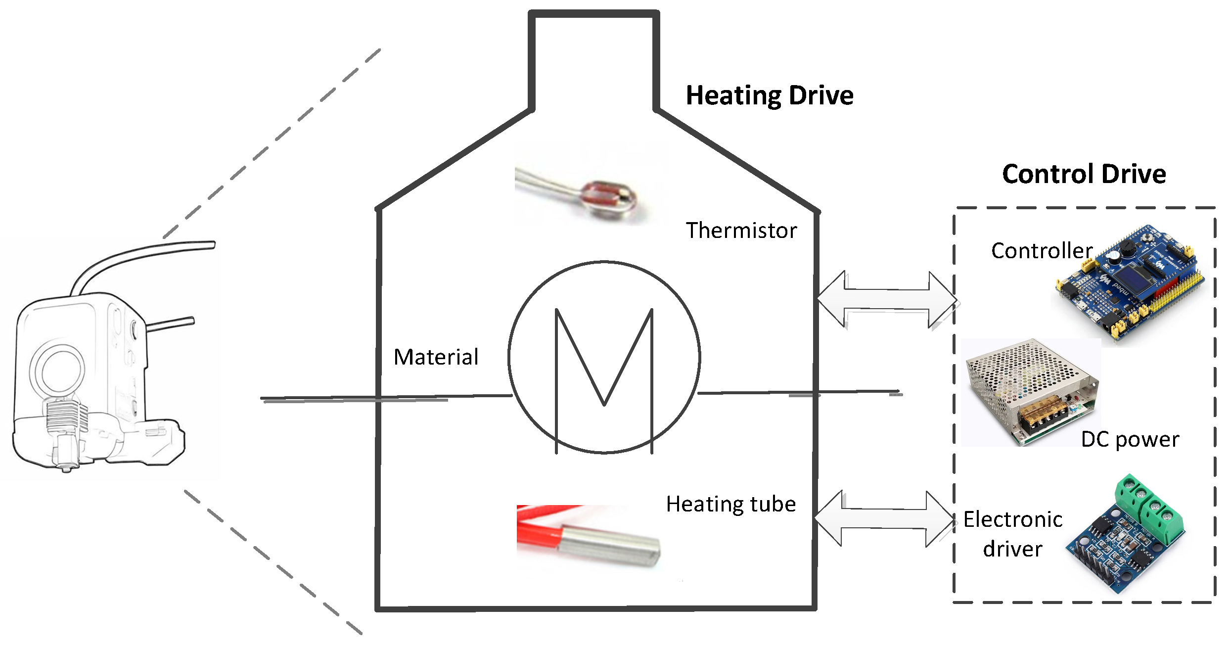
2.1. Uncooled Heating Processes

Considering a second-order heating device with significant inertia that lacks a cooling system, the situation can be described as follows:

$$\ddot{y}=a_1\dot{y}+a_{0}y+b(u+d)$$

(1)

where $u$ is the heating input, $y$ is the temperature measurement output, $d$ represents the unknown low-frequency disturbances, and $a_0>0,a_1>0,b>0$ denotes the unknown parameters of the heating device. Since the heating device lacks a cooling control mechanism, the control input is always in a non-negative state, $u\ge 0$; when $u=0$, the temperature process is in a natural cooling state.

Once the temperature reaches the set point, there theoretically exists a small control input $u^{*}$ that balances the heating and cooling processes. However, it is challenging for the actual heating process to quickly converge to the ideal control state, and this equilibrium state varies with changes in the ambient temperature. Therefore, preventing overshoot and oscillation in such uncooled heating devices has become a difficult issue to address.

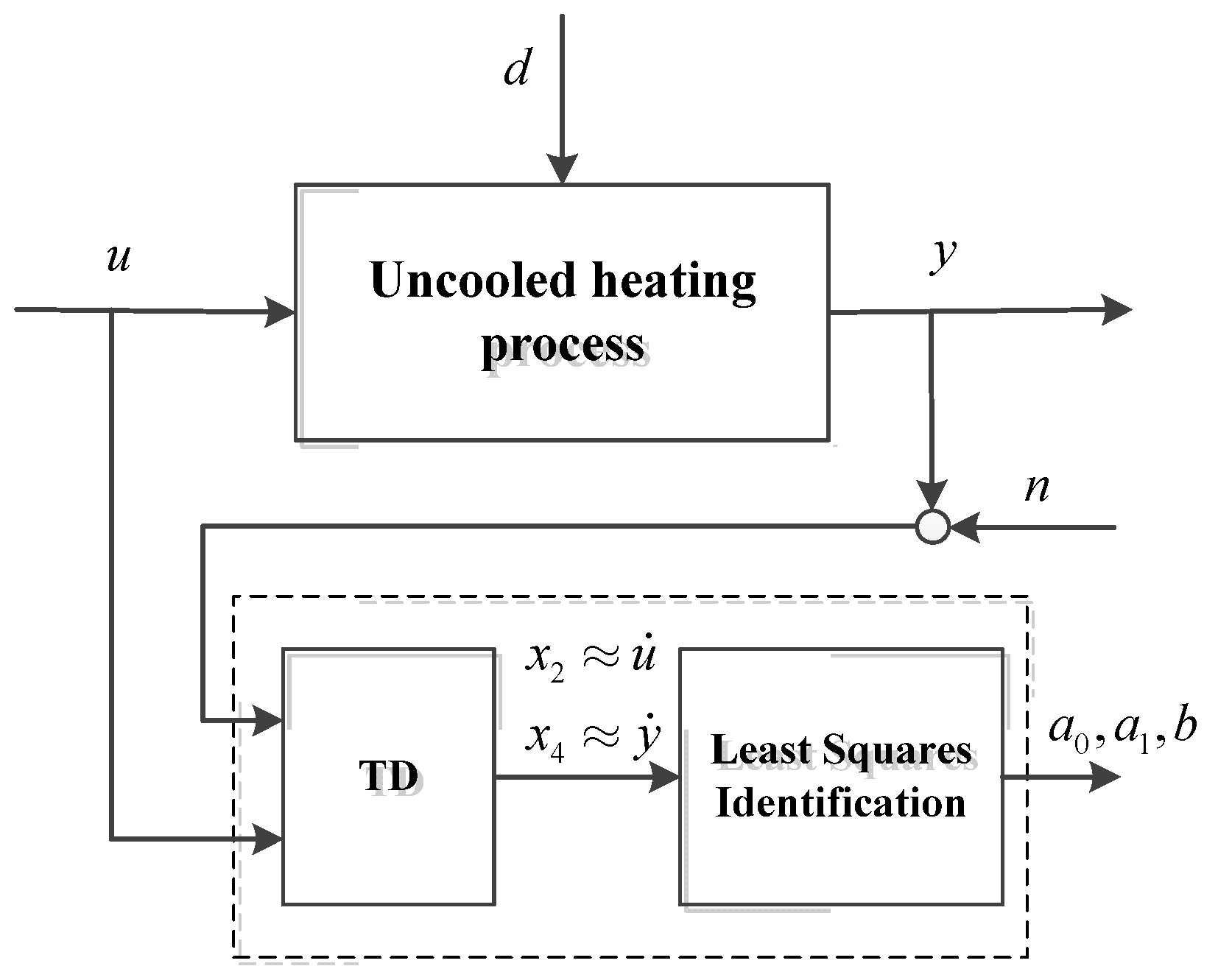
2.2. TD-Based Identification Method against Disturbance

When faced with unknown disturbances, the identification of heating equipment must be robust enough to yield accurate models that can withstand the effects of such perturbations. This process is essential for developing control strategies that can effectively counteract the disturbances and maintain the system’s stability and performance.

The presence of unknown disturbances introduces uncertainties into the model identification phase, which can significantly affect the accuracy of the model parameters. For system (1), if $d=0$ is known, the least squares method can be used for the unbiased identification of the unknown parameters $a_0,a_1,b$. However, when $d\ne 0$ is not known, external disturbances can bias the identification results, potentially making them entirely different from the original system characteristics. Therefore, this paper proposes to study an anti-disturbance identification method based on a tracking differentiator to overcome the impact of disturbances.

By expressing (1) as a transfer function model, we have,

$$G(s)={\displaystyle \frac{y(s)}{u(s)+d(s)}}={\displaystyle \frac{b}{s^2+a_{1}s+a_0}}$$

(2)

Since changes in the external environment are relatively slow, the equivalent disturbance $d$ has low-frequency characteristics, denoted as $\dot{d}\approx 0$. After differentiating the input and output signals, they can still represent the dynamic characteristics of the system, as shown in:

$${\displaystyle \frac{sy(s)}{su(s)+sd(s)}}\approx {\displaystyle \frac{sy(s)}{su(s)}}=G(s)$$

(3)

According to (3), if the derivative signal $\dot{u},\dot{y}$ can be obtained, the system model $G(s)$ can be identified. The anti-disturbance identification scheme proposed in this paper is illustrated in Figure 1.

Direct differentiation processing can amplify the noise present in the system; therefore, a tracking differentiator (TD) is employed to extract the derivative signal from the system. Given a sampling period $T$, a discrete two-input and two-output TD is constructed based on the principle of the tracking differentiator [13]:

$$TD:\{\begin{array}{l}\dot{x}(k)=(AT+I)x(k-1)+BT\zeta (k-1)\\ \dot{\zeta }(k)\approx Cx(k)\end{array}$$

(4)

where $x={\left[\begin{array}{cccc}{x}_1& x_2& x_3& x_4\end{array}\right]}^T$, $\zeta ={\left[\begin{array}{cc}u& y\end{array}\right]}^T$,

$$\begin{array}{l}\overline{A}=\left[\begin{array}{cccc}0& 1& 0& 0\\ -{\omega }_o^2& -2{\omega }_o& 0& 0\\ 0& 0& 0& 1\\ 0& 0& -{\omega }_o^2& -2{\omega }_o\end{array}\right],\\ \overline{B}=\left[\begin{array}{cc}0& 0\\ {\omega }_o^2& 0\\ 0& 0\\ 0& {\omega }_o^2\end{array}\right],\overline{C}={\left[\begin{array}{cc}0& 0\\ 1& 0\\ 0& 0\\ 0& 1\end{array}\right]}^T\end{array}$$

where ${\omega }_o$ is a bandwidth parameter of the TD and is a key factor. The larger the value of ${\omega }_o$, the faster the differentiation tracking speed, while also serving as a filter to eliminate the effects of noise. Therefore, it is necessary to properly choose the value of ${\omega }_o$ to balance the requirements for speed and filtering. Within the TD, the following relationship holds, $\dot{u}\approx x_2,\dot{y}\approx x_4$.

Incorporating the principle of derivative identification from Equation (3), and using $\dot{u}\approx x_2,\dot{y}\approx x_4$ as the input and output, system (1) is discretized to obtain:

$$\begin{array}{l}{x}_4(k)=\underset{{\theta }_1}{\underbrace{-(a_{1}T-2)}}{x}_4(k-1)\\ \underset{{\theta }_2}{\underbrace{-(1-a_{1}T+a_0{T}^2)}}{x}_4(k-2)+\underset{{\theta }_3}{\underbrace{b{T}^2}}{x}_2(k-2)\end{array}$$

Construct the data vector $\phi (k)$ and the parameter vector $\theta (k)$

$$\phi (k)=\left[\begin{array}{ccc}-x_4(k-1)& -x_4(k-2)& x_2(k-2)\end{array}\right]$$

$$\theta (k)=\left[\begin{array}{ccc}{\theta }_1& {\theta }_2& {\theta }_3\end{array}\right]$$

Construct the output matrix $\Pi$ and the regression matrix $\Phi$

$$\Pi =\left[\begin{array}{c}{x}_4(1)\\ x_4(2)\\ ⋮\\ x_4(L)\end{array}\right],\Phi =\left[\begin{array}{c}{\phi }^T(1)\\ {\phi }^T(2)\\ ⋮\\ {\phi }^T(k)\end{array}\right]$$

Using the least squares estimation (LSE), an estimate of the parameter vector $\theta$ can be obtained

$$\tilde{\theta }={\left({\Phi }^T\Phi \right)}^{-1}{\Phi }^T\Pi$$

Transforming $\tilde{\theta }$ into a parameterized form of the system, we have

$$\left[\begin{array}{ccc}{a}_1& a_0& b\end{array}\right]=\left[\begin{array}{ccc}{\displaystyle \frac{-{\tilde{\theta }}_1+2}{T}}& {\displaystyle \frac{-{\tilde{\theta }}_1-{\tilde{\theta }}_2+1}{T^2}}& {\displaystyle \frac{{\tilde{\theta }}_3}{T^2}}\end{array}\right]$$

(5)

The pseudocode of TD-based identification method is given as Algorithm 1.

Algorithm 1: Anti-disturbance Identification based on TD

Input: Input signal ($u$), Sampling period ($T$ s), Bandwidth parameter (${\omega }_o$). Output: Identified model parameters ( $[a_1 a_0 b]$). 1: Operate TD (4) with bandwidth ${\omega }_o$; 2: Collect the data $x_2(kT),x_4(kT), t=kT,k=0,1,\cdots ,N$; 3: Construct data matrix: $\phi (k),\Pi ,\Phi$; 4: Perform LSE with $\phi (k),\Pi ,\Phi$ to identify model parameters $\tilde{\theta }$; 5: Calculate $[a_1 a_0 b]$ by (5).

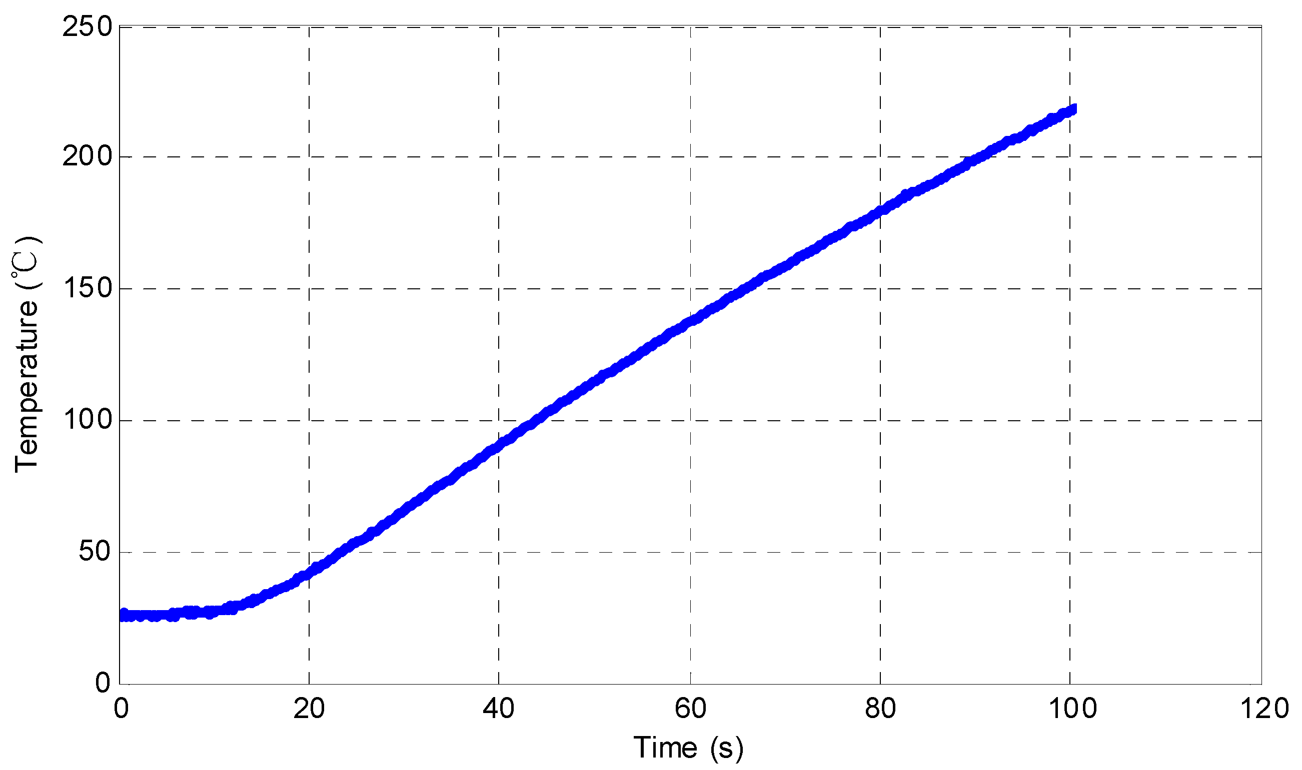
2.3. Identification Results

For a class of uncooled heating experimental subjects, an open-loop step test is conducted to obtain input and output data for system model identification. The routine operating temperature of the heating process is around $200$ °C; to fully activate the system characteristics, the heater input is set to $u=12$ V, and the measured temperature data is recorded as $y$. Due to the temperature protection limitations of the physical system, only temperature data within the range of $0-220$ °C can be collected, with a sampling time of $T=0.5$ s. The actual measured temperature curve of the system is shown in Figure 2.

Utilizing the proposed anti-disturbance identification algorithm and taking ${\omega }_o=50$, the TD is constructed to identify the system transfer function, resulting in

$$G(s)={\displaystyle \frac{59}{3835s^2+247.7s+1}}$$

(6)

Equation (6) describes the heating dynamics during $u>0$, where there is significant inertia from the change in the heater input to the temperature change. When $u=0$, although heating is no longer applied, the cooling process through air cooling with no active cooling measures is very slow. To achieve precise and rapid temperature adjustment, it is required that the control quantity $u$ can be reduced in advance. Therefore, it is necessary to combine the temperature dynamic model to study the temperature control strategy suitable for uncooled heating conditions.

By implementing the TD-based identification, the obtained model (6) serves as a foundation for designing control systems. This leads to improved control performance and ensures the system’s robustness in the face of real-world operational conditions.

3. Uncooled Control Constraints and Temperature Prediction Control

3.1. Uncooled Control Constraints

Firstly, to adapt to the operating conditions without cooling, it is necessary to impose restrictions on the control input of the heating device to prevent significant overshoot and temperature fluctuations. This paper considers two types of constraints for the heating device. One, is the constraint on the control input $u$, i.e., hardware amplitude limitations; for example, the maximum voltage of the heater here is 12 V. The other is the constraint on the changes in the control input $\Delta u$, which requires that the adjustments to the heater should not be too large to ensure smooth temperature changes.

To this end, consider the unilateral constraint on the control input,

$$0\le u(k)=u(k-1)+\Delta u(k)\le u^{\max }$$

where $u(k)=0$ corresponds to the air-cooling process, and $u(k)>0$ corresponds to the heating process. Write the constraint conditions within the control range $N_c$ in vector form, we have

$$M_1\Delta U\le N_1$$

where $M_1$ and $N_1$ are the constraint matrices, and $\Delta U$ is the vector within $N_c$ of $\Delta u$.

Consider the constraint on the changes in the control input $\Delta u$:

$$\left|\Delta u(k)\right|\le \Delta u^{\max }$$

Writing the constraint conditions within the control range $N_c$ in vector form, we have:

$$M_2\Delta U\le N_2$$

where $M_2$, $N_2$ are the constraint matrix. Let $M={[M_1,M_2]}^T$ and $N={[N_1,N_2]}^T$, we have

$$M\Delta U\le N$$

(7)

Constraint condition (7) can overcome the overshoot caused by rapid adjustment but still cannot produce advanced control actions. With the known control input $u$, the system model (6) can predict the temperature change, which also provides a basis for the advanced action of the control input, which is the essence of predictive control thinking.

3.2. Input-Constrained Temperature Prediction Control (ICTPC)

To generate the effect of anticipatory control adjustments, the system model (6) is utilized to predict temperature changes [20,21,22,23]. It is assumed that the discrete state-space model $\left(A_m, B_m, C_m\right)$ is given, with the state represented as $x_m(k)$. To introduce integration that eliminates steady-state errors, the state-space model is rewritten as a difference model, forming new state variables $x(k)$ and the system matrix $\left(A, B, C\right)$

$$\{\begin{array}{c}\stackrel{x(k+1)}{\overbrace{\left[\begin{array}{c}\Delta x_m(k+1)\\ y(k+1)\end{array}\right]}}=\stackrel{A}{\overbrace{[\begin{array}{c}{A}_m\\ C_m{A}_m\end{array}\begin{array}{l}{o}_m^T\\ 1\end{array}]}}\stackrel{x(k)}{\overbrace{\left[\begin{array}{c}\Delta x_m(k)\\ y(k)\end{array}\right]}}+\stackrel{B}{\overbrace{\left[\begin{array}{c}{B}_m\\ C_m{B}_m\end{array}\right]}}\Delta u(k)\\ y(k)=\stackrel{C}{\overbrace{[o_{m}1]}}\left[\begin{array}{c}\Delta x_m(k)\\ y(k)\end{array}\right]\end{array}$$

where $o_m$ is a zero matrix of the appropriate size. The system sampling period is 0.5 s, and the resulting system matrix is

$$A=\left[\begin{array}{ccc}0.9796& 0& 0\\ 0.4949& 1& 0\\ 0.0055& 0.0111& 1\end{array}\right], B=\left[\begin{array}{c}0.4949\\ 0.1241\\ 0.0014\end{array}\right], C={\left[\begin{array}{c}0\\ 0\\ 1\end{array}\right]}^T$$

The current moment is $k$, with a given control horizon of $N_c$ (computing the next $N_c$ steps $\Delta u$), and the prediction horizon $N_p$ (predicting the next $N_p$ state quantities from the current state variables $x(k)$), and generally $N_c<N_p$. Assuming that the control input changes to zero outside the control horizon, we have:

$$\Delta u(k+i)=0,i=N_c,N_c+1,\cdots ,N_p-1,$$

Then the approximate result of the state variables is as follows:

$$\begin{array}{l}x(k+N_p)=A^{N_p}x(k)+A^{N_p-1}B\Delta u(k)\\ +A^{N_p-2}B\Delta u(k+1)+\cdot \cdot \cdot \cdot \cdot \cdot +A^{N_p-N_c}B\Delta u(k+N_c-1)\end{array}$$

To further obtain the predicted output, the output can be written in matrix form:

$$\{\begin{array}{l}y(k+1)=CAx(k)+CB\Delta u(k)\\ y(k+2)=C{A}^{2}x(k)+CAB\Delta u(k)+CB\Delta u(k+1)\\ \cdot \cdot \cdot \cdot \cdot \cdot \\ y(k+N_p)=C{A}^{N_p}x(k)+C{A}^{N_p-1}B\Delta u(k)+C{A}^{N_p-2}B\Delta u(k+1)\\ +\cdot \cdot \cdot \cdot \cdot \cdot +C{A}^{N_p-N_c}B\Delta u(k+N_c-1)\end{array}$$

The output is formulated in matrix form

$$Y=Fx(k)+\varphi \Delta U$$

(8)

$$Y={\left[y(k+1),y(k+2),\cdot \cdot \cdot y(k+N_p)\right]}^T,$$

$$\Delta U={\left[\Delta u(k),\Delta u(k+1),\cdot \cdot \cdot \Delta u(k+N_c-1)\right]}^T,$$

$$F=\left[\begin{array}{c}CA\\ C{A}^2\\ C{A}^2\\ \cdot \cdot \cdot \\ C{A}^{N_p}\end{array}\right];\varphi =\left[\begin{array}{ccccc}CB& 0& 0& \dots & 0\\ CAB& CB& 0& \dots & 0\\ C{A}^{2}B& CAB& CB& \dots & 0\\ \dots & & & & \\ C{A}^{N_p-1}B& C{A}^{N_p-2}B& C{A}^{N_p-3}B& \dots & C{A}^{N_p-N_c}B\end{array}\right]$$

Given an initial system temperature $y_0$ and a desired temperature of $y^{*}$, a reference trajectory can be generated using $y_s(t)=y_0+(y^{*}-y_0)(1-e^{-\tau t})$, where $\tau$ represents the transition time, and the resulting sequence is denoted as $Y_s^T$. Incorporating the constraint conditions, the sequence $\Delta U$ can be determined by solving the following optimization problem:

$$\begin{array}{l}\min J={(Y_s-Y)}^T(Y_s-Y)+\Delta U^T\overline{R}\Delta U\\ s.t.M\Delta U\le N\end{array}$$

(9)

In Equation (9), the first term represents the error between the input and output; the second term is to prevent excessive action of the control signal, which is a constraint on the control signal, where $\overline{R}$ is the weighting matrix. For the quadratic programming problem in (9), methods such as the Lagrange multiplier method and the interior point method can be used to solve it.

According to the principle of predictive control, the first element of $\Delta U$ is used to update the current control quantity, $\Delta u(k)=\left[\begin{array}{cccc}1& 0& \cdots & 0\end{array}\right]\Delta U$. Following the aforementioned method, the control quantity is optimized in a rolling manner for each moment.

4. Temperature Control and Experimental Results

4.1. Experiment Conditions

Industrial devices, such as resistive heaters and ceramic heaters, are a typical class of uncooled heating equipment, specifically designed for heating various production materials (such as metals, ores, chemicals, etc.). Their working mechanism is entirely based on the heating process and does not involve any cooling mechanism.

The experimental prototype device utilized in our study is the heating extrusion head of a 3D printer, which serves as a practical example of uncooled heating equipment. We constructed the experimental device by meticulously selecting and integrating the appropriate components, closely following the design of this prototype system to ensure accurate replication and functionality. The experimental system is constructed as shown in Figure 3.

In our experimental setup, we utilized the STC12C5A60S2 microcontroller, known for its high processing speed and robustness in handling analog and digital signals. This microcontroller was selected for its ability to accurately control the heating process and to process temperature data in real-time. A detailed wiring diagram is provided in Figure 3, which illustrates the connections between the microcontroller, the NTC thermistor, the L298N driver chip, and the 12 V, 40 W single-headed electric heating tube. Each component’s role and specifications are described in detail in the following section, ensuring that the setup can be replicated for further studies.

The heater in the experimental system is a single-headed electric heating tube (12 V, 40 W), and the temperature sensing device is a thermistor (NTC R25). The cooling method in the heating device is air cooling with no active cooling measures. Equation (6) provides the identification model of the heating device.

The control system has a sampling period of 0.5 s, and the control input is constrained by $0\le u<12$ V. To prevent excessive heating actions when the temperature is close to the set value, constraints are imposed on the changes in the control input. In the experiment, $\Delta u^{\max }$ is given to verify the control performance under different values.

4.2. Weight Design in Controller

Due to the long response time of the system, a long prediction period is selected. To reduce computational effort, the prediction horizon $N_p=100$ and the control horizon $N_c=2$ are selected with $\overline{R}=r_w{I}_{Nc\times Nc},r_w>0$. $\Delta u^{\max }=2$ is chosen to limit the changes in the control input.

Selecting the weight parameter $r_w$ is crucial for our control algorithm’s performance, as it balances response speed with stability. We fine-tune this parameter through a systematic experimental process, beginning with lower values that offer quick responses but can cause overshoot and oscillations. By gradually increasing the weight and evaluating the system’s behavior at each step, we find the optimal value that meets our criteria for minimizing overshoot and oscillations while maintaining a swift response to set point changes. Figure 4 shows the control curves under three different values, $r_w=0$, $r_w=10$ and $r_w=20$. It can be seen from Figure 4 that after the introduction of weighting, the overshoot and oscillation of the temperature control curve are significantly reduced. The larger the $r_w$, the more cautious the change in control quantity each time, i.e., $\Delta u$ will be smaller, making the steady state of the temperature process more stable. On the other hand, a larger $r_w$ will also slow down the temperature response speed during the heating process, mainly reflected in the dynamic process of temperature change. It can be seen that increasing the weight of the control quantity constraint is a control method that overcomes the system’s overshoot and oscillation at the expense of the system’s response speed. For air-cooled heating devices working in a steady state, this method is very practical. Therefore, this paper selects $r_w=20$ as the controller parameter.

In the experiment, $\Delta u^{\max }$ is taken as 0.5, 1, and 1.5 to verify the impact of different upper limits of control quantity constraints on control performance. The experimental results are shown in Figure 5. $\Delta u^{\max }$ that is too small results in significant steady-state errors, while a $\Delta u^{\max }$ that is too large causes system overshoot. Therefore, based on the experimental results, a $\Delta u^{\max }=1$ selected that reduces steady-state errors while suppressing steady-state oscillations.

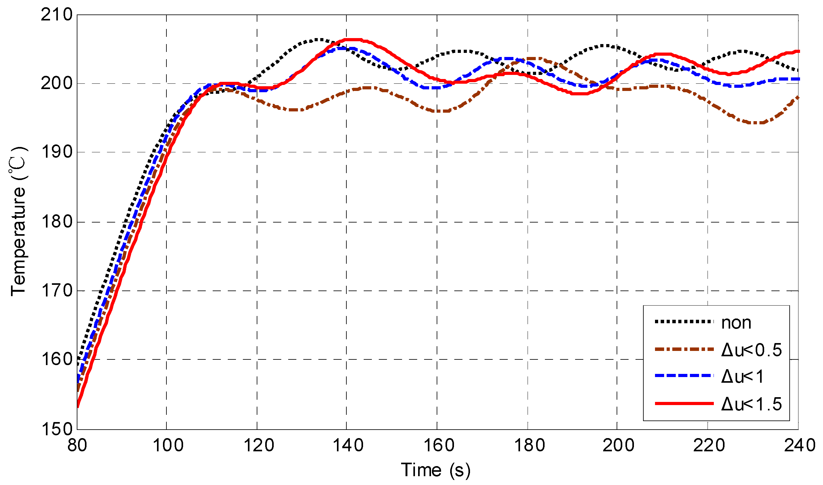
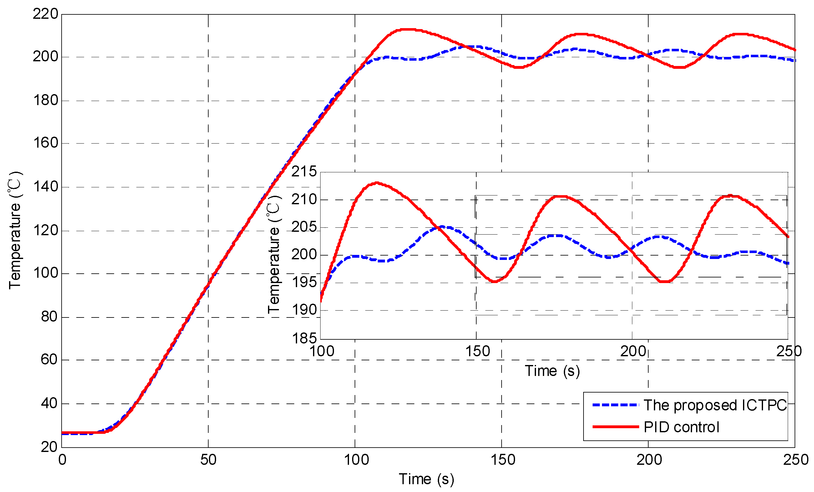
4.3. Experimental Results and Comparisons

To validate the effectiveness of the method presented in this paper, a temperature regulation experiment was conducted using the designed constrained temperature prediction controller, with $r_w=20$ and $\Delta u^{\max }=1$, the target temperature was set to 200 °C. Concurrently, a classical PID controller was designed

$$C(s)=K_p+{\displaystyle \frac{K_i}{s}}+K_{d}s$$

serving as a benchmark for evaluating the performance of our proposed method. The PID controller was implemented by tuning the controller gains to achieve a balance between response speed and stability. With carefully tuned, $K_p=0.42,K_i=0.001,K_d=6.5$ are used in the experiment to manage the heating processes effectively. The experimental results of the two types of controllers are shown in Figure 6.

From Figure 6, it can be seen that even though the response speeds of the two controllers are consistent, the overshoot of the PID control is significantly greater than that of the method in this paper. The reason is that the PID control can only react after the deviation occurs. When the temperature approaches the target value, although the derivative action can produce a certain deceleration effect, due to the lack of a cooling process, the PID cannot produce an accurate reverse regulation effect, causing the temperature to continue to increase. In addition, the conventional PID controller does not integrate the system’s dynamic characteristics and lacks a control constraint mechanism, thus it cannot better overcome the overshoot and oscillation of the highly inertial system. However, the design method proposed in this paper fully considers the heating characteristics under the condition of no cooling, introduces control constraints in a targeted manner, and makes the temperature enter the steady state as smoothly as possible. The comparative performance of the two control methods is presented in

Table 1. Control performance comparisons of two controllers in the experiments.

Control Strategy	Overshoot	Peak Time	Steady-State Error
PID control	7.1%	118 s	11 °C
The proposed ICTPC	3.0%	110 s	4 °C

.

5. Conclusions

In this work, we have studied the complex issue of temperature regulation in uncooled heating systems, which are typically characterized by the absence of active cooling mechanisms and are prone to temperature oscillations. Our research has led to the development of an anti-disturbance identification method by using tracking differentiator (TD), complemented by a predictive control framework that incorporates control input constraints. This integrated approach has been instrumental in achieving high performance-control in the absence of active cooling.

The proposed approach not only enhances the robustness of the system against disturbances but also provides a practical solution for temperature control in systems without cooling capabilities. Future work will focus on extending this approach to a broader class of industrial heating processes and exploring its integration with advanced sensor networks and machine learning algorithms for enhanced predictive capabilities.

References

1. Seborg, D.E.; Edgar, T.F.; Mellichamp, D.A.; Doyle, F.J., III. Process Dynamics and Control; John Wiley & Sons: Hoboken, NJ, USA, 2016. [Google Scholar]
2. Pastukhov, V.G.; Maydanik, Y.F. Temperature control of a heat source using a loop heat pipe integrated with a thermoelectric converter. Int. J. Therm. Sci. 2023, 184, 108012. [Google Scholar] [CrossRef]
3. Grassi, E.; Tsakalis, K. PID controller tuning by frequency loop-shaping: Application to diffusion furnace temperature control. IEEE Trans. Control. Syst. Technol. 2000, 8, 842–847. [Google Scholar] [CrossRef]
4. Kumavat, M.; Thale, S. Analysis of CSTR Temperature Control with PID, MPC & Hybrid MPC-PID Controller. In Proceedings of the International Conference on Automation, Computing and Communication 2022 (ICACC-2022), Nerul, India, 7–8 April 2022; p. 01001. [Google Scholar]
5. Taler, D.; Sobota, T.; Jaremkiewicz, M.; Taler, J. Control of the temperature in the hot liquid tank by using a digital PID controller considering the random errors of the thermometer indications. Energy 2022, 239, 122771. [Google Scholar] [CrossRef]
6. Panda, R.C.; Yu, C.C.; Huang, H.P. PID tuning rules for SOPDT systems: Review and some new results. ISA Trans. 2004, 43, 283–295. [Google Scholar] [CrossRef] [PubMed]
7. Nie, Z.Y.; Li, Z.; Wang, Q.G.; Gao, Z.; Luo, J. A unifying Ziegler–Nichols tuning method based on active disturbance rejection. Int. J. Robust Nonlinear Control. 2022, 32, 9525–9541. [Google Scholar] [CrossRef]
8. Vanavil, B.; Chaitanya, K.K.; Rao, A.S. Improved PID controller design for unstable time delay processes based on direct synthesis method and maximum sensitivity. Int. J. Syst. Sci. 2015, 46, 1349–1366. [Google Scholar] [CrossRef]
9. Shamsuzzoha, M.; Lee, M. IMC−PID controller design for improved disturbance rejection of time-delayed processes. Ind. Eng. Chem. Res. 2007, 46, 2077–2091. [Google Scholar] [CrossRef]
10. Huang, H.; Zhang, S.; Yang, Z.; Tian, Y.; Zhao, X.; Yuan, Z.; Hao, S.; Leng, J.; Wei, Y. Modified smith fuzzy pid temperature control in an oil-replenishing device for deep-sea hydraulic system. Ocean. Eng. 2018, 149, 14–22. [Google Scholar] [CrossRef]
11. Duan, X.G.; Deng, H.; Li, H.X. A Saturation-Based Tuning Method for Fuzzy PID Controller. IEEE Trans Ind. Electron. 2013, 60, 5177–5185. [Google Scholar] [CrossRef]
12. Liu, R.; Nie, Z.Y.; Shao, H.; Fang, H.; Luo, J.L. Active disturbance rejection control for non-minimum phase systems under plant reconstruction. ISA Trans. 2023, 134, 497–510. [Google Scholar] [CrossRef] [PubMed]
13. Huang, C.E.; Li, D.; Xue, Y. Active disturbance rejection control for the ALSTOM gasifier benchmark problem. Control. Eng. Pract. 2013, 21, 556–564. [Google Scholar] [CrossRef]
14. Zhang, R.; Zou, Q.; Cao, Z.; Gao, F. Design of fractional order modeling based extended non-minimal state space MPC for temperature in an industrial electric heating furnace. J. Process Control 2017, 56, 13–22. [Google Scholar] [CrossRef]
15. Ramasamy, V.; Kannan, R.; Muralidharan, G.; Sidharthan, R.K.; Veerasamy, G.; Venkatesh, S.; Amirtharajan, R. A comprehensive review on Advanced Process Control of cement kiln process with the focus on MPC tuning strategies. J. Process Control 2023, 121, 85–102. [Google Scholar] [CrossRef]
16. Li, J.; Yang, S.; Yu, T.; Zhang, X. Data-driven optimal PEMFC temperature control via curriculum guidance strategy-based large-scale deep reinforcement learning. IET Renew. Power Gener. 2022, 16, 1283–1298. [Google Scholar] [CrossRef]
17. Nie, Z.Y.; Li, G.M.; Yan, L.C.; Wang, Q.G.; Luo, J.L. On disturbance rejection proportional–integral–differential control with model-free adaptation. Control. Theory Technol. 2023, 21, 34–45. [Google Scholar] [CrossRef]
18. Aslam, S.; Hannan, S.; Zafar, W.; Sajjad, M.U. Temperature control of water-bath system in presence of constraints by using MPC. Int. J. Adv. Appl. Sci. 2016, 3, 62–68. [Google Scholar] [CrossRef]
19. Han, J. From PID to Active Disturbance Rejection Control. IEEE Trans. Ind. Electron. 2009, 56, 900–906. [Google Scholar] [CrossRef]
20. Rawlings, J.B.; Mayne, D.Q. Model Predictive Control: Theory and Design; Nob Hill Pub., LLC: Madison, WI, USA, 2009. [Google Scholar]
21. Rawlings, J.B. Tutorial overview of model predictive control. IEEE Control. Syst. Mag. 2002, 20, 38–52. [Google Scholar]
22. Bhavsar, S.; Kant, K.; Pitchumani, R. Robust model-predictive thermal control of lithium-ion batteries under drive cycle uncertainty. J. Power Sources 2023, 557, 232496. [Google Scholar] [CrossRef]
23. Li, Z.; Wang, X.; Du, W.; Yang, M.; Li, Z.; Liao, P. Data-driven adaptive predictive control of hydrocracking process using a covariance matrix adaption evolution strategy. Control. Eng. Pract. 2022, 125, 105222. [Google Scholar] [CrossRef]
Figure 1. TD-based identification against disturbance.
Processes 12 02137 g001
Figure 2. Heating Device Test.
Processes 12 02137 g002
Figure 3. Heating system for experiments.
Processes 12 02137 g003
Figure 4. Experimental results under different weights.
Processes 12 02137 g004
Figure 5. Experimental results with different constraints.
Processes 12 02137 g005
Figure 6. Experimental results and comparison.
Processes 12 02137 g006