Abstract
In hard disk drive (HDD) manufacturing, a reflow soldering process (RSP) employs heat generated at the welding tip (WT) to bond tiny electrical components for assembling an HDD. Generally, the heat was generated by an electric current applied to the WT. This article reports a feasibility study of using hot air based on computational fluid dynamics (CFD), a choice to assist heat generation. First, the WT and hot air tube (HAT) prototypes were designed and created. The HAT is a device that helps to supply hot air directly to generate heat at the WT. Then, the experiment was established to measure the temperature (T) supplied by the hot air. The measure results were employed to validate the CFD results. Next, the prototype HAT was used to investigate the T generated at the WT by CFD. The comparison revealed that the T measured by the experiment was in the 106.2 °C–133.5 °C range and that the CFD was in the 107.3 °C–136.6 °C range. The maximum error of the CFD results is 2.3% compared to the experimental results, confirming the credibility of the CFD results and methodology. The CFD results revealed that the operating conditions, such as WT, HAT designs, hot air inlet velocity, and inlet temperature, influence the T. Last, examples of suitable operating conditions for using hot air were presented, which confirmed that hot air is a proper choice for a low-temperature RPS.
1. Introduction
In 2017–2021, Thailand was ranked as the second largest hard disk drive (HDD) exporter globally, with an average value of USD 6,384 million per year, about 223,440 million baht per year [1,2] (1 USD for 35 THB). It was around 1.39% of Thailand’s export value; therefore, Thailand is a major HDD manufacturer base, with leading manufacturing technology that is developed domestically [3]. One of the technologies is a reflow soldering process (RSP) technology.
Conventionally, the RSP in HDD manufacturing uses heat generated at the welding tip (WT) by applying an electric current to the WT to melt solder balls for joining a flexible printed circuit (FPC) with a printed circuit cable (PCC) to assemble a head stack assembly (HSA) [4,5,6]. Based on Joule’s heating principle with suitable operating conditions, the applied current generates a high temperature of about 300 °C–500 °C at the WT, sufficient for an HSA assembly. Figure 1 shows the RSP: (a) a location in the HSA and (b) an enlarged picture focusing on the FPC and PCC. The significant advantage of the RSP using the applied current is that it can generate a high temperature quickly; for example, from 30 °C to 500 °C within 0.7 s, as reported in [4,5,6]. In contrast, the disadvantages are that it requires complex and expensive equipment, is unsuitable for melting at a low temperature, and has product defects due to uneven temperatures at the welding points [5]. Figure 2 shows a sample of the WT for the RSP: (a) an actual model and (b) a CAD model with mocking temperature. The small picture in (b) presents an overview model, while the large one focusing on the welding points presents the mocking temperature due to the RSP. It was found from the actual RSP using an applied current led to uneven temperature at the welding points, as depicted in Figure 2b. The center had a higher temperature than the border; solder balls were melted only in the middle and not melted at the border, causing defects in some products. The size of the solder is about 0.1–0.2 mm2, depending on the product welding points.
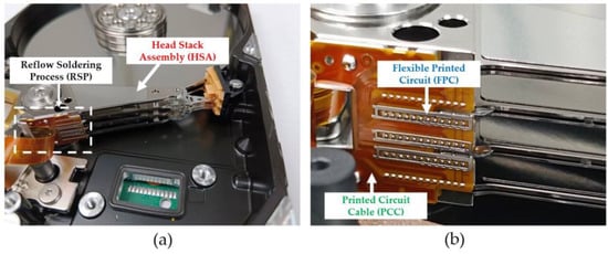
Figure 1.
The RSP: (a) a location in the HSA and (b) an enlarged picture focusing on the FPC and PCC.
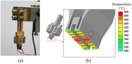
Figure 2.
A sample of the WT for the RSP: (a) an actual model and (b) a CAD model with a mocking temperature for joining the FPC and PCC.
To avoid product defects, the temperature at the WT should be uniform. According to a literature review on the RSP [7,8,9,10,11,12,13,14], hot air is an interesting way to help distribute a uniform temperature at the welding points. Based on a forced convection heat transfer principle, when driving hot air/gas to a solid surface, heat is transferred between a solid surface and a fluid (air or gas) in motion, helping the temperature in a target surface distribute widely and evenly [7,8]. The hot-air RSP assists with greater bonding strength than the vacuum RSP in SAC305, lead-free solder alloy [9]. In addition, hot air is trendy in a hot-air solder leveling process. For example, in this process, high-pressure hot air is blown over the surface of a printed circuit board (PCB), removing excessive solder from its surface [10,11,12]. Another use for hot air is in a system in package (SiP) process. Forced convection due to hot gas/air was used in the SiP process for assembling two or more ICs inside a single package [13,14].
To achieve high efficacy in the hot-air RSP, computational fluid dynamics (CFD) has been employed to investigate the complex flow pattern in a reflow oven and heat transfer mechanism in the SiP assembly [13], to investigate the cooling stage of the RSP [15,16], and to predict the shape of the ball grid array due to the hot-air RSP [17]. The vital conclusions from the research in [13,14,15,16,17] revealed the key factors influencing the forced convection heat transfer due to hot air; for example, hot air velocity, hot air properties, devices releasing hot air, operating conditions, etc., which must be investigated for a high efficacy RSP on a case-by-case basis.
This article reports on the feasibility of using hot air in RSP instead of applied current, which has limitations in usage for HDD manufacturing based on CFD. Applied current provided an uneven temperature at the WT; hot air is a possible solution for this by generating an even temperature at the WT under suitable operating conditions. This article is a brief report from a project in which the authors collaborate with the HDD factory owning the problem. First, WT and hot air tube (HAT) prototypes were designed and created. Then, the measurement was established to measure the temperature at the WT due to the HAT. Next, CFD was employed to investigate the temperature and airflow in both prototypes. After that, the measurements and CFD results were compared to validate the CFD results and methodology credibility. Last, all results were analyzed to study the feasibility of using hot air in HDD manufacturing and determine suitable designs for HATs and the operating conditions.
The novel aspects of this research are the proper designs of the WT and HAT, with operating conditions that were developed and initially presented in this article, including recommendations for using hot air effectively. Since the CFD used the actual operating conditions from HDD manufacturing, these findings could be applied as essential information to develop a high-efficacy RSP in a collaborative factory.
2. Forced Convection Heat Transfer
This process may be called forced convection soldering [18] and involves the movement of fluid (liquid or gas) across a surface using external means, such as fans, pumps, or blowers, to enhance the heat transfer process. In brief, the governing equation of forced convection heat transfer is based on Newton’s law of cooling, expressed by [18]
where q is the heat transfer rate or heating power (W), A is the surface area (m2), TF is the undisturbed fluid temperature far from the surface (°C), TS is the surface temperature (°C), and h is the convection heat transfer coefficient (W/m2 K).
In fluid dynamics and heat transfer, the Nusselt number (Nu) is a dimensionless number representing the ratio of convective to conductive heat transfer across the boundary, such as the surface of a pipe, plate, or other object submerged in a fluid. The Nu is given by
where L is the characteristic length (m) and k is the fluid thermal conductivity (W/m °C).
The Nu is generally a function of the Reynold number (Re) and the Prandtl number (Pr) for the forced convection heat transfer. They are written by [19]
where ρ is the fluid density (kg/m3), µ is the dynamic viscosity (Pa s), cp is the specific heat (J/kg °C), and v is the fluid velocity.
Using Equations (1)–(5), it can be proved that
Equation (6) has no exact expression since all the parameters are related and depend on the operating conditions. To link with the RSP, Equation (6) implies that the q in the RSP depends on hot air velocity, the device shape through which hot air flows, and the hot air temperature. The higher the q, the better the forced convection heat transfer capability. This equation was used to validate the CFD results that are discussed in Section 4.
3. Methodology
The research methodology flowchart is presented in Figure 3, which includes prototypes of the WT and HAT, measurements, and the CFD process. The yellow boxes are the CFD process.
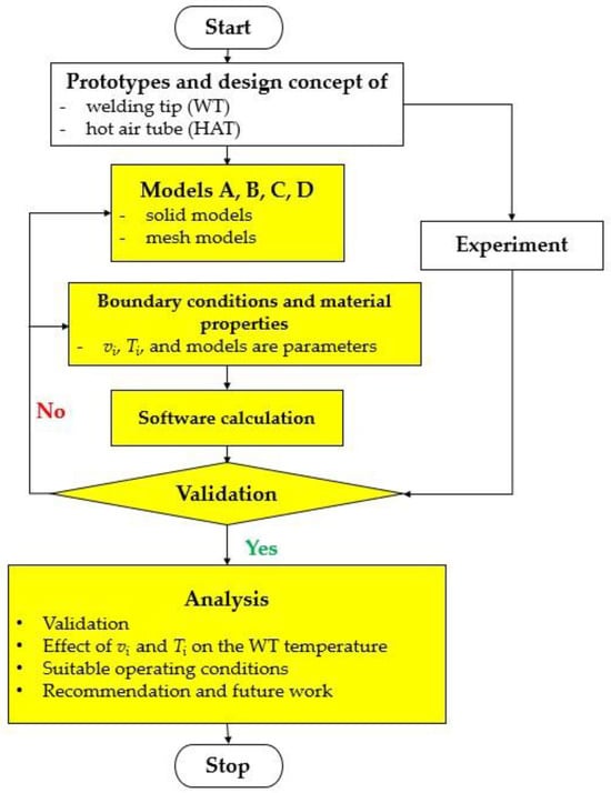
Figure 3.
The research methodology flowchart.
3.1. Prototype and Device Design Concepts
Since forced convection affects heat transfer in the WT, as explained in Equation (6), and nonuniform temperature causes product defects. A solution to avoid product defects is to design new devices with proper operating conditions to help distribute uniform temperature more evenly in the WT. Previously, hot air was not implemented in the actual HDD manufacturing in this factory; hence, the device prototypes used in this feasibility study of using hot air were newly designed and invented, as depicted in Figure 4, which includes a hot air tube (HAT) made of aluminum and a welding tip (WT) made of Haynes 230. The HAT functions to release hot air to generate the WT temperature and distribute it evenly, while the high temperature at welding points works to melt solder balls for bonding the FPC and PCC, as mentioned in Figure 1 and Figure 2. Both devices, the WT and HAT, work together under the operating conditions. The design concept of the HAT is to separate the hot air supplied by a hot air generator into two directions and let the hot air from both directions collide with the WT in the appropriate direction so that a high temperature is generated and evenly distributed. The red arrows in Figure 4 are the hot air directions obeying the mentioned design concept. The top hole is to supply hot air inside. As seen in Figure 2, the WT temperature is powered by the applied current, while in Figure 4, it is powered by the hot air. Figure 5 shows solid models with the rough dimensions of (a) the WT and (b) HAT prototypes.
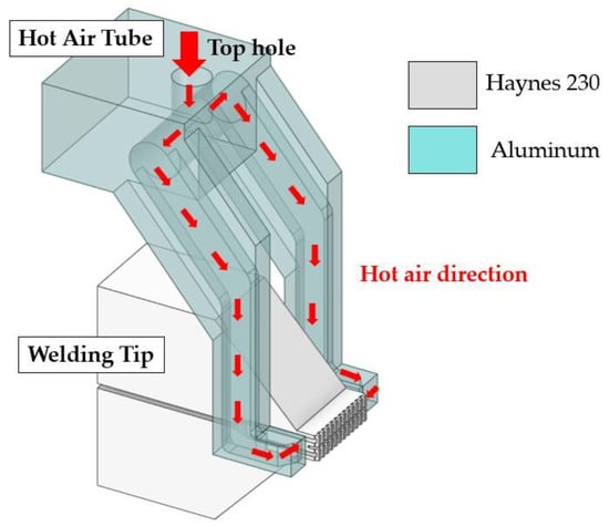
Figure 4.
The WT and HAT prototypes, including the hot air direction.
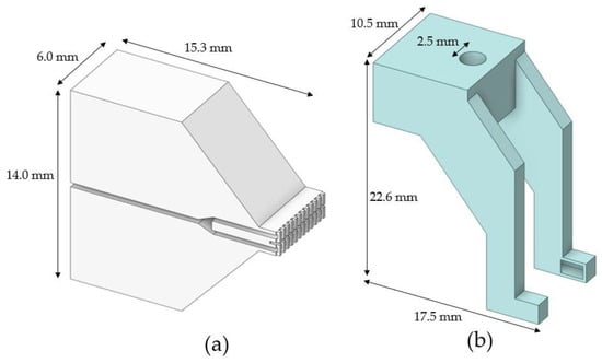
Figure 5.
The solid models with rough dimensions of (a) the WT and (b) HAT prototypes.
3.2. Experiment with Factory Operating Condition
An experiment was established to measure the WT temperature (T) heated by hot air, as shown in Figure 6. It includes an Optris PI-350 thermal imaging camera (Optris, Berlin, Germany), a computer with analysis software, a Hakko FM-206 hot air generator (Hakko, Osaka, Japan), an E-type thermocouple, and prototypes of the WT and HAT. The Optris PI-350 is a compact thermographic camera with an optical resolution of 282 × 288 pixels, can measure −20 °C–900 °C with an accuracy of ±2%, and works with analysis software. The Hakko FM-206 works as a hot-air generator that can release hot air with a maximum temperature of 550 °C and a maximum flow rate of 6 L/min. The thermocouple is a type E that can measure the temperature in the −270 °C to 870 °C range with an accuracy of ±0.5%. A computer with analysis software analyzes the data and records pictures sent from the Optris PI-350.
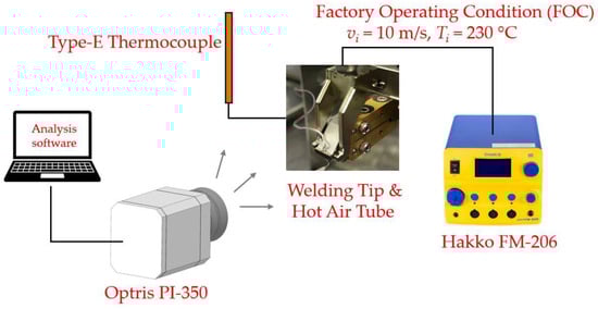
Figure 6.
The experiment.
The factory operating condition (FOC) for hot air supplied by the Hakko FM-206 is a velocity (vi) of 10 m/s and temperature (Ti) of 230 °C at the inlet. First, Hakko FM-206’s flow level was adjusted to release the hot air to the top hole of the HAT, as shown in Figure 4. The type-E thermocouple and the flow rate equation Q = viA, where Q is the flow rate (m3/s), vi is hot air velocity at the inlet, and A is the inlet cross section, were used to adjust the hot air properties vi and Ti to reach the FOC. At the FOC, the WT was heated by hot air, then the T was captured by the Optris PI-350. Last, the thermal data of T from the Optris PI-350 was sent to the computer to record the temperature and form the thermal picture using the analysis software. The experiment was performed at the FOC in only one case. The experimental results at the FOC are sufficient to validate the CFD results and research methodology, as later discussed in Section 4.1 of the validation.
3.3. Computational Fluid Dynamics (CFD)
3.3.1. Models
Four solid models, A–D, shown as transparent models in Figure 7, were created to determine the proper design of the HAT and the operating conditions for the RSP based on CFD. Importantly, all the models had nearly the same dimensions but differed in a few designs (presented as dark colors). The small pictures on the right reveal the different outlet shapes for releasing the hot air. In (a), model A has an identical shape and dimension to the prototype shown in Figure 4, Figure 5 and Figure 6. The outlet of model A in (a) is rectangular, while the outlet of model B in (b) is also rectangular but has thin top and bottom bars to force hot air to impact the WT directly (highlighted in orange). Models A and B have inner hollow tubes with rectangle cross sections for transporting hot air from the Hakko FM-206 to the WT. Models C and D have inner hollow tubes with circular cross sections. In addition, model D has the same outlet shape as model B.
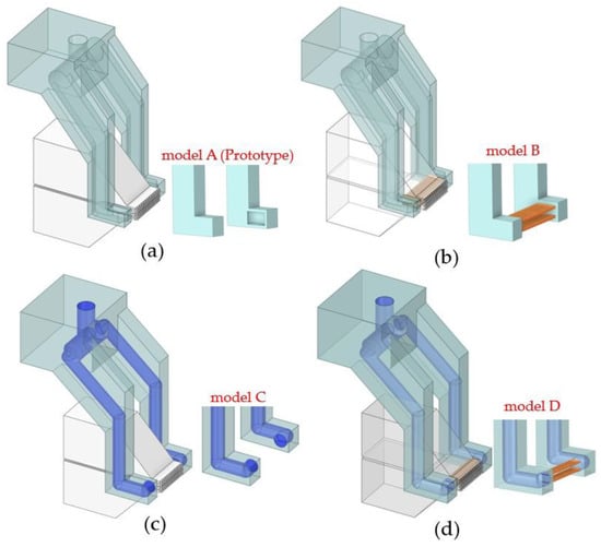
Figure 7.
The HAT designs of models A to D presented in (a–d), respectively.
Significantly, the CFD results using model A were later employed for comparison with the experimental results reported in Section 4.1 of the validation, and additional results using other models were used to determine the suitable model with operating conditions for a high-efficiency RSP in Section 4.3.
ANSYS Fluent meshing created mesh models using the four models in Figure 7 as prototypes. ANSYS Fluent meshing is better than regular meshing because it has an adaptive refinement capability in complex geometry, is easier to converge, and provides accurate solutions [20,21]. Since the WT and HAT have symmetry in shape, mesh models were created in half models by adding surroundings. Figure 8 shows model A’s isometric mesh viewed as (a) a solid model and (b) a wireframe model. It consists of polyhedrons and hexahedrons of 1.6 million nodes and 0.4 million elements, sizing 0.07–0.56 mm, generated by a poly-hexcore method. The maximum aspect ratio is 20, and the maximum skewness is 0.76. The smaller elements are in the hot air flowing in and out of the HAT, while the larger ones are in the surroundings.
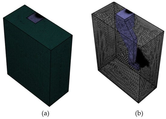
Figure 8.
Model A’s isometric mesh model viewed as (a) a solid model and (b) a wireframe model.
ANSYS Fluent meshing was also employed in models B, C, and D using the same setting as model A, but this article reveals only mesh model A in Figure 8 as an example.
To determine a suitable HAT design for the operating conditions, the T generated by hot air was investigated at 24 welding points (12 upper points and 12 lower points) depicted in Figure 9, which will be used for help analysis in Section 4, Results and Discussion.
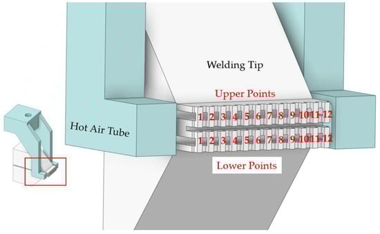
Figure 9.
The points for investigation of the temperature generated at the WT by hot air.
3.3.2. Boundary Conditions and Material Properties
Figure 10 reports the boundary conditions defined for the CFD. The inlet was defined in the top hole as blue, the outlet was assigned to surroundings marked as pink, and symmetry was used in the half-cutting plane marked as yellow. The small picture shows the defined boundary conditions viewed on the opposite side. Note that the factory operating condition is a hot air velocity at the inlet (vi) of 10 m/s, with a temperature (Ti) of 230 °C. Table 1 and Table 2 report the essential boundary conditions and material properties employed in CFD. Importantly, vi and Ti are parameters that can vary to determine the suitable operating conditions. All data in Table 2 are based on a room temperature of 24 °C.
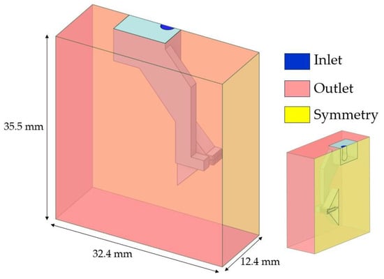
Figure 10.
The boundary conditions defined in CFD.

Table 1.
Boundary conditions.
Table 2.
Material properties.
3.3.3. Software Calculation and Settings
ANSYS Fluent v2021, a CFD commercial software, was used to investigate the T in a transient state due to the RSP. In the transient setting, the step size was 0.015 s, covering 0 to 1.5 s, 1.0 s governing 1.5 to 60 s, and the number of iterations was 20 per time step. t refers to the time from the start of supplying hot air. The turbulent model used realizable k-ε for convenience. It is better than the standard k-ε [22] and suitable for the WT and HAT geometries. The benefit of realizable k-ε is that it more accurately predicts the spreading rate of both planar and round jets. It is also likely to provide superior performance for flows involving rotation, boundary layers under strong adverse gradients, separation, and recirculation [22]; therefore, it is popular in industrial simulations. In addition, it provides accurate results compared to the experimental results after the authors had checked this in pre-simulation. The convergence absolute criteria for the continuity for velocities k and ε is 0.0001, and the energy is 10−6. The governing equations of conservation, turbulent equations for ANSYS Fluent, and forced convection are reported in [23]. After the calculation was complete, the software reported the T in the transient state for varying model designs using vi, Ti, and t as parameters. Notably, the CFD process was repeated until the CFD results were consistent with the experimental results.
4. Results and Discussion
This section includes validation, the effect of vi, Ti, and t, a suitable design for the HAT with the operating conditions, recommendations, and future work.
4.1. Validation
Figure 11 reveals the T of model A from (a) an experiment and (b) CFD using the FOC at t of 1.5 s. Note that the FOC is a vi of 10 m/s and a Ti of 230 °C. The validation is separated into qualitative and quantitative validations, explained below.
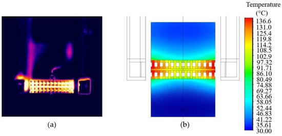
Figure 11.
The WT temperature from (a) the experiment and (b) CFD.
In a qualitative validation, in (a), the brighter it was, the higher the temperature. Comparing the figures in (a) and (b), the comparison confirmed that both results were consistent. The higher T was near the border, while the lower T was in the center.
In a quantitative validation in Figure 11, the experiment also reports that the T was in the 106.2–133.5 °C range, and the CFD reveals that it was in the 107.3–136.6 °C range. The maximum error of the CFD results is 2.3% compared to the experimental results. Figure 12 shows the T at the t from 0.3 s to 1.5 s for the experiment and CFD: (a) upper and (b) lower points. The positions in the x-axis are the welding points mentioned in Figure 9. As expected, both results were also consistent. As the t increased, the T increased. Comparing Figure 9, Figure 10, Figure 11 and Figure 12, the T near the border points 1, 2, 3, 10, 11, and 12 were higher than the T in the center points 4, 5, 6, 7, 8, and 9. As expected, the T decreased from the border to the center, consistent with Figure 11. The comparison between (a) and (b) found that the upper points had a higher T than the lower points due to the HAT design, which was consistent with what was actually observed in the experiment. The upper points had a higher T than the lower points but the difference was not greater than 4.5%.
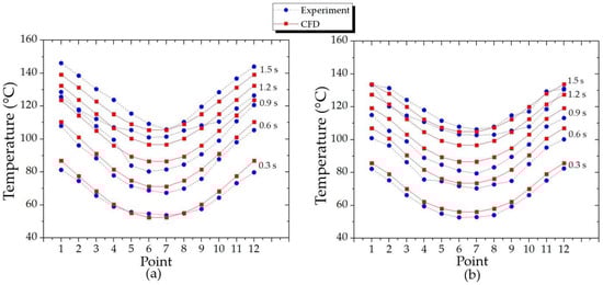
Figure 12.
The WT temperature of model A from a t of 0.3 s to 1.5 s for the (a) upper points and (b) lower points.
Accordingly, qualitative and quantitative validations confirm that this research’s CFD results and methodology are credible and suitable for the next section.
4.2. Effect of vi and Ti on the T of Model A
This section assesses the T for varying the parameters vi, Ti, and t. Using model A and a vi of 10 m/s, Figure 13 shows the T for varying Ti from 230 °C to 700 °C at a t of 1.5 s. These temperatures were the averaged values of T in the upper and lower points, since they were slightly different (below 8.5% difference, as discussed in Figure 12). As expected, the higher the Ti, the greater the T, which is consistent with the forced convection heat transfer principle governed by Equation (6). Similar to Figure 11 and Figure 12, the T at the center was lower than that at the border. The higher the Ti, the more significant the T difference. Since the RSP requires a uniform T, the lower Ti is better than the higher Ti.
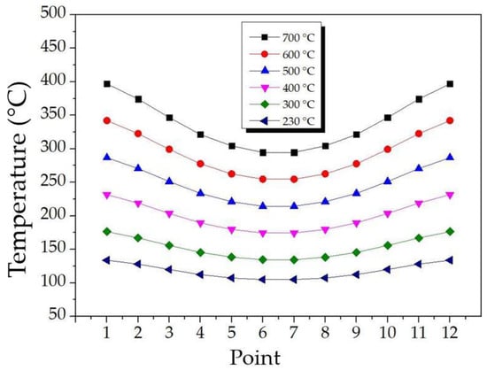
Figure 13.
The T of model A with a vi of 10 m/s at a t of 1.5 s.
Figure 14 shows the T of model A under the same conditions as in Figure 13 but with a vi varying from 10 m/s to 20 m/s and a Ti of 230 °C at t values of (a) 0.3 s, (b) 0.6 s, (c) 0.9 s, (d) 1.2 s, and (d) 1.5 s. At all times, the higher the vi, the greater the T, which is consistent with Equation (6), as expected. Similar to Figure 11, Figure 12 and Figure 13, the center points in Figure 14 had a lower T than the border. Significantly, the longer the t, the smaller the difference between the T at the center and that at the border. Accordingly, the melting should use hot air when the T is steady and even. For example, hot air can be released continuously until the temperatures in all the welding points are uniform; then the melting begins.
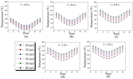
Figure 14.
The T of model A with a Ti of 230 °C at t values of (a) 0.3 s, (b) 0.6 s, (c) 0.9 s, (d) 1.2 s, and (e) 1.5 s.
Extending the hot air supply time in Figure 14e from t values of 1.5 s to 60 s, Figure 15 depicts the T at a t of 60 s as an example. As expected, the T in Figure 15 was more uniformly distributed than in Figure 2b and Figure 11, confirming that continuously releasing hot air is better. In this figure, releasing hot air for 60 s at a Ti of 230 °C and a vi of 10 m/s uniformly generated a T of about 224 °C, which is suitable for the RSP.
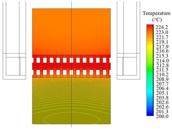
Figure 15.
The T of model A with a Ti of 230 °C at a t of 60 s.
If the solder ball is melted at 220 °C for some HDD generations, Figure 16 proposes a solution using model A to achieve 220 °C as a candidate solution for a sample requirement from HDD manufacturing. Figure 16 reveals the T using model A with a vi of 10 m/s at a t of 1.5 s for Ti values of (a) 230 °C, (b) 300 °C, (c) 400 °C, (d) 500 °C, (e) 600 °C, and (f) 700 °C. It was found that the higher the Ti, the faster the T rise, as expected. Since the requirement we set above was a rapid uniform temperature of 220 °C at the WT, cases (a), (b), (c), and (d) were not a solution; they could not generate the required T or provided T unevenly. Significantly, both (e) and (f) could generate the temperature quickly, achieving more than 220 °C within 1.5 s; therefore, both might be possible solutions. The Ti of 700 °C generated about a 12% higher T with a broader area than a Ti of 600 °C.
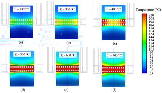
Figure 16.
The WT temperature using model A with a vi of 10 m/s at a t of 1.5 s for Ti values of (a) 230 °C, (b) 300 °C, (c) 400 °C, (d) 500 °C, (e) 600 °C, and (f) 700 °C.
However, combining the results in Figure 13, Figure 14, Figure 15 and Figure 16 implies that using model A with a very high Ti is not good, since it has a very high contrast between the T at the center and that at the border for the first 1.5 s, which is improper for the RSP.
In more in-depth analysis, supplying continuous hot air for longer than 60 s to model A with a vi of 10 m/s and a Ti of 230° (FOC) is suitable for the RSP since this FOC allows the WT to reach 220 °C with a uniform temperature. Unfortunately, model A has some disadvantages since it requires a long time to reach the melting point of solder balls and needs at least 60 s to have a uniform T. Increasing the vi reduced the time taken to reach the melting point temperature; however, model A was not supported because it generated an uneven T for a high vi. Since model A has limited practical applications because of some of its disadvantages, we had to find an alternative model for the HAT with suitable operating conditions that were better than model A. This is presented in the next section.
4.3. Suitable Design for the HAT with Operating Conditions
Figure 17 shows the CFD results of T using (a) model A, (b) model B, (c) model C, and (d) model D, i.e., employing the models in Figure 7 under the FOC during 60 s. In all models, as expected, the T increased as the t increased, which was consistent with the forced convection heat transfer principle.
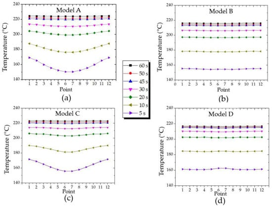
Figure 17.
The CFD results of T using the FOC during 60 s for (a) model A, (b) model B, (c) model C, and (d) model D.
Comparing the CFD results of model A (prototype) in (a) with model C in (c), both results had nearly the same trend; however, model C provided a slightly better even T distribution than model A in the first 20 s from the initiation of hot air. However, after 20 s, both results were almost the same. The difference in the first 20 s may come from the circular shape inside the HAT in model C, which allowed hot air to flow better than the square shape in model A. In the fluid dynamics principle, fluid flows in a rectangular cross section tube have higher shear stress than in a circular cross section tube [24]; consequently, model C was better than model A. The shear stress due to fluid flowing depends on the tube shape [25]. The higher the shear stress, the harder the fluid flow in the tube; therefore, fluid dynamics confirms this result. It might be explained using Equation (6) that a circular cross section has a better q than a rectangular one. Significantly, the results of models A and C also imply that if both models are implemented in the RSP, hot air should be supplied continuously until the T is uniform and constant before melting the solder balls, i.e., at least longer than 60 s.
Comparing models B and D, both results were almost identical and generated a smaller T than models A and C. Fortunately, both models provided a uniformly distributed T, which was superior to models A and C. In the heat transfer principle, models B and D lost some heat to the thin top and bottom bars, while models A and C did not. Comparing models B and D, model D provided a slightly higher T, since model D has a circular cross section tube but model B has a rectangular one. It also obeyed Equation (6), since the circular cross section has a higher q than the rectangular one.
In deep analysis, Figure 18 presents the T using the FOP for (a) model A at a t of 1.5 s, (b) model B at a t of 1.5 s, (c) model C at a t of 1.2 s, and (d) model D at a t of 1.5 s. Models A and C provided the same trend of temperature distribution, but model C required 1.2 s, while model A needed 1.5 s. As expected, the circular cross section in model C has a better q than the rectangular cross section in model A.
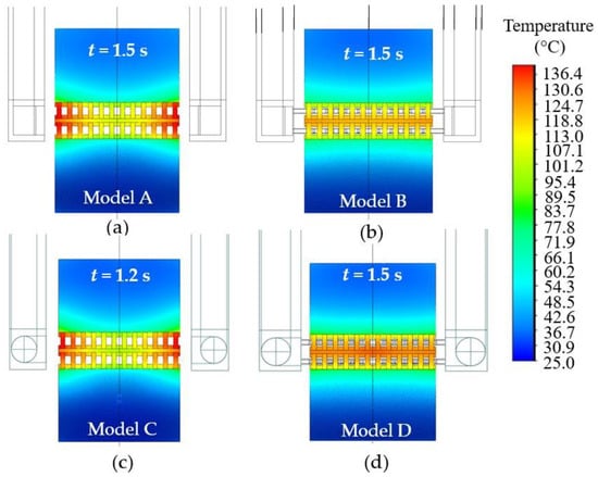
Figure 18.
The T using the FOP for (a) model A at a t of 1.5 s, (b) model B at a t of 1.5 s, (c) model C at a t of 1.2 s, and (d) model D at a t of 1.5 s.
In sum, models B and D provided uniformly distributed temperatures during the time; therefore, both are considered suitable for the RSP. Importantly, Figure 18 supports the discussion in Figure 17 and the forced convection heat transfer principle, as expected.
Figure 19 reveals the T at a t of 1.5 s for some operating conditions of (a) model B and (b) model D to find which one of these models is better.
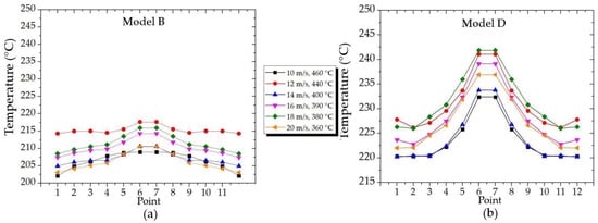
Figure 19.
The WT temperatures at a t of 1.5 s for some operating conditions of (a) model B and (b) model D.
Comparing the black lines at a vi of 10 m/s and a Ti of 460 °C, model B’s T was more uniform than model D’s. The T difference between model B’s center and border points was about 3 °C. In contrast, model D differed by about 13 °C; the center points were clearly at a higher T than the border points. Significantly, all conditions in (b) provided a strongly ununiform temperature compared to (a); hence, model B is better than model D in terms of T uniformity. Importantly, Figure 19 implies that a suitable HAT model with a proper operating condition can provide uniformly distributed T and that model B is better than model D. Next, CFD will examine an example of finding suitable operating conditions.
Figure 20 shows the T using model B with a Ti of 490 °C during 60 s for (a) a vi of 10 m/s and (b) a vi of 20 m/s. As expected, the T in (b) had a faster increase than that in (a) because a vi of 20 m/s had a higher q than a vi of 10 m/s. For example, that operating conditions in (b) increased the T from room temperature to about 375 °C within 5 s, while (a) required about 10 s. In (b), the WT needed about 30 s to reach 450 °C, but in (a), it needed 45 s. It is well known that fluid velocity is one factor that influences forced convection heat transfer capability [26], governed by Equation (6). The higher the fluid velocity, the greater the q. Therefore, model B with a vi of 20 m/s had a better q than a vi of 10 m/s, reaching the higher temperature rapidly and obeying Equation (6), as expected. However, when the supply of the hot air was longer than 60 s, the WT would start to distribute more evenly, as intended. Accordingly, supplying hot air for a long time, such as longer than 60 s, can help distribute the T evenly and assist the RSP effectively.
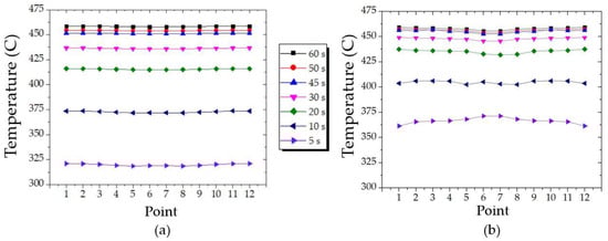
Figure 20.
The T using model B with a Ti of 490 °C during 60 s for (a) a vi of 10 m/s and (b) a vi of 20 m/s.
However, the T was uniformly distributed at all times in (a), while in (b) it slightly fluctuated and was not uniform, especially at the center points. This fluctuation in (b) may be due to a vi of 20 m/s representing hot air flowing with a high velocity into the WT; therefore, it had a higher turbulence kinetic energy (TKE). In fluid dynamics [27,28,29], the TKE measures the turbulence intensity in a fluid flow. The higher the TKE, the greater the turbulent intensity. To explain the TKE and link it to the fluid dynamics principle with Figure 20, Figure 21 reveals the TKE of hot air for (a) a vi of 10 m/s and (b) a vi of 20 m/s. Clearly, the TKE in (b) was higher than in (a); therefore, a lower vi is better. The high TKE caused the T fluctuation.
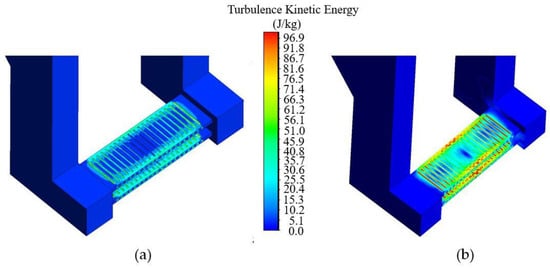
Figure 21.
The turbulence kinetic energy of hot air for (a) a vi of 10 m/s and (b) a vi of 20 m/s.
Figure 17, Figure 18, Figure 19, Figure 20 and Figure 21 imply that model B, with the operating conditions of a low Ti and slow vi, was better than others. In summary, hot air is a proper choice to assist the low-temperature RSP in achieving higher efficacy when employing suitable operating conditions. CFD is a powerful tool for determining suitable operating conditions.
4.4. Recommendations and Future Work
A critical disadvantage of using hot air is that it is improper for the high-temperature RSP, such as melting the solder balls at temperatures greater than 500 °C. The WT requires a long time and continuous high-temperature hot air flow to achieve high temperatures; therefore, using hot air for the high-temperature RSP is wasteful of energy. In addition, hot air with temperatures that are too high may disturb neighbor machines, causing malfunctions, and harm operators who operate the RSP with carelessness, leading to accidents. Accordingly, the authors recommend implementing low-temperature (below 500 °C) and low-velocity (not faster than 10 m/s) hot air and including a proper HAT design and suitable operating conditions to generate uniformly distributed temperatures in the WT for the low-temperature RSP to avoid product defects and increase efficacy.
However, if necessary, a high-temperature RSP may be suitable using a combination of supplied hot air and electric current. Referring to Figure 2, a big advantage of the RSP using an electric current is that it can rapidly generate a high temperature. Significantly, the highest temperature is mainly in the center points. In contrast, considering Figure 11, the transient hot air can generate a high temperature at the border points. Accordingly, merging Figure 2 with Figure 11, using an electric current and transient hot air to the WT and HAT in suitable operating conditions, which have been well-designed and studied, may melt the solder balls at a high temperature effectively, avoiding product defects. Since the RSP temperature induced by the electric current is based on transient thermal-electric analysis [4,5] and the RSP temperature sourced by hot air is based on CFD, developing an RSP regarding transient thermal-electric analysis and CFD as multiphysics constitutes our future work.
5. Conclusions
This article presents a feasibility study of using hot air to generate a T distributed uniformly in the RSP, one of the HDD manufacturing processes, instead of using applied current, which is conventional in the RSP but provides an ununiform T. First, the samples of the WT and HAT prototypes were designed and invented. The experiment was set in a laboratory to measure the T using the invented prototypes under the FOC, a vi of 10 m/s, and a Ti of 230 °C. Then, CFD was employed to investigate the T under the FOC and some vi and Ti operating conditions. After comparing the CFD and experimental results under the FOC, the comparison revealed the consistency between both results, confirming the credibility of the CFD results and the research methodology. The CFD results also indicated that the prototypes with the OPC provided ununiformly distributed T in the first 1.5 s from supplying hot air, which was unsuitable for the RSP. However, if hot air was continuously released for longer than 60 s, the T was more uniformly distributed than if released for short durations. In addition, if hot air was released with a hotter Ti or faster vi, the T was also more ununiformly distributed. The hotter the Ti, the more ununiformly distributed T; the faster the vi, the more ununiformly distributed T, making the prototype with the FOC unsuitable for the RSP. Accordingly, the prototype was suitable for supplying continuous hot air with a low vi and Ti. It was unsuitable for supplying hot air with a high Ti, fast vi, and transient time. Next, three additional models of the HAT were proposed to find a suitable design for the HAT with appropriate operating conditions. As expected, the CFD results revealed a difference in the uniformity of the T distribution depending on the models, obeying the forced convection heat transfer principle. Adding thin top and bottom bars to the HAT prototype in model B as a proper model improved the uniformity of the T distribution compared to the other models and was significantly superior to the prototype and consistent with the fluid dynamics principle. Lastly, the CFD results confirmed that employing the proper HAT model using hot air with a low Ti and a slow vi in the actual RSP was reasonably feasible to increase efficiency. The novel aspects of this research are the proper designs for the HAT with operating conditions that were practically employed in the actual RSP. Remarkably, hot air is a proper choice to assist the RSP in achieving a higher efficacy.
Author Contributions
Conceptualization, N.K. and J.T.; methodology, N.K. and J.T.; software, C.C. and J.T.; validation, N.K., C.C. and J.T.; formal analysis, J.T.; investigation, C.C. and J.T.; resources, J.T.; data curation, N.K.; writing—original draft preparation, J.T.; writing—review and editing, J.T.; visualization, J.T.; supervision, J.T.; project administration, J.T.; funding acquisition, J.T. All authors have read and agreed to the published version of the manuscript.
Funding
This research was funded by Research and Researchers for Industries (RRI), grant number MSD61I0097, in collaboration with Seagate Technology (Thailand) Ltd.
Data Availability Statement
Data are contained within the article.
Acknowledgments
The facilities were supported by College of Advanced Manufacturing Innovation, King Mongkut’s Institute of Technology Ladkrabang.
Conflicts of Interest
The authors declare no conflicts of interest.
Nomenclature
| CFD | computational fluid dynamics |
| FOC | factory operating condition |
| Q | flow rate (m3/s) |
| HSA | head stack assembly |
| q | heat transfer rate (W) |
| HAT | hot air tube |
| vi | hot air velocity at the inlet (m/s) |
| RSP | reflow soldering process |
| Ti | temperature of hot air at the inlet (°C) |
| t | time of supplying hot air (s) |
| TKE | turbulence kinetic energy (J/kg) |
| WT | welding tip |
| T | WT temperature (°C) |
References
- Luksamee-Arunothai, M. The structure of Thailand’s hard disk drive sector and international production networks: An input-output analysis. J. Multidiscip. Humanit. Soc. Sci. 2023, 6, 448–468. (In Thai) [Google Scholar]
- Yongpisanphob, W. Industry Outlook 2021–2023: Electronics. Available online: https://www.krungsri.com/en/research/industry/industry-outlook/hi-tech-industries/electronics/io/io-Electronics-21 (accessed on 7 August 2024). (In Thai).
- Jon, Y. Thailand’s Hard Disk Drive Industry Problem. Available online: https://www.asianometry.com/p/thailands-hard-drive-industry-problem (accessed on 8 August 2024).
- Thongsri, J. Transient Thermal-Electric Simulation and Experiment of Heat Transfer in Welding Tip for Reflow Soldering Process. Math. Probl. Eng. 2018, 2018, 4539054. [Google Scholar] [CrossRef]
- Thongsri, J.; Jansaengsuk, T. A Development of Welding Tip for the Reflow Soldering Process Based on Multiphysics. Processes 2022, 10, 2191. [Google Scholar] [CrossRef]
- Kimaporn, N.; Samakkarn, C.; Thongsri, J. Multiphysics to Investigate the Thermal and Mechanical Responses in Hard Disk Drive Components due to the Reflow Soldering Process. Processes 2024, 12, 2029. [Google Scholar] [CrossRef]
- Llés, B.; Krammer, O.; Géczy, A. Reflow Soldering: Apparatus and Heat Transfer Processes, 1st ed.; Elsevier: Amsterdam, The Netherlands, 2020. [Google Scholar]
- Lam, T.L. Low-Cost Non Contact PCBs Temperature Monitoring and Control in a How Air Reflow Process Based on Multiple Thermocouples Data Fusion. IEEE Access 2021, 9, 123566–123574. [Google Scholar] [CrossRef]
- Hong, W.S.; Kin, M.S.; Kim, M. MLCC Solder Joint Property with Vacuum and Hot Air Reflow Soldering Processes. J. Weld. Join. 2021, 39, 349–358. [Google Scholar] [CrossRef]
- Sweatman, K. Hot Air Solder Leveling in the Lead-Free Era. Glob. SMT Packag. 2009, 10–18. [Google Scholar]
- Molhanec, M. Study of Solder Spreadability at Different Soldering Conditions Using Factorial Experiments. In Proceedings of the ISSE 2019 42nd International Spring Seminar on Electronics Technology (ISSE), Wroclaw, Poland, 15–19 May 2019; pp. 1–4. [Google Scholar] [CrossRef]
- Dušek, K.; Veselý, P.; Bušek, D.; Froš, D.; Králová, I.; Klimtová, M.; Pilnaj, D.; Uřičář, J.; Plachý, Z.; Sorokina, K.; et al. Influence of Reflow Temperature Profile on the Intermetallic Layers Thickness at Different Surface Finishes. In Proceedings of the ISSE 2024 47th International Spring Seminar on Electronics Technology, Prague, Czech Republic, 15–19 May 2024; pp. 1–4. [Google Scholar] [CrossRef]
- Deng, S.S.; Hwang, S.J.; Lee, H.H. Temperature Prediction for System in Package Assembly during the Reflow Soldering Process. Int. J. Heat Mass Transf. 2016, 98, 1–9. [Google Scholar] [CrossRef]
- Ran, L.; Chen, D.; Chen, C.; Gong, Y. Optimization Method for How Air Reflow Soldering Process Based on Robus Design. Processes 2023, 11, 2716. [Google Scholar] [CrossRef]
- Srivalli, C.; Abdullah, M.Z.; Khor, C.Y. Numerical Investigations on the Effects of Different Cooling Periods in Reflow-Soldering Process. Heat Mass Transf. 2015, 51, 1413–1423. [Google Scholar] [CrossRef]
- Ferreira, A.C.; Teixeira, S.F.C.F.; Oliverira, R.F.; Rodrigues, N.J.; Teixeira, J.C.F.; Soares, D. CFD Modeling the Cooling Stage of Reflow Soldering Process. In Proceedings of the ASME 2016 International Mechanical Engineering Congress and Exposition, Pheonix, AZ, USA, 11–17 November 2016. [Google Scholar]
- Zheng, Y.; Fang, J.; Wei, L.; Shen, H.; Gong, Y. Shape Prediction of the BGA solder Joint in Hot Air Air Flow Soldering Based on CFD. In Proceedings of the MEMAT 2022; 2nd International Conference on Mechanical Engineering, Intelligent Manufacturing and Automation Technology, Guilin, China, 7–9 January 2022; pp. 1–5. [Google Scholar]
- Bozsóki, I.; Géczy, A.; Illés, B. Overview of Different Approaches in Numerical Modelling of Reflow Soldering Applications. Energies 2023, 16, 5856. [Google Scholar] [CrossRef]
- Storey, B.D. Fluid Dynamics and Heat Transfer: An Introduction to the Fundamentals. Available online: http://faculty.olin.edu/bstorey/transport.pdf (accessed on 10 August 2024).
- ANSYS, Inc. Module 05: Mesh Quality & Advanced Topics. In Introduction to ANSYS Meshing; ANSYS Inc: Canonsburg, PA. USA, 2016. [Google Scholar]
- Matsson, J.E. An Introduction to ANSYS Fluent 2024; SDC Publications: Mission, KS, USA, 2024. [Google Scholar]
- Shaheed, R.; Mohammadian, A.; Gildeh, H.K. A Comparison of Standard k-ε and Realizable k-ε turbulence models in curved and confluent channels. Environ. Fluid Mech. 2019, 19, 543–568. [Google Scholar] [CrossRef]
- ANSYS Inc. Chapter 4 Turbulence. In Ansys Fluent 17.1, User’s Guide; Ansys Inc.: Canonsburg, PA, USA, 2016. [Google Scholar]
- Shahriar, M.; Monir, M.I.; Deb, U.K. Comparative Analysis of Hydrodynamics Behavior of Microalgae Suspension Flow in Circular, Square, and Hexagonal Shape Photo Bioreactors. Am. J. Comput. Math. 2016, 6, 320–355. [Google Scholar] [CrossRef][Green Version]
- Hoogenboom, P.C.J.; Spann, R. Shear Stiffness and Maximum Shear Stress of Tabular Members. In Proceedings of the 15th International Offshore and Polar Engineering Conference, Seoul, Republic of Korea, 19–24 June 2005. [Google Scholar]
- Parlak, F.; Sertkaya, A.A. Experimental Investigation of Forced Convection Heat Transfer of Heat Exchanger with Different Pin Geometries in in-line and Staggered Design. Int. J. Heat Mass Tranf. 2024, 231, 125892. [Google Scholar] [CrossRef]
- Bailly, C.; Comte-Bellot, G. Turbulence. Chapter 9: Turbulence Model; Springer: Berlin/Heidelberg, Germany, 2015. [Google Scholar]
- ANSYS Inc. Turbulence, Fluent Theory Guide 17.1; ANSYS Inc.: Sountpointe, FL, USA, 2016. [Google Scholar]
- Faizal, W.M.; Khor, C.Y.; Yaakob, M.N.C.; Ghazali, N.N.N.; Zainon, M.Z.; Ibrahim, N.B.; Razi, R.M. Turbulent Kinetic Energy of Flow during Inhale and Exhale to Characterize the Severity of Obstructive Sleep Apnea Patient. Comput. Model. Eng. Sci. 2023, 136, 43–61. [Google Scholar] [CrossRef]


Disclaimer/Publisher’s Note: The statements, opinions and data contained in all publications are solely those of the individual author(s) and contributor(s) and not of MDPI and/or the editor(s). MDPI and/or the editor(s) disclaim responsibility for any injury to people or property resulting from any ideas, methods, instructions or products referred to in the content. |
© 2024 by the authors. Licensee MDPI, Basel, Switzerland. This article is an open access article distributed under the terms and conditions of the Creative Commons Attribution (CC BY) license (https://creativecommons.org/licenses/by/4.0/).