
Enhanced Transverse Dispersion in 3D-Printed Logpile Structures: A Comparative Analysis of Stacking Configurations

 , and
, and 
Abstract
:1. Introduction
2. Methods
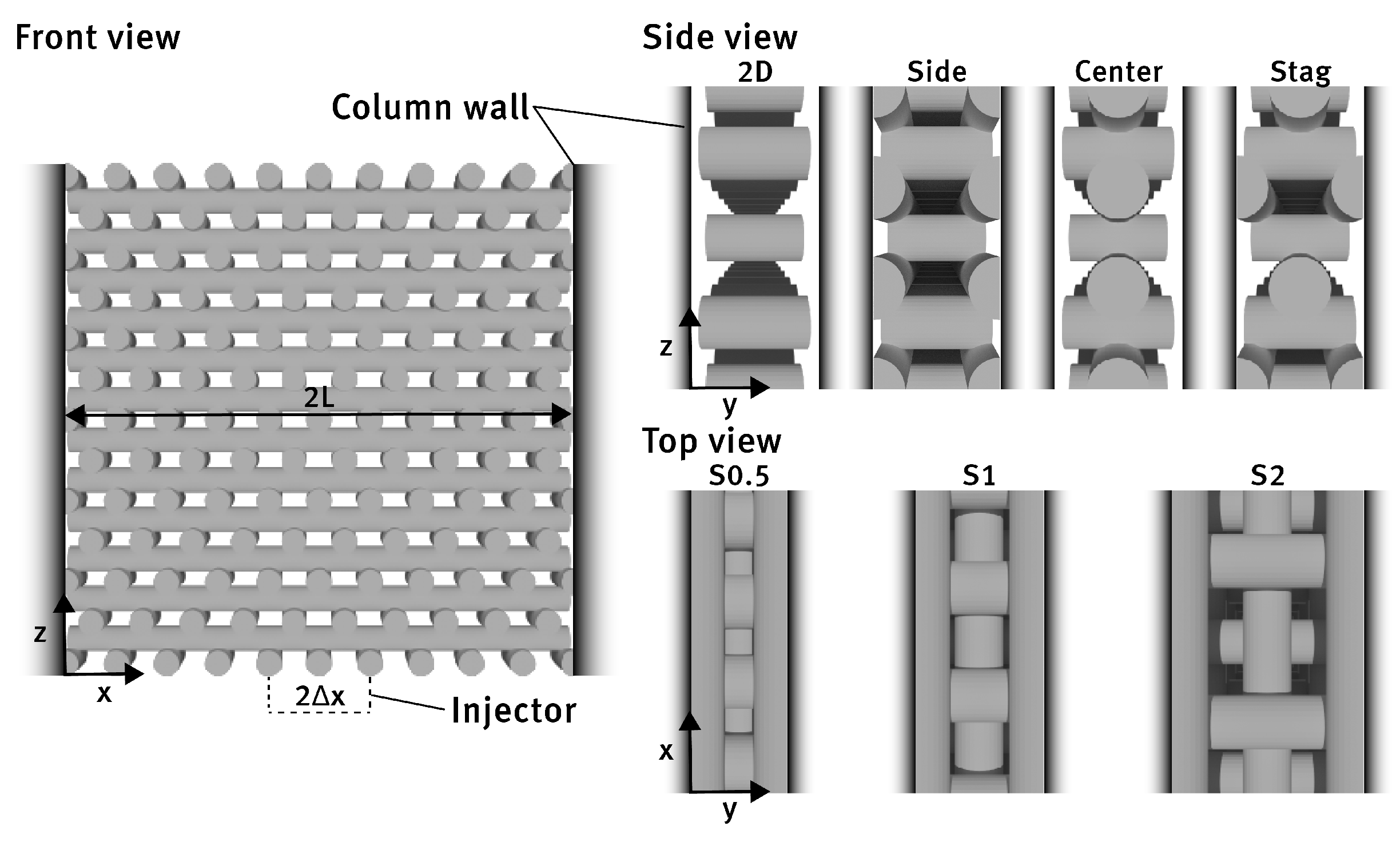
2.1. Geometries
2.2. Simulation Setup
2.3. Data Evaluation
- The system is at steady state and temporal fluctuations due to vortex shedding are averaged. The resolution of averaging for representative estimates is discussed in Section 2.4.
- A uniform axial velocity profile is assumed from the reactor scale perspective. The influence of transverse velocity profiles is not considered explicitly, as their effect is incorporated into the dispersion coefficient. It is assumed that the dispersion coefficient remains constant throughout the structure. This assumption is valid in the absence of hydrodynamic entrance effects, which is discussed in Section 2.5.
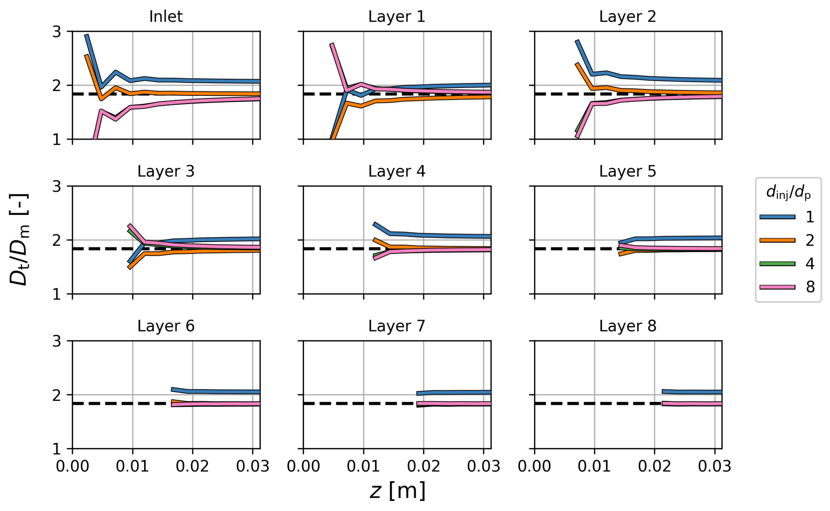
- The concentration profiles in the secondary transverse direction (the y-direction) were condensed into a single concentration profile in the primary transverse direction (the x-direction). This is justified since the tracer is injected along the entire length of secondary transverse axis. Furthermore, it was observed that concentration gradients along this axis were negligible compared to the profiles obtained along the x-axis.
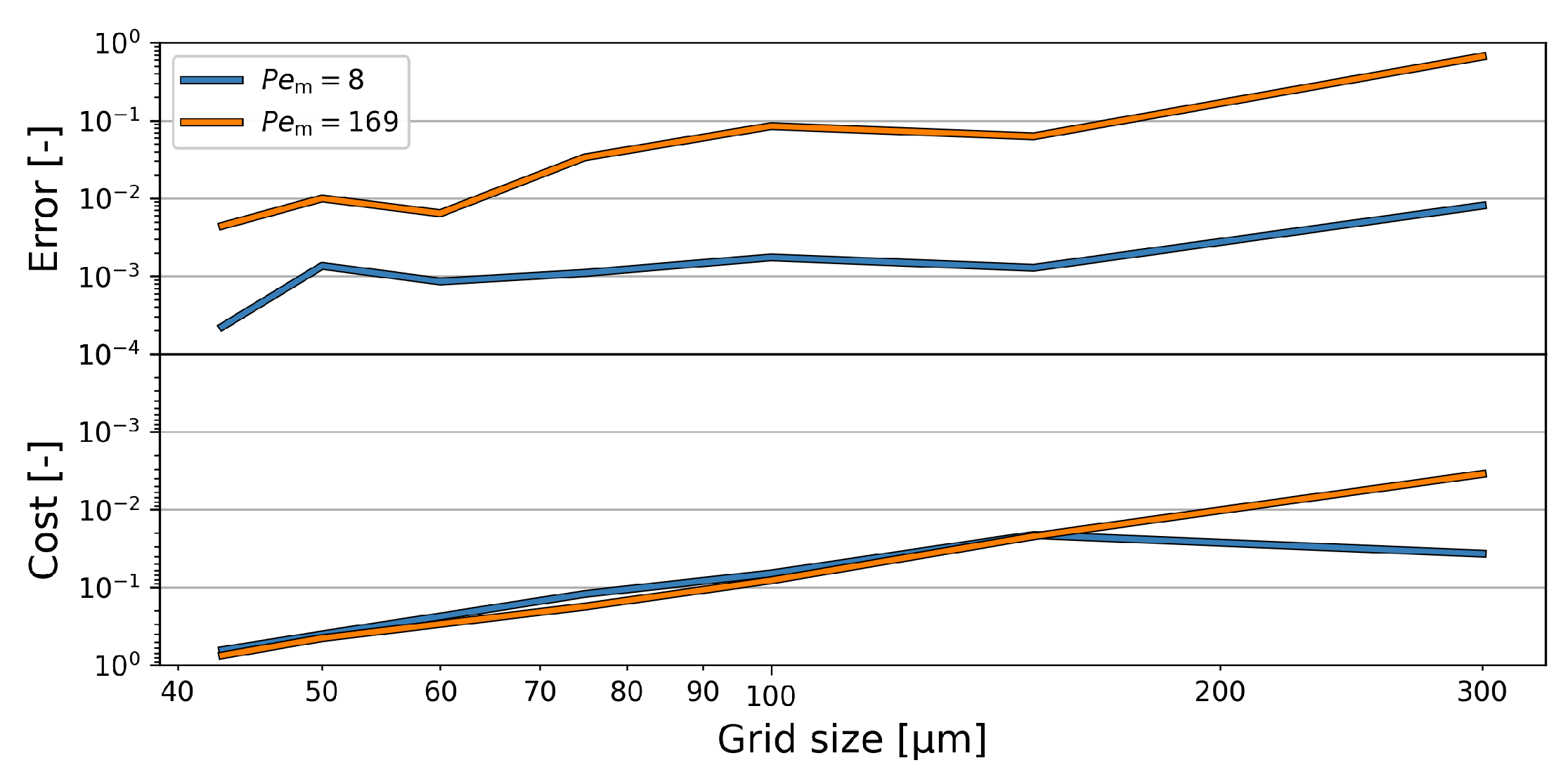
2.4. Steady State and Time-Averaging
2.5. Hydrodynamic Entrance Effects
3. Results
4. Conclusions
Author Contributions
Funding
Data Availability Statement
Conflicts of Interest
Nomenclature
| Symbol | Representation | Unit |
| C | Concentration | mol m−3 |
| Drag coefficient | - | |
| D | Dispersion coefficient | m2 s−1 |
| d | Diameter | |
| h | Axial length | |
| k | Turbulent kinetic energy | m2 s−2 |
| L | Half column width | |
| N | Number of data points | - |
| n | Counting variable | - |
| Péclet number | - | |
| p | Pressure | |
| Reynolds number | - | |
| t | Time | |
| Dimensionless time | - | |
| U | Superficial velocity | m s−1 |
| Velocity vector | m s−1 | |
| u | Interstitial velocity | m s−1 |
| x | Primary transverse coordinate | |
| Y | Mass fraction | - |
| y | Secondary transverse coordinate | |
| z | Axial coordinate | |
| Fitted coefficient | - | |
| Fitted coefficient | - | |
| Pressure drop | ||
| Half injection width | ||
| Porosity | - | |
| Dynamic viscosity | ||
| Density | kg m−3 | |
| Standard deviation | ||
| Stress tensor | ||
| Tortuosity | - | |
| Specific dissipation rate | s−1 | |
| Subscript | Representation | |
| 0 | Reference | |
| f | Fluid | |
| inj | Injection | |
| m | Molecular | |
| p | Particle | |
| t | Transverse |
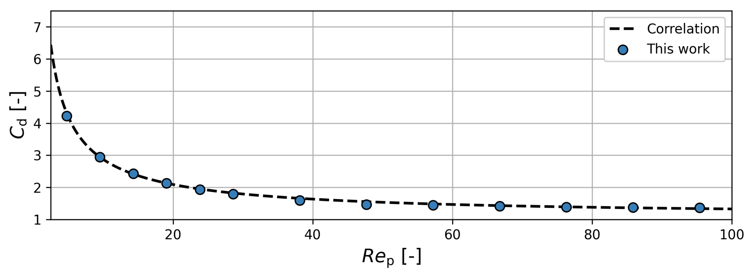
Appendix A. Solver Validation: Drag Coefficient
Appendix B. Validity of Laminar Flow Regime
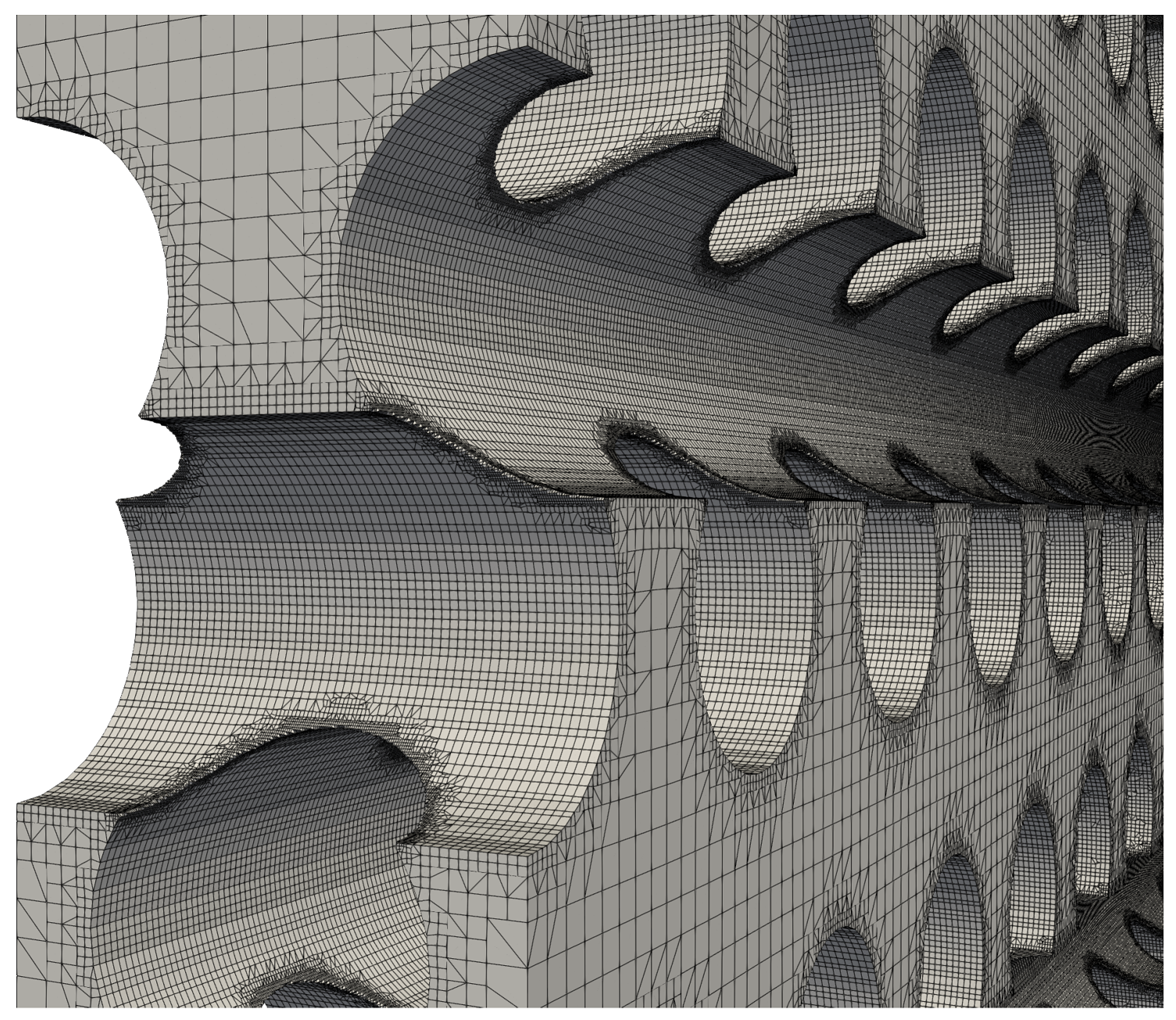
Appendix C. Mesh Refinement Visualization
References
- Lerou, J.J.; Froment, G.F. Velocity, temperature and conversion profiles in fixed bed catalytic reactors. Chem. Eng. Sci. 1977, 32, 853–861. [Google Scholar] [CrossRef]
- Kapteijn, F.; Moulijn, J.A. Structured catalysts and reactors—Perspectives for demanding applications. Catal. Today 2020, 383, 5–14. [Google Scholar] [CrossRef]
- Griesinger, A.; Spindler, K.; Hahne, E. Measurements and theoretical modelling of the effective thermal conductivity of zeolites. Int. J. Heat Mass Transf. 1999, 42, 4363–4374. [Google Scholar] [CrossRef]
- Miscke, R.A.; Smith, J.M. Thermal conductivity of alumina catalyst pellets. Ind. Eng. Chem. Fundam. 1962, 1, 288–292. [Google Scholar] [CrossRef]
- Jayachandran, S.; Reddy, K.S. Estimation of effective thermal conductivity of packed beds incorporating effects of primary and secondary parameters. Therm. Sci. Eng. Prog. 2019, 11, 392–408. [Google Scholar] [CrossRef]
- Dixon, A.G. Fixed bed catalytic reactor modelling—The radial heat transfer problem. Can. J. Chem. Eng. 2012, 90, 507–527. [Google Scholar] [CrossRef]
- Delgado, J.M.P.Q. A critical review of dispersion in packed beds. Heat Mass Transf. 2006, 42, 279–310. [Google Scholar] [CrossRef]
- Shinnar, R.; Doyle, F.J.; Budman, H.M.; Morari, M. Design considerations for tubular reactors with highly exothermic reactions. AIChE J. 1992, 38, 1729–1743. [Google Scholar] [CrossRef]
- Stankiewicz, A. Advances in modelling and design of multitubular fixed-bed reactors. Chem. Eng. Technol. 1989, 12, 113–130. [Google Scholar] [CrossRef]
- Wehinger, G.D. Improving the radial heat transport and heat distribution in catalytic gas-solid reactors. Chem. Eng. Process. Process Intensif. 2022, 177, 108996. [Google Scholar] [CrossRef]
- Rosseau, L.R.S.; Middelkoop, V.; Willemsen, J.A.M.; Roghair, I.; van Sint Annaland, M. Review on additive manufacturing of catalysts and sorbents and the potential for process intensification. Front. Chem. Eng. 2022, 4, 834547. [Google Scholar] [CrossRef]
- Lawson, S.; Adebayo, B.; Robinson, C.; Al-Naddaf, Q.; Rownaghi, A.; Rezaei, F. The effects of cell density and intrinsic porosity on structural properties and adsorption kinetics in 3D-printed zeolite monoliths. Chem. Eng. Sci. 2020, 218, 115564. [Google Scholar] [CrossRef]
- Huang, K.; Elsayed, H.; Franchin, G.; Colombo, P. Additive manufacturing of SiOC scaffolds with tunable structure-performance relationship. J. Eur. Ceram. Soc. 2021, 41, 7552–7559. [Google Scholar] [CrossRef]
- Lawson, S.; Li, X.; Thakkar, H.; Rownaghi, A.A.; Rezaei, F. Recent Advances in 3D Printing of Structured Materials for Adsorption and Catalysis Applications. Chem. Rev. 2021, 121, 6246–6291. [Google Scholar] [CrossRef] [PubMed]
- Lefevere, J.; Mullens, S.; Meynen, V. The impact of formulation and 3D-printing on the catalytic properties of ZSM-5 zeolite. Chem. Eng. J. 2018, 349, 260–268. [Google Scholar] [CrossRef]
- Beck, V.A.; Ivanovskaya, A.N.; Chandrasekaran, S.; Forien, J.B.; Baker, S.E.; Duoss, E.B.; Worsley, M.A. Inertially enhanced mass transport using 3D-printed porous flow-through electrodes with periodic lattice structures. Proc. Natl. Acad. Sci. USA 2021, 118, e2025562118. [Google Scholar] [CrossRef] [PubMed]
- Buyruk, E. Numerical study of heat transfer characteristics on tandem cylinders, inline and staggered tube banks in cross-flow of air. Int. Commun. Heat Mass Transf. 2002, 29, 355–366. [Google Scholar] [CrossRef]
- Hishikar, P.; Gaba, V.K.; Dhiman, S.K.; Tiwari, A.K. Heat transfer analysis of nine cylinders arranged inline and staggered at subcritical Reynolds number. Numer. Heat Transf. A 2024, in press. [Google Scholar] [CrossRef]
- Rosseau, L.R.S.; Schinkel, M.A.M.R.; Roghair, I.; van Sint Annaland, M. Experimental Quantification of Gas Dispersion in 3D-Printed Logpile Structures Using a Noninvasive Infrared Transmission Technique. ACS Eng. Au 2022, 2, 236–247. [Google Scholar] [CrossRef]
- Greenshields, C.; Weller, H. Notes on Computational Fluid Dynamics: General Principles; CFD Direct Ltd: Reading, UK, 2022. [Google Scholar]
- Crank, J. The Mathematics of Diffusion; Oxford University Press: Oxford, UK, 1975. [Google Scholar]
- Li, T.; Deen, N.G.; Kuipers, J.A. Numerical investigation of hydrodynamics and mass transfer for in-line fiber arrays in laminar cross-flow at low Reynolds numbers. Chem. Eng. Sci. 2005, 60, 1837–1847. [Google Scholar] [CrossRef]
- Gnielinski, V. Heat transfer in cross-flow around single rows of tubes and through tube bundles. In VDI Heat Atlas; Springer: Berlin/Heidelberg, Germany, 2010; pp. 725–730. [Google Scholar]
- Delgado, J.M.P.Q. Longitudinal and transverse dispersion in porous media. Chem. Eng. Res. Des. 2007, 85, 1245–1252. [Google Scholar] [CrossRef]
- Ahn, D.; Kweon, J.H.; Kwon, S.; Song, J.; Lee, S. Representation of surface roughness in fused deposition modeling. J. Mater. Process. Technol. 2009, 209, 5593–5600. [Google Scholar] [CrossRef]
- Puckert, D.K.; Rist, U. Experiments on critical Reynolds number and global instability in roughness-induced laminar–turbulent transition. J. Fluid Mech. 2018, 844, 878–904. [Google Scholar] [CrossRef]
- Kandlikar, S.G.; Joshi, S.; Tian, S. Effect of Surface Roughness on Heat Transfer and Fluid Flow Characteristics at Low Reynolds Numbers in Small Diameter Tubes. Heat Transf. Eng. 2010, 24, 4–16. [Google Scholar] [CrossRef]
- Brackbill, T.P.; Kandlikar, S.G. Effect of Sawtooth Roughness on Pressure Drop and Turbulent Transition in Microchannels. Heat Transf. Eng. 2007, 28, 662–669. [Google Scholar] [CrossRef]
- Buj-Corral, I.; Domínguez-Fernández, A.; Gómez-Gejo, A. Effect of Printing Parameters on Dimensional Error and Surface Roughness Obtained in Direct Ink Writing (DIW) Processes. Materials 2020, 13, 2157. [Google Scholar] [CrossRef]
- Hossain, S.S.; Lu, K. Recent progress of alumina ceramics by direct ink writing: Ink design, printing and post-processing. Ceram. Int. 2023, 49, 10199–10212. [Google Scholar] [CrossRef]
- Tanino, Y.; Nepf, H.M. Lateral dispersion in random cylinder arrays at high Reynolds number. J. Fluid Mech. 2008, 600, 339–371. [Google Scholar] [CrossRef]
- Franke, R.; Rodi, W.; Schönung, B. Numerical calculation of laminar vortex-shedding flow past cylinders. J. Wind Eng. Ind. Aerod. 1990, 35, 237–257. [Google Scholar] [CrossRef]
- Khalifa, Z.; Pocher, L.; Tilton, N. Regimes of flow through cylinder arrays subject to steady pressure gradients. Int. J. Heat Mass Transf. 2020, 159, 120072. [Google Scholar] [CrossRef]
- Vanapalli, S.; ter Brake, H.J.M.; Jansen, H.V.; Burger, J.F.; Holland, H.J.; Veenstra, T.T.; Elwenspoek, M.C. Pressure drop of laminar gas flows in a microchannel containing various pillar matrices. J. Micromech. Microeng. 2007, 17, 1381–1386. [Google Scholar] [CrossRef]
- Rosseau, L.R.S.; Jansen, J.T.A.; Roghair, I.; van Sint Annaland, M. Favorable trade-off between heat transfer and pressure drop in 3D printed baffled logpile catalyst structures. Chem. Eng. Res. Des. 2023, 196, 214–234. [Google Scholar] [CrossRef]
- Cheng, N.S. Calculation of Drag Coefficient for Arrays of Emergent Circular Cylinders with Pseudofluid Model. J. Hydraul. Eng. 2013, 139, 602–611. [Google Scholar] [CrossRef]
- Tritton, D.J. Experiments on the flow past a circular cylinder at low Reynolds numbers. J. Fluid Mech. 1959, 6, 547–567. [Google Scholar] [CrossRef]
- Qu, L.; Norberg, C.; Davidson, L.; Peng, S.H.; Wang, F. Quantitative numerical analysis of flow past a circular cylinder at Reynolds number between 50 and 200. J. Fluids Struct. 2013, 39, 347–370. [Google Scholar] [CrossRef]


| S0.5 | S1 | S2 | |
|---|---|---|---|
| 2D | 67.5% | 75.6% | 83.7% |
| 3D—fixed | 47.1% | 54.7% | 62.2% |
| 3D—scaled | 40.3% | 54.7% | 69.4% |
| Structure | COV [-] | [Pa] |
|---|---|---|
| S0.5 | ||
| S1 | ||
| S2 | ||
| S0.5 | 4.87 | |
| S1 | 2.62 | |
| S2 | 1.28 |
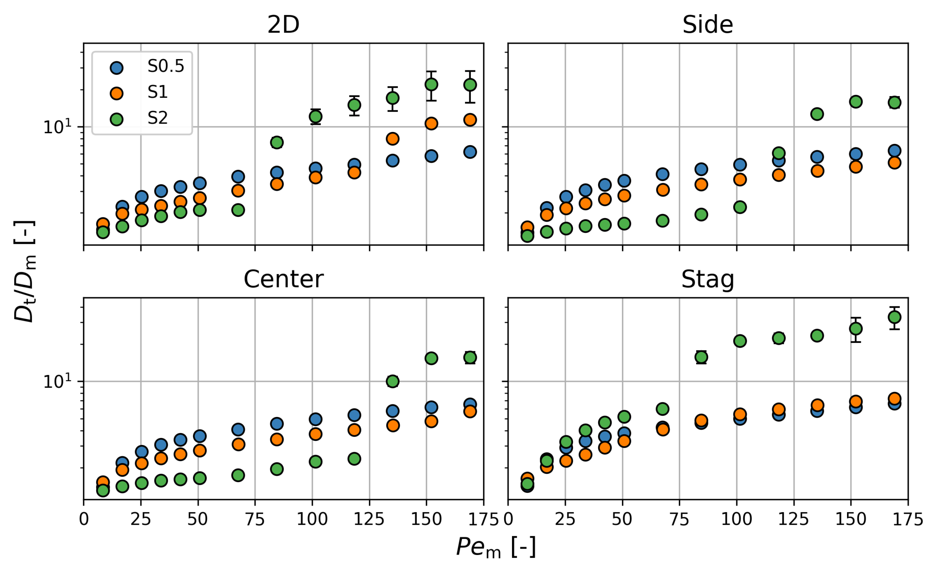
| Stacking Configuration | MAPE | ||
|---|---|---|---|
| 2D | 11.5 | 0.41 | 8.9% |
| side | 61.9 | 0.58 | 6.4% |
| center | 64.4 | 0.60 | 6.5% |
| stag | 49.8 | 0.47 | 10% |
Disclaimer/Publisher’s Note: The statements, opinions and data contained in all publications are solely those of the individual author(s) and contributor(s) and not of MDPI and/or the editor(s). MDPI and/or the editor(s) disclaim responsibility for any injury to people or property resulting from any ideas, methods, instructions or products referred to in the content. |
© 2024 by the authors. Licensee MDPI, Basel, Switzerland. This article is an open access article distributed under the terms and conditions of the Creative Commons Attribution (CC BY) license (https://creativecommons.org/licenses/by/4.0/).
Share and Cite
Rosseau, L.R.S.; van Aarle, M.A.A.; van Laer, E.; Roghair, I.; van Sint Annaland, M. Enhanced Transverse Dispersion in 3D-Printed Logpile Structures: A Comparative Analysis of Stacking Configurations. Processes 2024, 12, 2151. https://doi.org/10.3390/pr12102151
Rosseau LRS, van Aarle MAA, van Laer E, Roghair I, van Sint Annaland M. Enhanced Transverse Dispersion in 3D-Printed Logpile Structures: A Comparative Analysis of Stacking Configurations. Processes. 2024; 12(10):2151. https://doi.org/10.3390/pr12102151
Chicago/Turabian StyleRosseau, Leon R. S., Martijn A. A. van Aarle, Egbert van Laer, Ivo Roghair, and Martin van Sint Annaland. 2024. "Enhanced Transverse Dispersion in 3D-Printed Logpile Structures: A Comparative Analysis of Stacking Configurations" Processes 12, no. 10: 2151. https://doi.org/10.3390/pr12102151