Research on Dimension Reduction Method for Combustion Chamber Structure Parameters of Wankel Engine Based on Active Subspace

Abstract

The combustion chamber structure of a rotary engine involves a combination of interacting parameters that are simultaneously constrained by engine size, compression ratio, machining, and strength. It is more difficult to study the weight of the effect of the combustion chamber structure on the engine performance using traditional linear methods, and it is not possible to find the combination of structural parameters that has the greatest effect on the engine performance under the constraints. This makes it impossible to optimize the combustion chamber structure of a rotary engine by focusing on important structural parameters; it can only be optimized based on all structural parameters. In order to solve the above problems, this paper proposes a method of dimensionality reduction for the structural parameters of a combustion chamber based on active subspace and combining a probability box and the EDF (Empirical Distribution Function). This method uses engine performance indexes such as explosion pressure, maximum cylinder temperature, and indicated average effective pressure as the influence proportion analysis targets and quantitatively analyzes the influence proportion of combustion chamber structure parameters on engine performance. Eight main structural parameters with an influence of more than 85% on the engine performance indexes were obtained, on the basis of which three important structural parameters with an influence of more than 45% on the engine performance indexes and three adjustable structural parameters with an influence of less than 15% on the engine performance indexes were determined. This quantitative analysis work provides an optimization direction for the further optimization of the combustion chamber structure in the future.

1. Introduction

As a reliable power system, the internal combustion engine is widely used in many fields. Nowadays, inexpensive and reliable small engines are widely used as propulsion or auxiliary systems in motorcycles, all-terrain vehicles, boats, and small airplanes [1,2]. Although small piston engines are heavily used, they are less efficient compared to large piston engines [3,4,5]. And unlike a four-stroke reciprocating engine, where the piston stops briefly four times per cycle as the direction of motion changes, the moving parts of a rotary engine maintain a continuous, unidirectional rotary motion, which results in smoother work and less vibration [6,7,8]. At the same time, the rotary engine also has the advantages of higher power density, simple design, compact structure, and light weight [9,10,11]. These advantages make rotary engines strong competitors to reciprocating piston engines in areas such as supercharged vehicles and small unmanned aerial vehicles [12,13,14].

However, due to the narrow and flat combustion chamber shape, high surface area, and low compression ratio, it is difficult for rotary engines to achieve the fuel economy of reciprocating engines [15,16,17,18], which restricts the application of rotary engines in various fields [19,20]. In order to improve fuel economy and optimize rotary engine performance, scholars in various countries have conducted a series of investigations on engine structure [21,22,23,24]. For example, Kuo et al. investigated the effect of rotor profile on the compression flow of an engine by numerical analysis and found that increasing the shape factor K can benefit the compression efficiency and mixture formation [25]. Tartakovsky et al. started with the in-cylinder flow field and improved the engine performance by optimizing the rotor combustion chamber structure [26]. Jeng et al. further took the degree of mixing between fuel and air as the entry point and improved the engine performance by optimizing the rotor combustion chamber structure [27]. Wei et al. noticed that the position of the rotor combustion chamber has an effect on flame propagation and improved the engine performance by optimizing the rotor combustion chamber position [28,29,30]. Shi Cheng et al. investigated the role of turbulent blade position in the combustion process of a rotary engine and found that the closer the turbulent blade is to the spark plug chamber, the higher the turbulence velocity and turbulence dissipation rate are in the spark region. It was shown that the combustion rate of the mixture in the combustion chamber with a turbulent blade was accelerated, and it was able to exhibit better combustion characteristics and emission performance [31,32,33,34]. Zeng et al. [35] studied the influence of a turbulent blade on flow and combustion performance in the combustion chamber by numerically analyzing the total pressure loss, combustion efficiency, in-cylinder flow, and cylinder temperature changes of the combustion chamber under different spoiler structure parameters. It was found that adding a turbulent blade to the combustion chamber is beneficial to stabilize the combustion and gas mixing, which can further improve the combustion efficiency, improve the outlet temperature distribution, and reduce the pollutant emissions.

However, the above study only focuses on the influence of a certain structural parameter on engine performance and does not quantitatively analyze the proportions of the influence of all combustion chamber structural parameters on engine performance. This leads to the problem of dimensional catastrophe due to too many parameters to be optimized and the problem of not being able to determine the direction of optimization due to unclear parameter optimization priorities when optimizing the combustion chamber structure. Aiming at the combustion chamber structure, which is a complex physical system involving multiple disciplines and multidimensional uncertainties, domestic and foreign scholars have proposed a number of methods for dimensionality reduction. Among them, the gradient solver represented by Sensitivity Analysis (SA) [36] achieves dimensionality reduction by determining the magnitude of the influence of design and state variables on the objective or constraint functions and then filtering out the inputs with less influence. Linear projection methods represented by Classical Multidimensional Scaling (MDS) [37], Principal Component Analysis (PCA) [38], Linear Discriminant Analysis (LDA) [39], and Random Projection (RP) [40] complete the dimensionality reduction and sensitivity analysis processing by mapping the high-latitude problem to the low-latitude space. However, the above methods are not ideal for the dimensionality reduction and quantification of complex nonlinear problems. In this case, a nonlinear method is needed for dimensionality reduction. Common nonlinear methods include Kernel Principal Component Analysis (KPCA) [41], Local Linear Embedding (LLE) [42], Hessian Locally Linear Embedding (HLLE) [43], Laplacian Eigenmaps (LE) [44], and so on. However, the above methods are less computationally efficient in the face of complex, high-dimensional problems, especially in the face of mixed uncertainty problems, and are more sensitive to the selection of samples required for dimensionality reduction, which leads to the limited application of the above methods. In order to solve the problem of mixed uncertainty dimensionality reduction for complex systems, Paul et al. proposed a special dimensionality reduction structure, the Active Subspace (AS), in 2013 [45]. An AS is a low-dimensional action subspace defined by the sensitive directions of the input space, along which input perturbations maximize the effect on the output. By identifying and utilizing the AS, the dimensionality reduction process can be accelerated while ensuring the analysis accuracy.

In this paper, on the basis of previous research, based on the AS, by combining the probability box with the interval variable Empirical Distribution Function (EDF) [46,47], a method of dimensionality reduction of the structural parameters of the combustion chamber of a rotary engine is proposed. A total of 14 combustion chamber structural parameters, including the turbulent blade, were subjected to eigenvalue estimation and dimensionality reduction, and the weights of the effects of different structural parameters on the maximum cylinder pressure, the maximum cylinder temperature, and the average effective pressure were obtained. Eight main structural parameters, including the angle θ1 between the bottom edge of the middle part of the combustion chamber and the Y-Z plane were further obtained, and the influence of these structural parameters on the engine performance indexes accounted for more than 85%. Three important structural parameters, including the angle θ2 between the bottom edge of the rear part of the combustion chamber and the Y-Z plane, were obtained on this basis, and the influence of these structural parameters on the engine performance indexes accounted for more than 45%. Three adjustable structural parameters, including the length l of the bottom edge of the front of the combustion chamber, were obtained. The influence of these three structural parameters on the engine performance index accounts for a relatively small percentage, below 15%, but their influence on the compression ratio and other structural requirements is larger and can be adjusted according to the compression ratio, process, and strength requirements after determining the main structural parameters. This quantitative analysis work provides an optimization direction and theoretical support for the further optimization of the combustion chamber structure in the future. At the same time, this study provides a reference basis for eigenvalue estimation and dimension reduction methods for multidimensional complex engineering problems.

2. Uncertainty Analysis of Combustion Chamber Structure Parameters

In practical engineering, the probability distribution is divided into random uncertainty and cognitive uncertainty [48,49]. The former has a known distribution function, and the latter lacks such a function.

This study investigates how structural parameter uncertainty in the combustion chamber impacts single-cylinder gasoline Wankel engine performance.

Table 1. Rotor engine structure parameters.

Parameter	Value
Creation radius (mm)	60
Eccentricity (mm)	10
Rotor width (mm)	42
Translational distance (mm)	1.45
Speed (r/min)	8000
Single cylinder volume (cc)	133
Compression ratio	10
Ignition advance angle	30° BTDC
Ignition source	Single spark plug
Fuel type	Gasoline
Jet strategy	Pre-mixed intake duct
Air–fuel ratio	1
Ignition diameter (mm)	8
Ignition energy (J)	0.08
Engine power (kw)	12.3
Torque (N.m)	15.66
Oil consumption (g/kw·h)	402.3

lists the engine’s structural parameters.

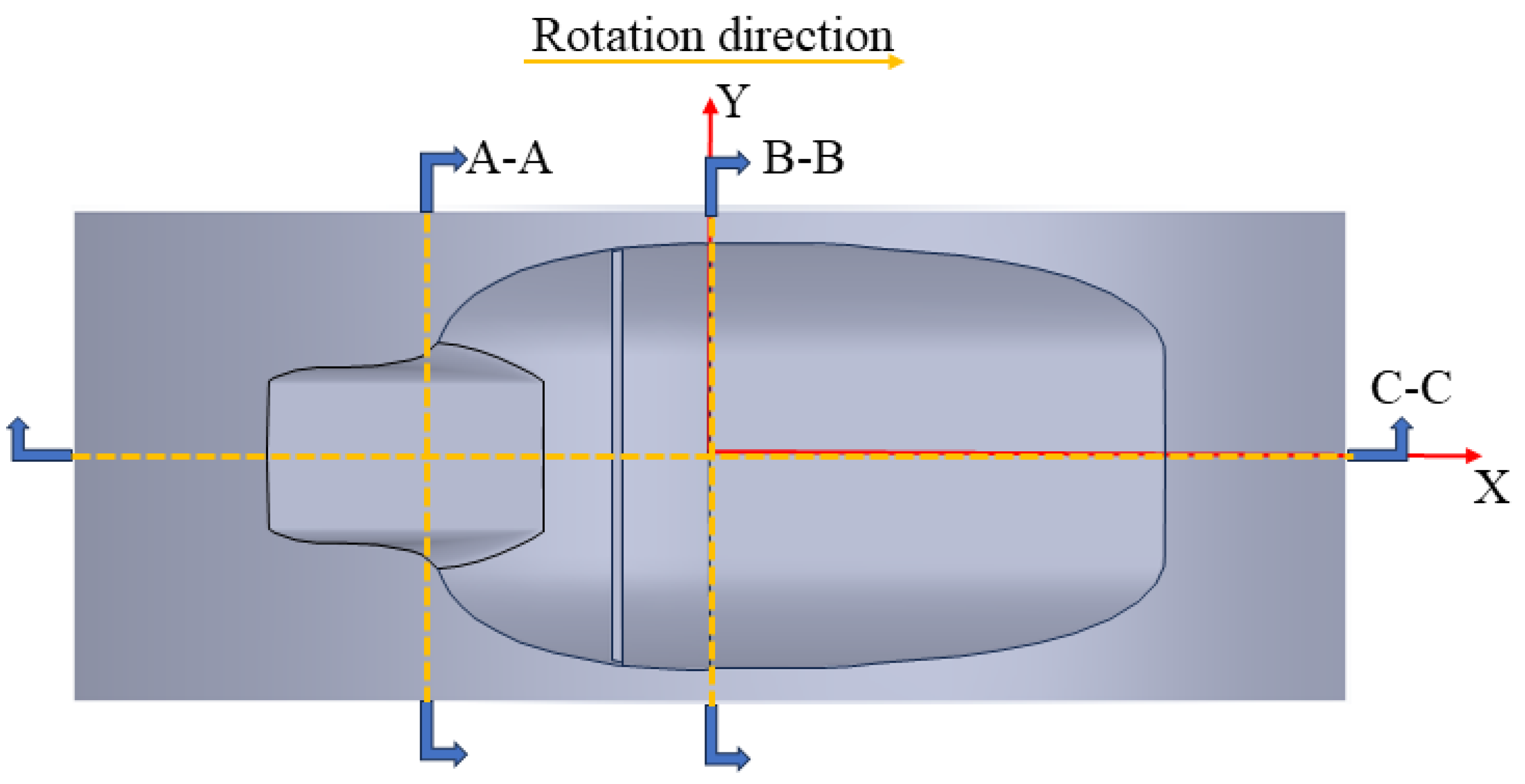
The rotor engine combustion is categorized into four parts: leading, middle, trailing, and spoiler. Rounded corners smooth the bottom surfaces. The cross sections of the leading, middle, and trailing parts of the combustion chamber are ovals formed by two semicircles and a rectangle, while the spoiler plate is a cuboid with a height below the rotor profile (Figure 1).

The Wankel engine’s combustion chamber consists of three elliptical cross sections and an oblong spoiler plate. The middle and trailing parts share the same cross-sectional dimensions but differ in inclination angles. Figure 2 and Figure 3 depict the size schematics, and

Table 2. Variable comparison.

Variable	Structure Name
r	Combustion chamber leading arc radius
l	Length of the leading bottom edge of the combustion chamber
h	The distance from the bottom of the combustion chamber’s leading section to the rotor’s center of gravity at the x-z plane
θ3	The angle between the combustion chamber’s leading bottom edge and the y-z plane
R	Trailing arc radius in the combustion chamber
L	Trailing bottom edge length of the combustion chamber
H	The distance from the bottom of the trailing section of the combustion chamber to the rotor’s center of gravity at the x-z plane
θ1	The angle between the middle bottom edge of the combustion chamber and the y-z plane
θ2	The angle between the trailing bottom edge of the combustion chamber and the y-z plane
a	The vertical distance between the spoiler plate and the rotor x-z section
b	The distance from the spoiler’s top center to the combustion chamber’s bottom edge
c	The spoiler plate’s width
q1	The excessive arc radius from the leading part to the middle of the combustion chamber
q2	The excessive arc radius from the middle to the trailing part of the combustion chamber

compares the variables and structural parameters.

To maintain the same compression ratio, the rotor combustion chamber must meet eight structural, process, and performance requirements:

(1)

The distance from the deepest part of the rotor combustion chamber to its center of gravity on the x-z plane must not exceed $h_{\alpha }$, considering structural strength, heat dissipation structure arrangement, and spindle assembly.

(2)

The maximum width of the chamber must not exceed $l_{\alpha }$, addressing seal arrangement and structural strength.

(3)

The distance between the chamber ends and the rotor tip on the y-z plane must not exceed $k_{\alpha }$, addressing radial seal arrangement and structural strength.

(4)

The width of the rotor spoiler plate must not exceed $c_{\alpha }$, ensuring spoiler plate strength.

(5)

According to research, the spoiler plate height should be at least ${\displaystyle \frac{4b_{\alpha }}{5}}$ [26,27,28,29,30], where $b_{\alpha }$ signifies the vertical distance from the chamber bottom to the rotor profile at the spoiler plate position.

(6)

To simplify processing, the rotor spoiler should be positioned centrally or toward the rear of the combustion chamber, avoiding overlap between chamber sections.

(7)

The leading and middle parts of the combustion chamber must be connected, with a single recess on the rotor surface.

(8)

The arc radius of the transition section must not exceed $q_{\alpha }$.

To ensure that the generated structural parameter combination meets the above requirements, the entire combustion chamber structure is parameterized first, so that a series of formulas can be used to calculate whether a certain structural combination meets the requirements of compression ratio, size, processing, and strength. When generating structural combinations, the values of several structural parameters are randomly generated within the required range of size, processing, and strength. Based on this, the compression ratio is used as the optimization objective; the size, processing, and strength requirements are used as the range; and the remaining structural parameters are used as the solving parameters for optimization iteration using optimization algorithms.

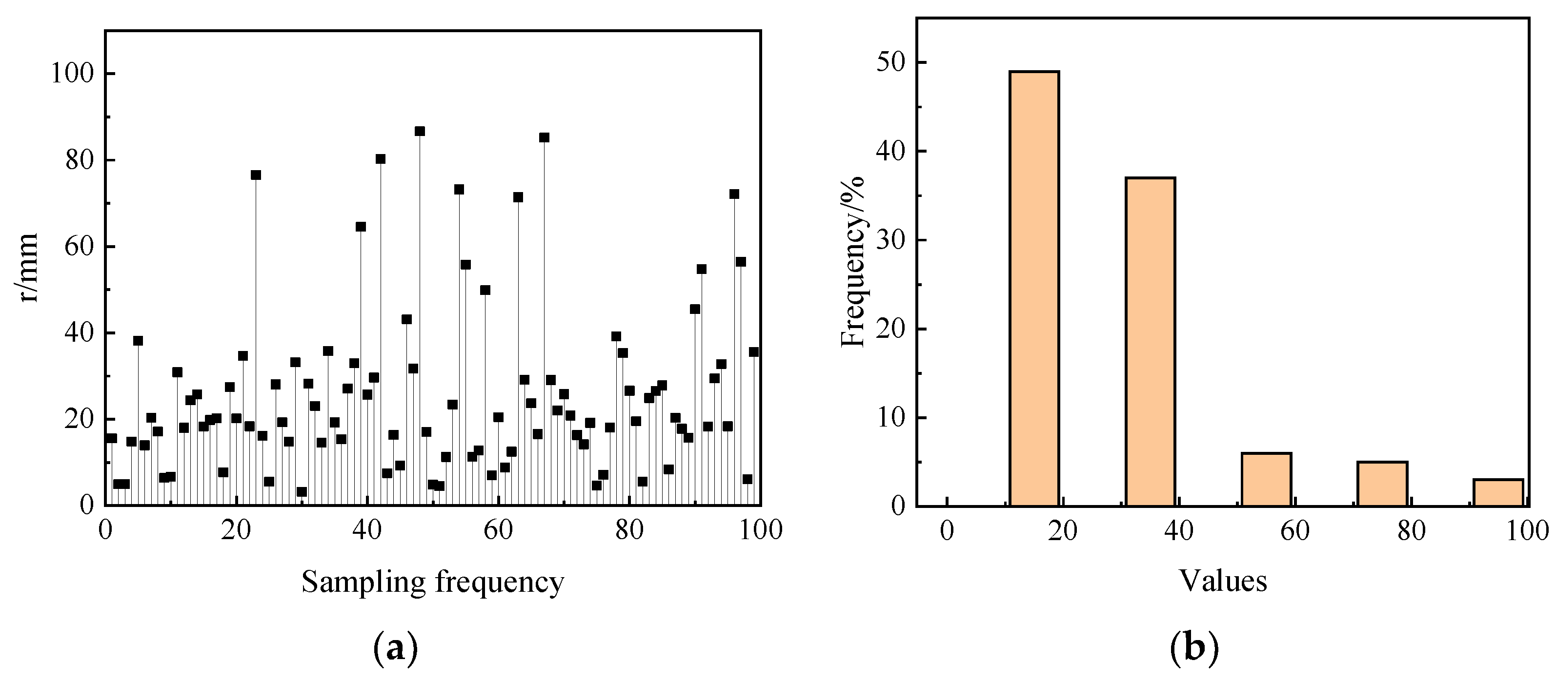
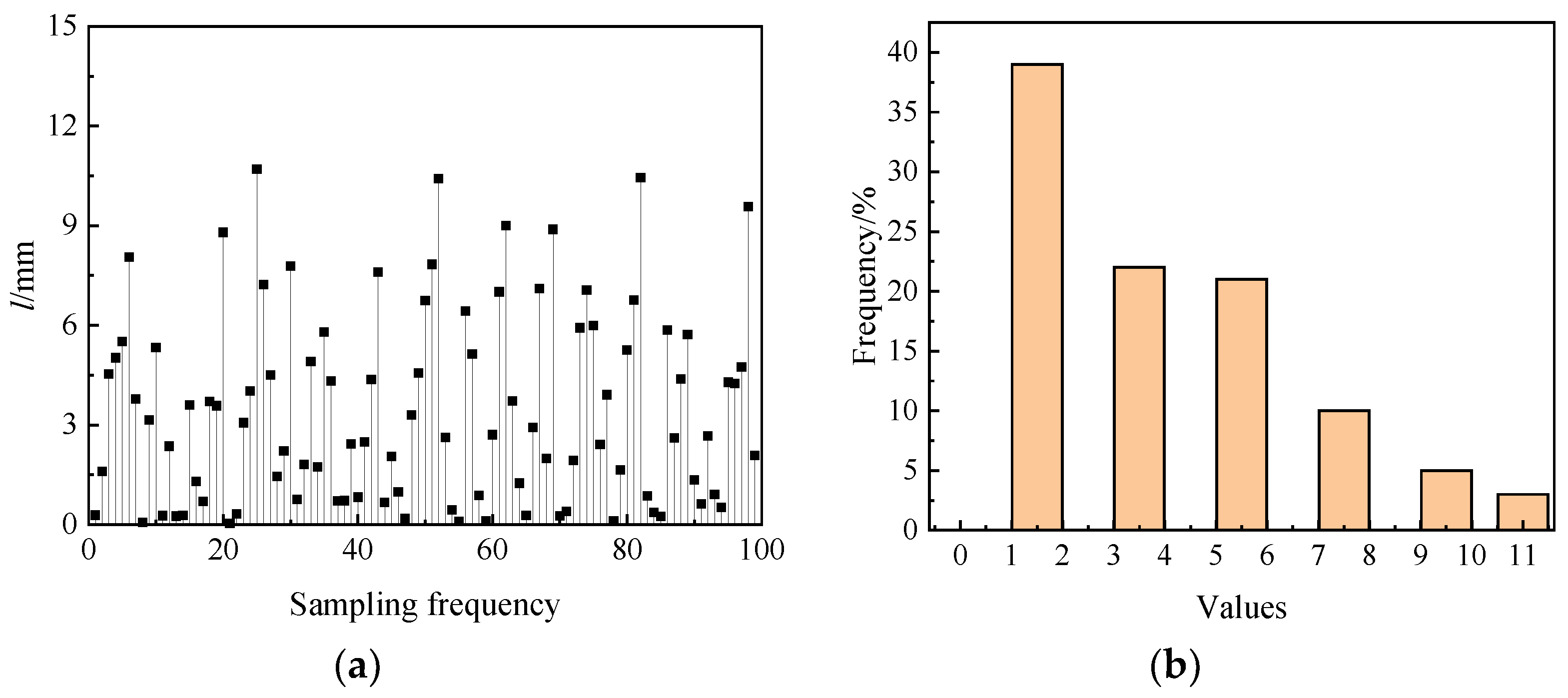
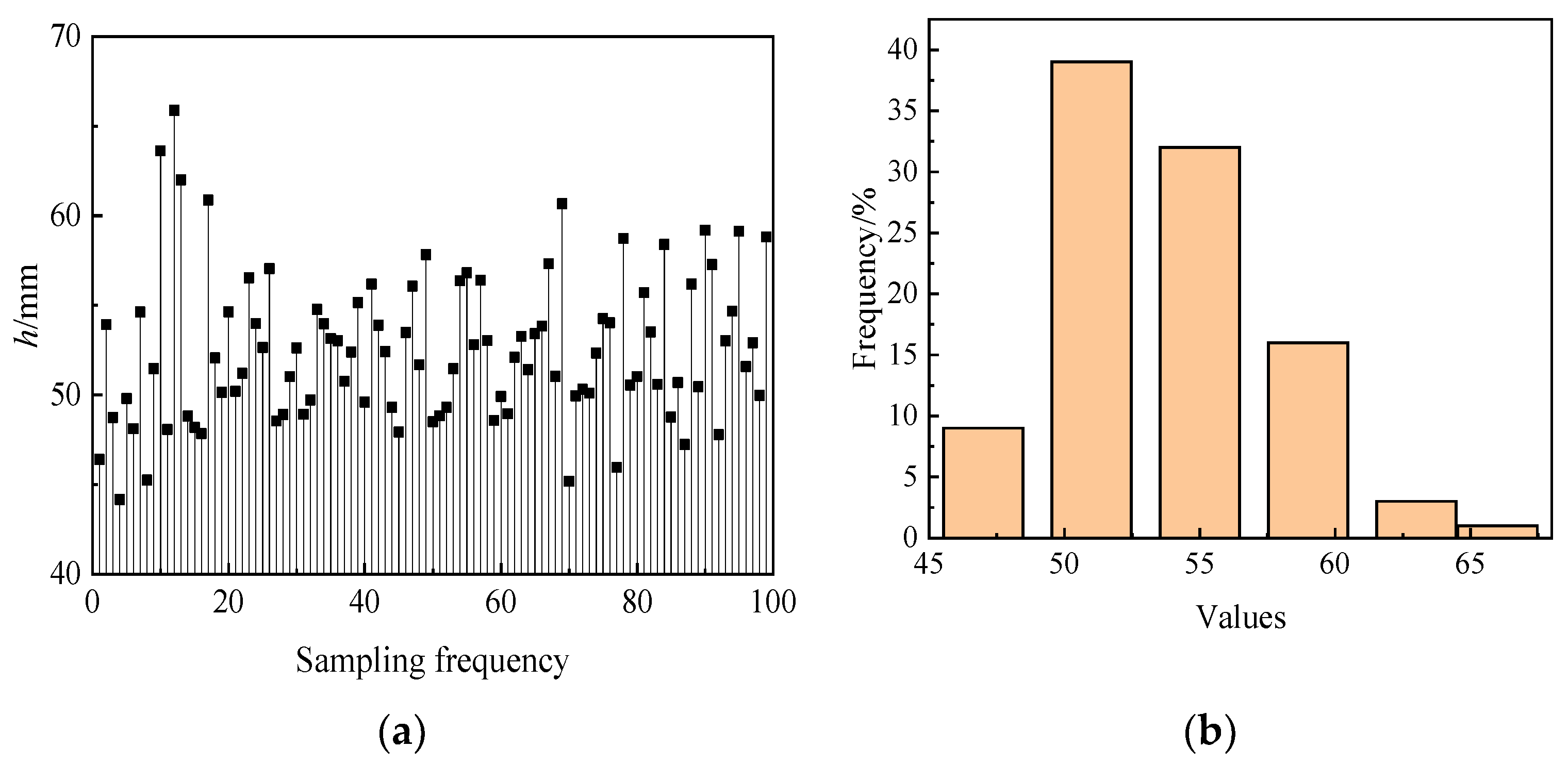
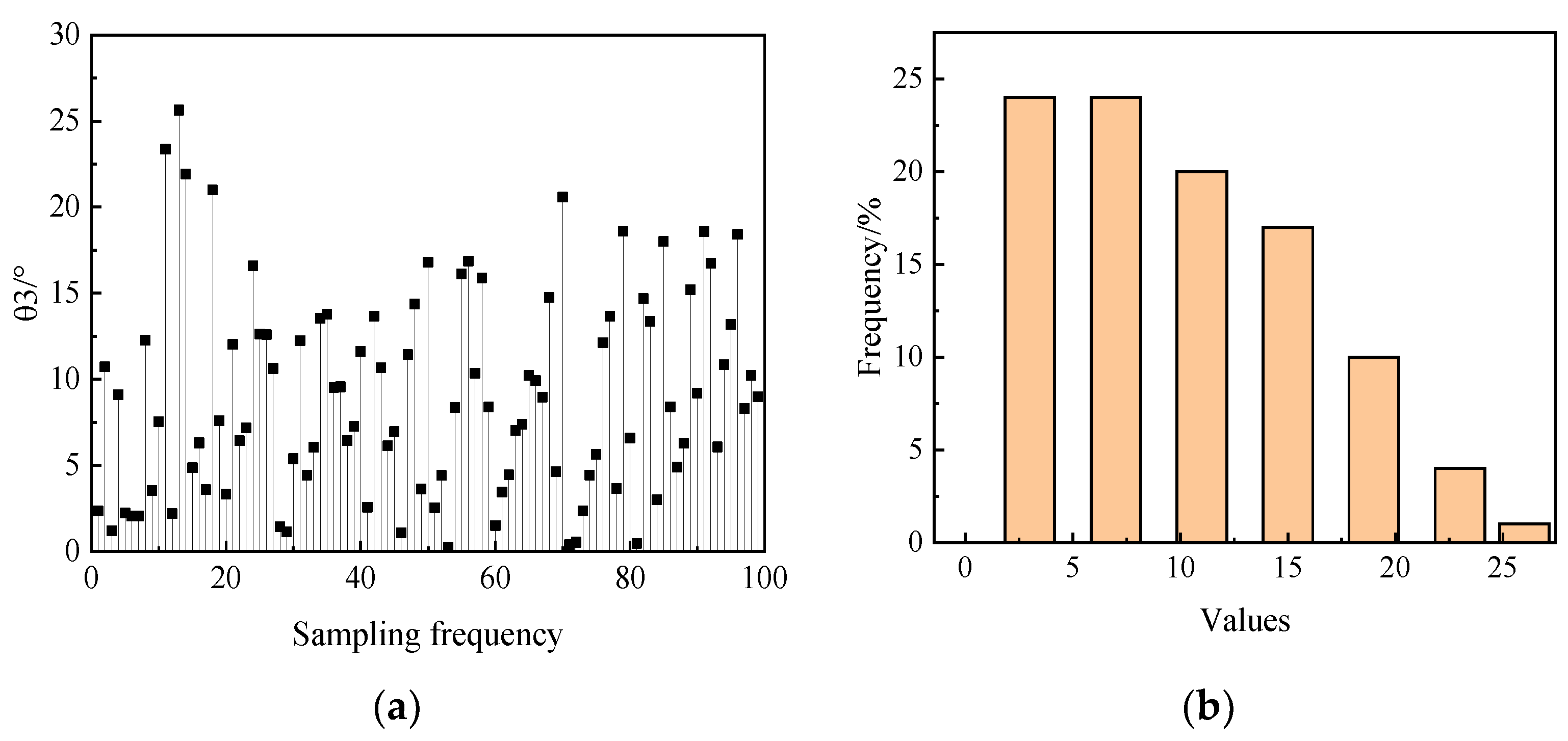
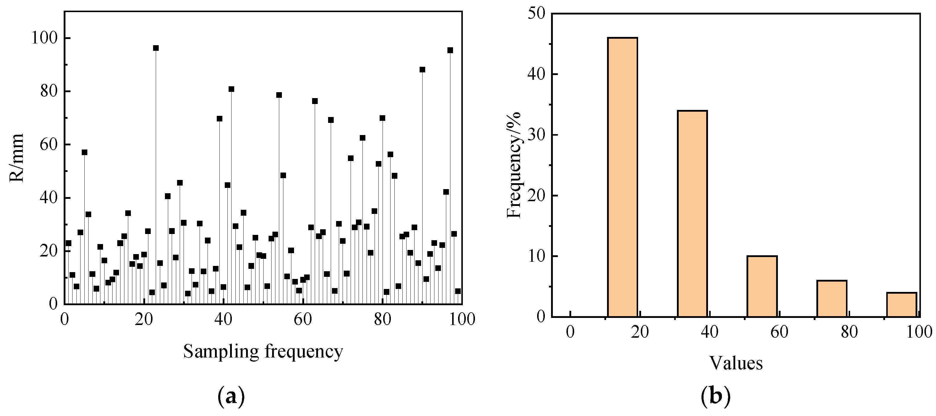
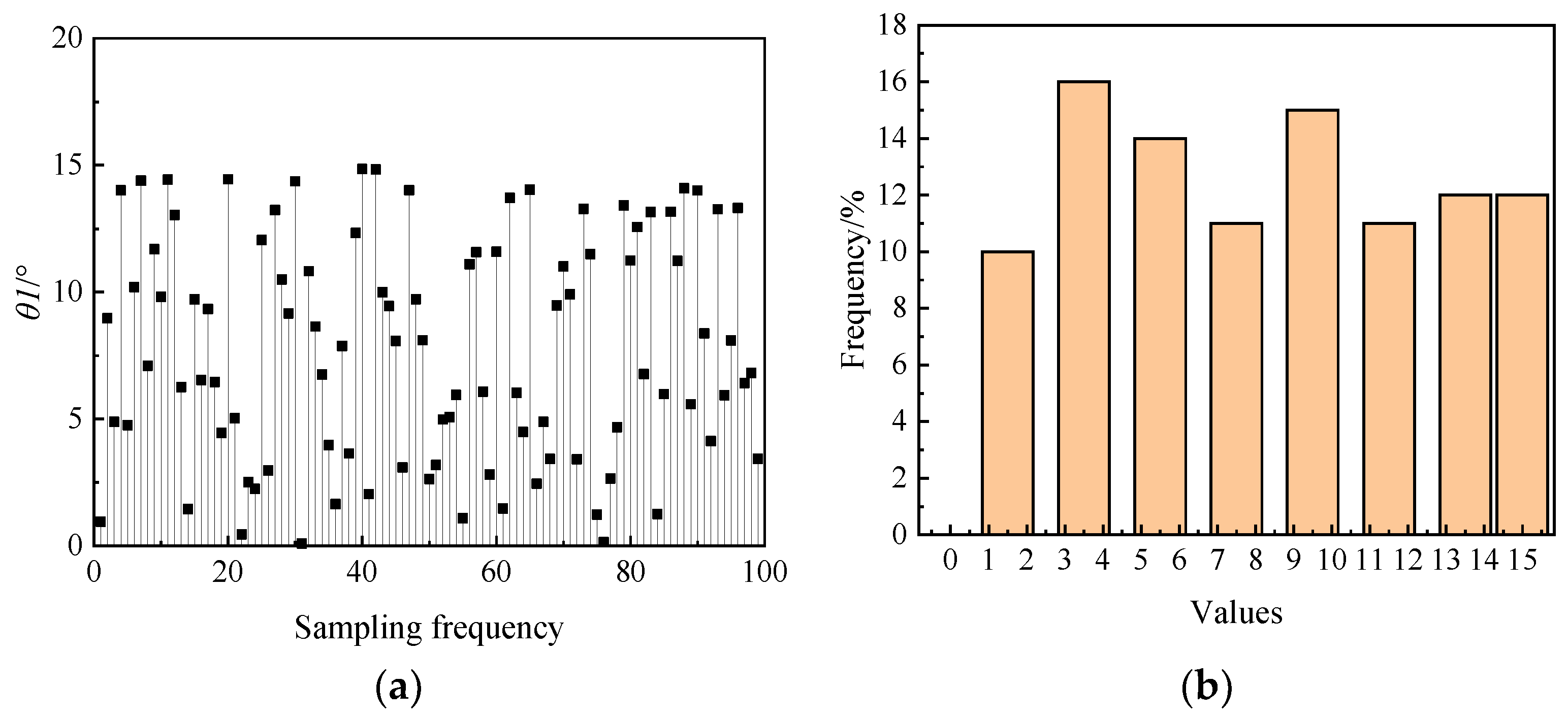
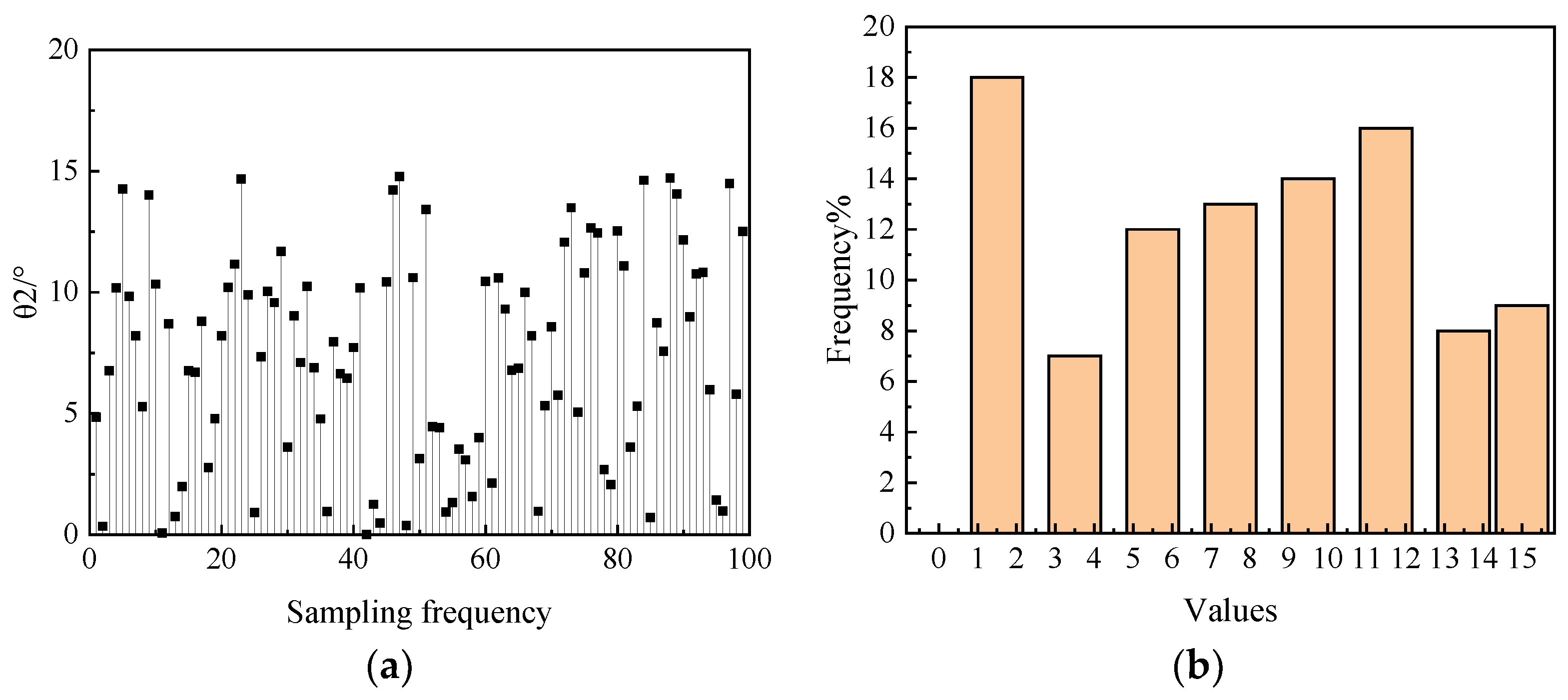
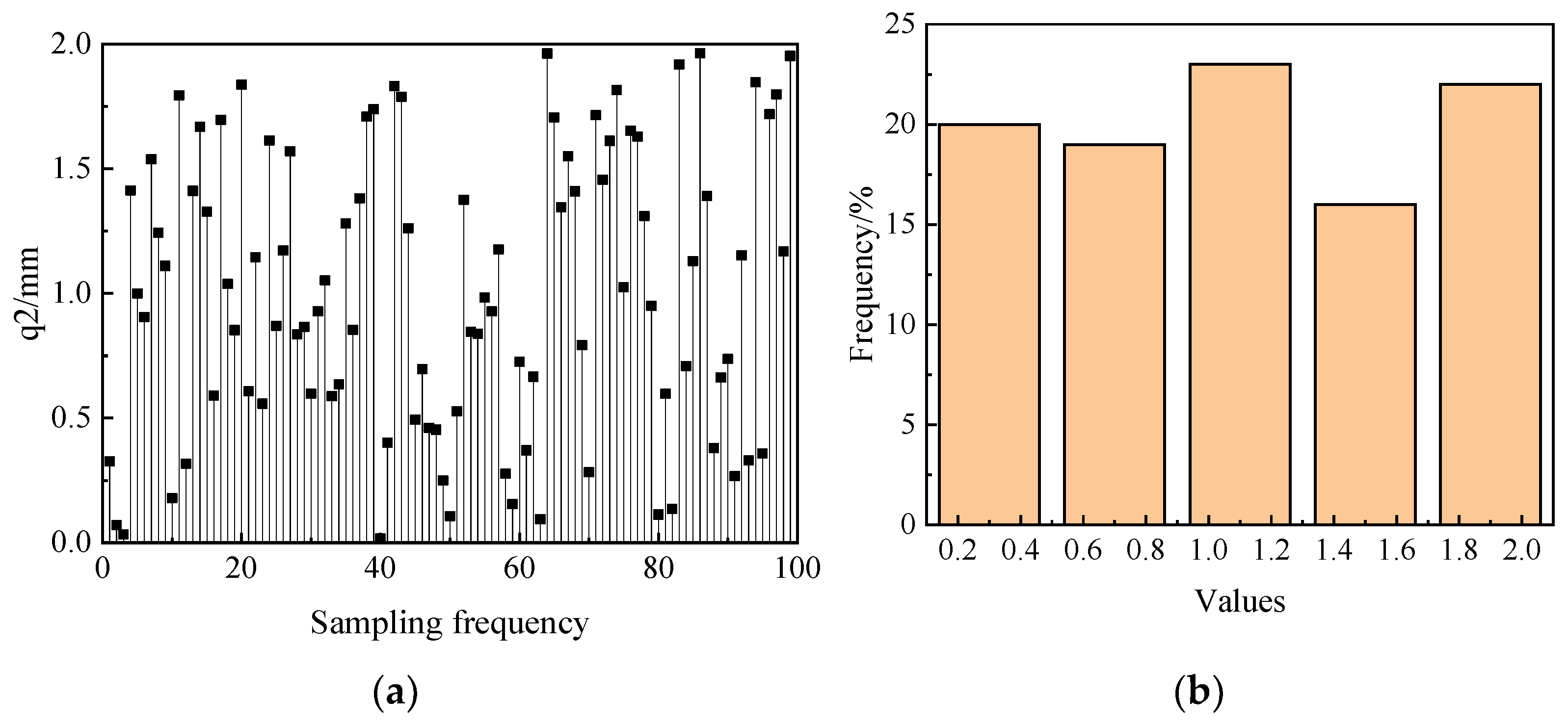
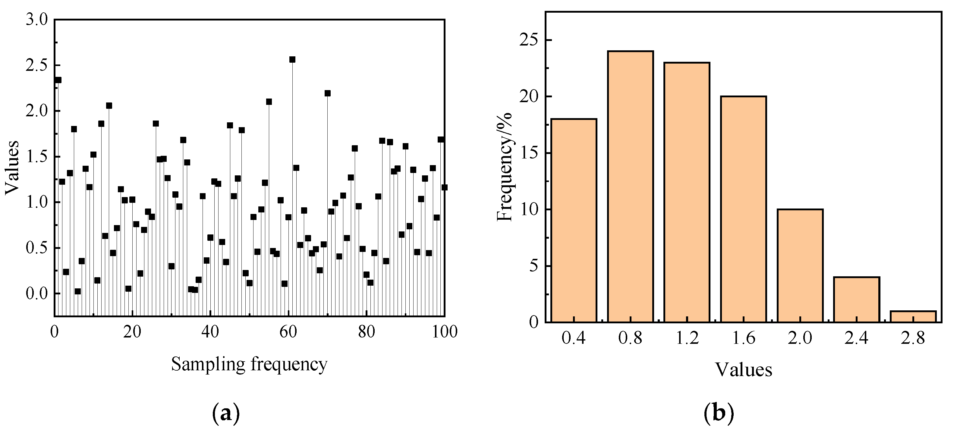
Using the parameters in

Table 3. Constraints.

Constraint Name	Variable Name	Value
The minimum distance from the bottom of the combustion chamber to the center of gravity of the rotor	$h_{\alpha }$	42 mm
Maximum width of the combustion chamber	$l_{\alpha }$	40 mm
The projection distance between the two ends of the rotor combustion chamber and the rotor tip on the y-z section	$k_{\alpha }$	10 mm
Maximum width of the spoiler plate	$c_{\alpha }$	3 mm
The maximum radius of the excessive arc	$q_{\alpha }$	2 mm

, 100 sets of structural parameter combinations were generated, including the 14 parameters listed. Figure 4, Figure 5, Figure 6, Figure 7, Figure 8, Figure 9, Figure 10, Figure 11, Figure 12, Figure 13, Figure 14, Figure 15, Figure 16 and Figure 17 depict their distribution and probabilities. From these figures, c, q1, and q2 follow a uniform distribution, while a follows a normal distribution. The distributions of r, l, h, θ3, R, L, H, θ1, θ2, and b are unclear, representing cognitive uncertainty. Consequently, the dimension reduction problem involves 14 dimensions with 4 random and 10 cognitive uncertainty variables.

3. Estimation Method of Active Subspace Eigenvalues Based on Probability Box–EDF

Recent advancements in dimensionality reduction techniques such as principal component analysis, factor analysis, topological mapping regression, and random projection have been significant [50,51,52]. Building on principal component analysis, the active subspace method evaluates input parameters through the output covariance matrix. This technique has been used in transonic wing design optimization, hydrological model construction, and satellite optimization, demonstrating benefits for complex system problems at high latitudes.

Unlike principal component analysis, which focuses on eigenvalue size impact on the covariance, the active subspace method constructs a new subspace by adjusting eigenvectors to significantly alter the system output direction [53,54]. For a system f with initial dimension n, its input x, output f, output function gradient f$\nabla$, and reduced dimension input v can be expressed as follows:

$$\left\{\begin{array}{c}x={\left[x_1,x_2,x_3,\dots ,x_n\right]}^T\\ f=f\left(x\right)\\ f\nabla =f\nabla \left(x\right)\\ v^{\prime }={\left[v_1^{\prime },v_2^{\prime },v_3^{\prime },\dots ,v_m^{\prime }\right]}^T\\ n>m\end{array}\right.$$

(1)

Normalizing each boundary of the standard parameter space to [0, 1] allows the non-standard parameter space to be transformed through regularization. The input parameter x with N samples can be expressed as follows:

$$X=\left\{x_{i,j};1\le i\le n,1\le j\le N\right\}$$

(2)

Any member of matrix X can be regularized as follows:

$$\left\{\begin{array}{c}{x}_{i,j}^{\prime }={\displaystyle \frac{x_{i,j}-\widehat{{\mu }_i}}{\widehat{{\sigma }_i}}}\\ \widehat{{\mu }_i}={\displaystyle \frac{1}{N}}{\displaystyle {\displaystyle \sum }_{j=1}^N}{x}_{i,j}\\ \widehat{{\sigma }_i}=\sqrt[2]{{\displaystyle \frac{1}{N}}{\displaystyle {\displaystyle \sum }_{j=1}^N}{\left(x_{i,j}-\overline{x_i}\right)}^2}\end{array}\right.$$

(3)

The gradient covariance matrix of f is as follows:

$$\left\{\begin{array}{c}C=\int f\nabla \left(\mathrm{x}\right)f\nabla {\left(\mathrm{x}\right)}^T\rho \left(x\right)dx=W\Lambda W^T\\ \Lambda =diag\left({\lambda }_1,{\lambda }_2,{\lambda }_3,\dots ,{\lambda }_n\right)\end{array}\right.$$

(4)

where W signifies an orthogonal matrix, Λ represents a non-negative eigenvalue matrix, and the eigenvalue’s relative size indicates the variables’ contribution to the objective function. In practical engineering, obtaining the transfer function $f\left(x\right)$ for the gradient covariance matrix is challenging, so the limited difference computation method is often used to calculate the sample outputs to derive $f\nabla$ and C [55,56]. The gradient covariance matrix can be expressed as follows:

$$C={\displaystyle \frac{1}{N}}{\displaystyle \sum }_{i=1}^{N}f{\nabla }_i\left(x\right)f{\nabla }_i{\left(x\right)}^T$$

(5)

The eigenvalues in matrix Λ are arranged in descending order, yielding ${\Lambda }^{\prime }=diag\left({\lambda }_1,{\lambda }_2,{\lambda }_3,\dots ,{\lambda }_n\right)$. The first m eigenvalues are chosen as the new active subspace dimensions, with the selection criteria shown in Equation (6).

$$\left\{\begin{array}{c}{\displaystyle \frac{{\lambda }_m}{{\sum }_{i=1}^n{\lambda }_i}}\ge k\\ {\displaystyle \frac{{\lambda }_{m+1}}{{\sum }_{i=1}^n{\lambda }_i}}\le k\end{array}\right.$$

(6)

where k denotes the proportional coefficient. The eigenvalue matrix ${\Lambda }^{\prime }$ is divided into the first m order ${\Lambda }_1^{\prime }$ and the last n-m order ${\Lambda }_2^{\prime }$.

$${\Lambda }^{\prime }=\left[\begin{array}{cc}{\Lambda }_1^{\prime }& \\ & {\Lambda }_2^{\prime }\end{array}\right]$$

(7)

Equation (4) can be expressed as

$$C=W\Lambda W^T=\left[U V\right]\left[\begin{array}{cc}{\Lambda }_1^{\prime }& \\ & {\Lambda }_2^{\prime }\end{array}\right]{\left[U V\right]}^T$$

(8)

where U denotes the basis vector for the active eigenvalue. After dimension reduction, the input v can be expressed as follows:

$$v=U^{T}x$$

(9)

The objective function can be approximated as follows:

$$f\left(x\right)\approx g\left(U^{T}x\right)$$

(10)

The error between the original and the dimension-reduced objective functions can be expressed as shown below:

$$\int f\left(x\right)-g\left(U^{T}x\right)\rho dx$$

(11)

The active subspace method, widely used across various fields, faces limitations due to input variable uncertainty. From Equation (4), the gradient covariance matrix of f can only be calculated if the probability distribution $\rho \left(x\right)$ of all input variables is known. Once this distribution is clear, the gradient covariance matrix can be calculated using the transfer function or samples, leading to the eigenvalue matrix Λ. Consequently, the subspace method for dimension reduction is applicable only if all input independent variables are random with a clear probability distribution. This limitation restricts the active subspace method’s use in engineering. Further research is needed on dimensionality reduction for cognitive and mixed uncertainty problems in engineering [57].

An objective function f with p random uncertainty variables, q cognitive uncertainty input independent variables, and n mixed uncertainty input independent variables can be expressed as follows:

$$\left\{\begin{array}{c}f=f\left(x_a,x_e\right)\\ x_a~\rho \left(x_a\right)\\ x_e\in \left[x_e^L,x_e^U\right]\\ x_a=\left\{x_{a1},x_{a2},x_{a3},\dots ,x_{ap}\right\}\\ x_e=\left\{x_{e1},x_{e2},x_{e3},\dots ,x_{eq}\right\}\end{array}\right.$$

(12)

The gradient of each independent variable can be expressed as

$${\nabla }_x{f}^I={\left[{\displaystyle \frac{\partial f}{\partial x_{a1}}}\dots {\displaystyle \frac{\partial f}{\partial x_{ap}}}{\displaystyle \frac{\partial f}{\partial x_{e1}}}\dots {\displaystyle \frac{\partial f}{\partial x_{eq}}}\right]}^T$$

(13)

where the real interval vector ${\nabla }_x{f}^I$, its upper limit $\overline{c_i}$, and its lower limit $\underset{¯}{c_i}$ can be expressed as follows:

$$\left\{\begin{array}{c}\overline{c_i}=max\left\{{\displaystyle \frac{\partial f}{\partial x_i}},x_a~\rho \left(x_a\right),x_e\in \left[x_e^L,x_e^U\right]\right\}\\ \underset{¯}{c_i}=min\left\{{\displaystyle \frac{\partial f}{\partial x_i}},x_a~\rho \left(x_a\right),x_e\in \left[x_e^L,x_e^U\right]\right\}\end{array}\right.$$

(14)

Combining Equations (13) and (14) indicates that when q = 0, ${\nabla }_x{f}^I={\nabla }_{x}f$. When q ≠ 0, the gradient covariance matrix C in Equation (4) can be expressed as

$$C={\widehat{C}}^I={\displaystyle \frac{1}{M}}{\displaystyle \sum }_{k=1}^M\left({\nabla }_x{f}_k^I\right)·{\left({\nabla }_x{f}_k^I\right)}^T$$

(15)

where ${\widehat{C}}^I$ is a real symmetric interval matrix with M samples. Each element in ${\widehat{C}}^I$ can be expressed as

$$\begin{gathered} {{\widehat{C}}^I}_{ij}={\displaystyle \frac{1}{M}}{\displaystyle \sum }_{k=1}^M\left({\displaystyle \frac{\partial f_k^I}{\partial x_i}}\right)·\left({\displaystyle \frac{\partial f_k^I}{\partial x_j}}\right) \\ =\left[{\underset{¯}{\widehat{C}}}_{ij},{\overline{\widehat{C}}}_{ij}\right] \\ =\left[{\displaystyle \frac{1}{M}}{\displaystyle \sum }_{k=1}^M{\underset{\_}{c}}_{ij}^k,{\displaystyle \frac{1}{M}}{\displaystyle \sum }_{i=1}^M{\overline{c}}_{ij}^k\right] \\ i,j=1,\dots ,n \end{gathered}$$

(16)

where $\left[{\underset{\_}{c}}_{ij}^k, {\overline{c}}_{ij}^k\right]$ can be expressed as follows:

$$\begin{gathered} \left[{\underset{\_}{c}}_{ij}^k, {\overline{c}}_{ij}^k\right]=\left[{\underset{\_}{c}}_i^k, {\overline{c}}_i^k\right]\times \left[{\underset{\_}{c}}_j^k, {\overline{c}}_j^k\right] \\ =\left[\min \left({\underset{\_}{c}}_i^k.{\underset{\_}{c}}_j^k,{\underset{\_}{c}}_i^k.{\overline{c}}_j^k,{\overline{c}}_i^k.{\underset{\_}{c}}_j^k,{\overline{c}}_i^k.{\overline{c}}_j^k\right),\max \left({\underset{\_}{c}}_i^k.{\underset{\_}{c}}_j^k,{\underset{\_}{c}}_i^k.{\overline{c}}_j^k,{\overline{c}}_i^k.{\underset{\_}{c}}_j^k,{\overline{c}}_i^k.{\overline{c}}_j^k\right)\right] \end{gathered}$$

(17)

Each feature pair in ${\widehat{C}}^I$ can be expressed as shown below:

$$\begin{gathered} \left({\lambda }_i^I,w_i^I\right) \\ i=1,\dots ,n \end{gathered}$$

(18)

Based on the analysis, the mixed uncertainty dimension reduction problem is transformed into the eigenvalue interval problem of ${\widehat{C}}^I$ expressed as follows:

$$\begin{gathered} {\lambda }^I=\left[\underset{\_}{\lambda },\overline{\lambda }\right] \\ =\left[{\underset{\_}{\lambda }}_i,{\overline{\lambda }}_i\right] \\ i=1,\dots ,n \end{gathered}$$

(19)

According to the Deif theorem, if a matrix retains the eigenvector component’s sign within the interval, the upper and lower bounds of the eigenvalues can be determined. The sign matrix that remains unchanged on ${\widehat{C}}^I$ is expressed as follows [58].

$$\begin{array}{r}{S}^i=diag\left(sgn\left(w_i\right)\right)\\ i=1,\dots ,n\end{array}$$

(20)

$$\left\{\begin{array}{c}\left({\widehat{C}}^c-S^i\Delta \widehat{C}{S}^i\right){\underset{\_}{w}}_i={\underset{\_}{\lambda }}_i{\underset{\_}{w}}_i\\ \left({\widehat{C}}^c+S^i\mathsf{\Delta }\widehat{C}{S}^i\right){\overline{w}}_i={\overline{\lambda }}_i{\overline{w}}_i\\ i=1,\dots ,n\end{array}\right.$$

(21)

where ${\widehat{C}}^c$ signifies the median matrix of ${\widehat{C}}^I$, and $\mathsf{\Delta }\widehat{C}$ represents the radius matrix of ${\widehat{C}}^I$, expressed as

$$\left\{\begin{array}{c}{\widehat{C}}^c=\left({\widehat{C}}_{ij}^c\right)={\displaystyle \frac{\widehat{\overline{C}}+\widehat{\underset{\_}{C}}}{2}}\\ {\widehat{C}}_{ij}^c={\displaystyle \frac{{\widehat{\overline{C}}}_{ij}+{\widehat{\underset{\_}{C}}}_{ij}}{2}}\\ i=1,\dots ,n\\ \Delta \widehat{C}=\left(\mathsf{\Delta }{\widehat{C}}_{ij}^c\right)={\displaystyle \frac{\widehat{\overline{C}}-\widehat{\underset{\_}{C}}}{2}}\\ \Delta {\widehat{C}}_{ij}^c={\displaystyle \frac{{\widehat{\overline{C}}}_{ij}-{\widehat{\underset{\_}{C}}}_{ij}}{2}}\\ i=1,\dots ,n\end{array}\right.$$

(22)

where $sgn\left(w_i\right)$ denotes the vector of the symbol function for each element of $w_i$. If all elements in $w_i$ have the same sign, then the following is true:

$$\left\{\begin{array}{c}\widehat{\underset{\_}{C}} {\underset{\_}{w}}_i={\underset{\_}{\lambda }}_i{\underset{\_}{w}}_i\\ \overline{\widehat{C}} {\overline{w}}_i={\overline{\lambda }}_i{\overline{w}}_i\\ i=1,\dots ,n\end{array}\right.$$

(23)

The maximum and minimum values of $\left|w_i\right|$ can be computed as follows, where I is the unit matrix.

$$\left\{\begin{array}{c}{\lambda }_i-\Delta \widehat{C}\left|w_i\right|\le \left({\lambda }_{i}I-S^i{\widehat{C}}^c{S}^i\right)\left|w_i\right|\le \Delta \widehat{C}\left|w_i\right|\\ \left[\begin{array}{c}{\lambda }_{i}I-S^i{\widehat{C}}^c{S}^i-\Delta \widehat{C}\\ {\widehat{C}}^c{S}^i-{\lambda }_{i}I-\Delta \widehat{C}\end{array}\right]\left|w_i\right|\le 0\\ i=1,\dots ,n\end{array}\right.$$

(24)

A positive semi-definite real symmetric matrix C has an orthogonal matrix W, such that

$$W^T\widehat{C}W=diag\left({\lambda }_1,{\lambda }_2,\dots ,{\lambda }_n\right)$$

(25)

For $\wedge =diag\left({\lambda }_1,{\lambda }_2,\dots ,{\lambda }_n\right)$, we have

$$\left\{\begin{array}{c}{\left(W{w}_i\right)}^T\widehat{C}W{w}_i=w_i^T\wedge w_i={\lambda }_1{w}_1^2+{\lambda }_2{w}_2^2+\dots +{\lambda }_n{w}_n^2\ge 0\\ w_i={\left[w_1,w_2,\dots ,w_n\right]}^T\\ {\lambda }_i\ge 0\\ i=1,\dots ,n\end{array}\right.$$

(26)

where

$$\begin{gathered} {\lambda }_i=w_i^T\widehat{C}{w}_i \\ \begin{array}{l}=w_i^T\left[{\displaystyle \frac{1}{M}}{\displaystyle \sum _{k=1}^M}\left({\nabla }_x{f}_k^I\right)·{\left({\nabla }_x{f}_k^I\right)}^T\right]w_i\\ ={\displaystyle \frac{1}{M}}{\displaystyle \sum _{k=1}^M}{\left[{\left({\nabla }_x{f}_k\right)}^T{w}_i\right]}^2\ge 0\end{array} \\ i=1,\dots ,n \end{gathered}$$

(27)

where $w_i$ denotes the effect of the i-th input variable on the objective function. Combined with Equations (4)–(11), it yields dimensionality reduction of mixed uncertainty.

In deriving a mixed uncertainty dimension reduction problem from Equations (20)–(27), a key requirement is that the gradient covariance matrix ${\widehat{C}}^I$ must satisfy the Deif theorem, maintaining the sign of eigenvector components within the interval. In practice, it is challenging to verify without the objective function (f) or sufficient data. To tackle large computational load, dimensionality, and prior condition challenges in mixed uncertainty reduction, eigenvalue estimation techniques and gradient response estimation approaches have been proposed. The former include the disc method, perturbation method, and spectral radius method. The latter represent direct optimization, eigenvalue analysis, and modal decomposition. Eigenvalue methods only approximate ranges and cannot obtain upper and lower bounds, while gradient response methods lose accuracy with high system uncertainty [50].

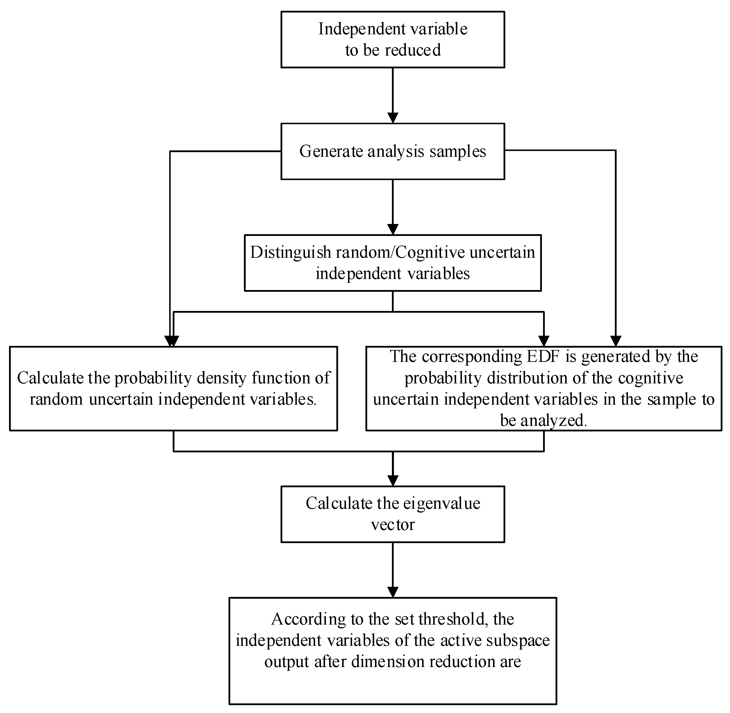
This study proposes a mixed uncertainty eigenvalue estimation method using the EDF and probability boxes [59,60,61] for dimension reduction, as illustrated in Figure 18.

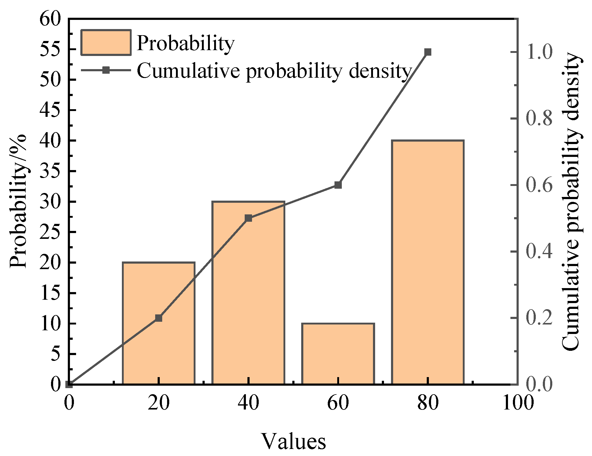
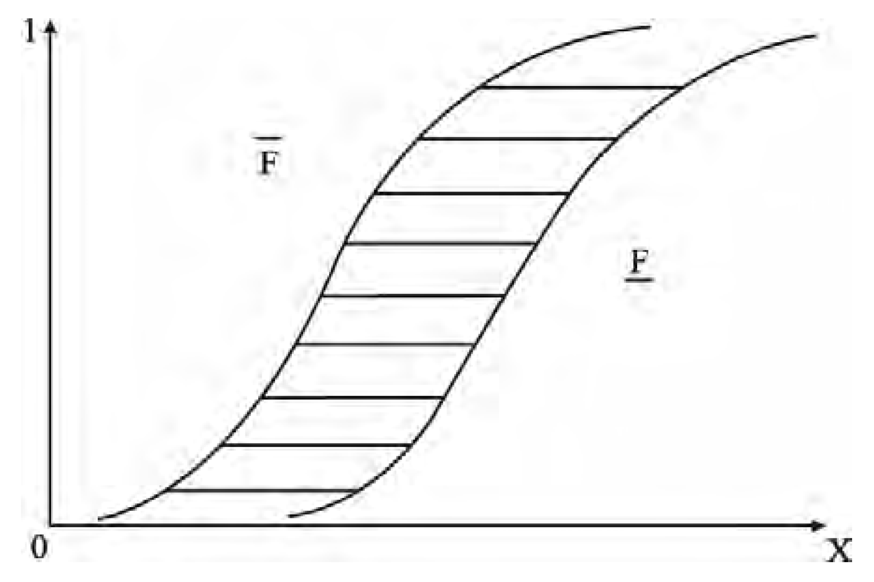
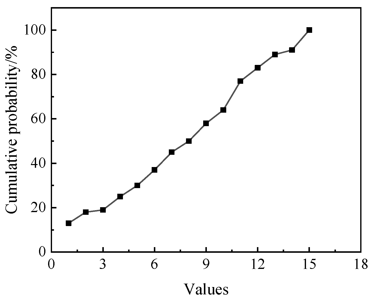
The EDF describes variable distributions by approximating sample frequencies to the probability distribution of random variables as a step function, resulting in the Cumulative Distribution Function (CDF). This method converts the mixed uncertainty dimension reduction into a random uncertainty problem. Figure 19 shows a CDF with an EDF distribution, where the black line shows the EDF fit and the histogram indicates variable probabilities [62,63].

In practice, due to randomness in input variables, the empirical density is fitted using an equal distribution model. The empirical density function for mixed uncertainty is

$${\widehat{F}}_n\left(x\right)={\displaystyle \frac{{\sum }_{i=1}^{n}I\left(X_i\le x_i\right)}{n}}$$

(28)

where the EDF is fitted by ${\widehat{F}}_n\left(x\right)$; $X_i$ represents an independent and identically distributed random variable; $x_i$ denotes the function value of the empirical distribution function at x; and n signifies the number of samples. The accuracy of the empirical density function increases with more samples.

All cognitive uncertainty variables can be expressed as random uncertainty variables.

$$\begin{gathered} y={\widehat{W}}_1^T\left(x_a,x_e\right) \\ {x}_a~{\rho }_{x_a},x_e~{\rho }_{x_e} \end{gathered}$$

(29)

where ρ _ (x _ a) and ρ _ (x _ e) denote the sampling weights of random and cognitive uncertainties based on the distribution function and fitted differential EDF, respectively. Integrating these variables into the equation yields the following:

$$C={\displaystyle \frac{1}{N}}{\displaystyle \sum }_{i=1}^N\mathrm{y}{\nabla }_i\left(x\right)y{\nabla }_i{\left(x\right)}^T$$

(30)

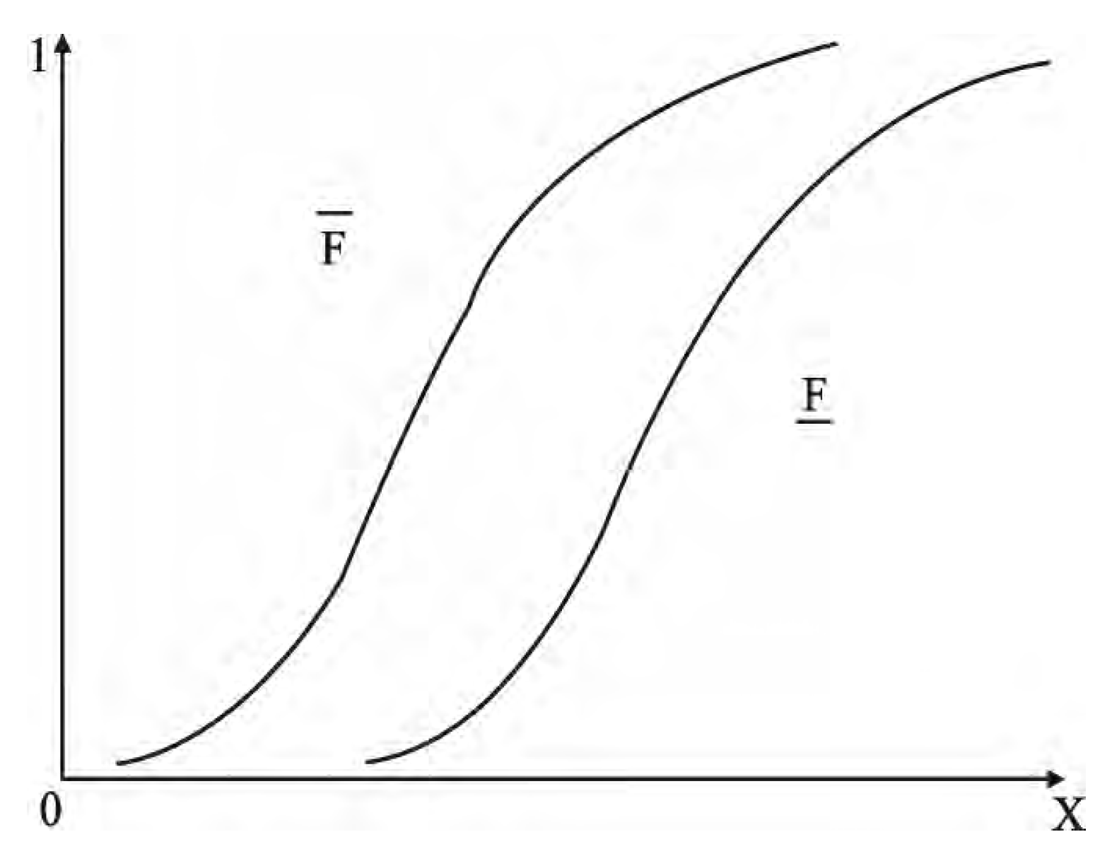
Eigenvalues for the mixed uncertainty active subspace are determined using Equation (27), enabling mixed uncertainty dimensionality reduction. Probability boxes representing variable distributions are used to obtain EDF curves. These boxes incorporate interval concepts for both random and cognitive uncertainties. Figure 20 illustrates a probability box variable x with cumulative distribution function ${\widehat{F}}_n\left(x\right)$, upper bound $\overline{{\widehat{F}}_n}\left(x\right)$, and lower bound $\underset{¯}{{\widehat{F}}_n}\left(x\right)$. The probability box requires only upper and lower distribution bounds to split the boundary around the variable distribution function, eliminating the need for specific distribution forms and ensuring that the cumulative distribution function lies within the defined boundaries.

To obtain the probability box of variables, we use the D-S theory composed of multiple focal elements. For a sample in space R, any D-S structure can be expressed as

$$\left\{\begin{array}{c}m:2^R\to \left[0,1\right]\\ m\left(\varnothing \right)\ne 0,{{\displaystyle \sum }}_{A\subseteq R}m\left(A\right)=1\end{array}\right.$$

(31)

where each interval A is a focal element; $m\left(A\right)$ denotes the reliability value corresponding to this focal element; and $2^R$ signifies the power set of R. The trust function Bel and the likelihood function Pl can be expressed as follows:

$$\left\{\begin{array}{c}Bel\left(A\right)=\sum \left\{m\left(B\right)|B\subseteq A,B\ne \varnothing \right\}\\ Pl\left(A\right)=\sum \left\{m\left(B\right)|A\cap B,B\ne \varnothing \right\}\end{array}\right.$$

(32)

Probability boxes consist of multiple D-S structures, the upper and lower bounds of which are accumulated to attain the left boundary of the upper and lower bounds of the probability box. The D-S structure represents a discretized probability box. Figure 21 illustrates the relationship between the probability box and the structure. EDF fitting using probability boxes is conducted as follows:

Step 1:

Resample N samples into N groups, and divide each group into M segments from largest to smallest.

Step 2:

Use each segment’s maximum and minimum values as upper and lower bounds, respectively. If the distribution aligns with a certain distribution model, the upper and lower bounds of each group’s probability are obtained based on the distribution model; otherwise, the bounds are obtained based on the EDF probability distribution in Equation (28).

Step 3:

Average the maximum upper bounds and minimum lower bounds across N groups to obtain the fitted cumulative probability curve.

To verify the accuracy of the above methods, this study evaluates an objective function with random and cognitive uncertainties, as shown in Equation (33), where $x_1$ denotes a random variable uniformly distributed in [0, 1], and $x_2$ represents a cognitive variable in [0, 3]. Figure 22 shows the distribution and probabilities from 100 samples, which do not fit any standard distribution model.

$$f\left(x_1,x_2\right)=e^{x_1}+x_2+x_1{x}_2$$

(33)

Equation (4) shows that with M samples, the gradient covariance matrix C of $f\left(x_1,x_2\right)$ can be expressed as follows:

$$\begin{array}{c}C={\widehat{C}}^I={\displaystyle \frac{1}{M}}{\displaystyle {\displaystyle \sum }_{k=1}^M}\left({\nabla }_x{f}_k^I\right)·{\left({\nabla }_x{f}_k^I\right)}^T\\ ={\displaystyle \frac{1}{M}}{\displaystyle {\displaystyle \sum }_{k=1}^M} \left[\begin{array}{cc}\left[e^{2x_1},e^{2x_1}+6e^{x_1}+9\right]& \left[\left(x_1+1\right)e^{x_1},\left(x_1+1\right)e^{x_1}+3\left(x_1+1\right)e^{x_1}+3\right]\\ \left[\left(x_1+1\right)e^{x_1},\left(x_1+1\right)e^{x_1}+3\left(x_1+1\right)e^{x_1}+3\right]& x_1^2+2x_1+1\end{array}\right]\end{array}$$

(34)

The EDF obtained by probability box fitting is shown in Figure 23.

With M = 100 samples, eigenvalues ${\lambda }_1$, ${\lambda }_2$, and their proportions, obtained using computation Equations 33 and 34 probability box–EDF estimation, are shown in

Table 4. Eigenvalue calculation results.

Eigenvalue Calculation Method	${\mathit{\lambda }}_1$	${\mathit{\lambda }}_1$ Proportion	${\mathit{\lambda }}_2$	${\mathit{\lambda }}_2 \mathbf{Proportion}$
Formula calculation	12.3058	62.1078%	7.5078	37.8922%
Probability box–EDF estimation	12.8423	60.8148%	8.2748	39.1852%

. The proposed method achieves high accuracy, with a deviation of only 1.2931%, making it effective for eigenvalue calculation and dimensionality reduction in rotor engine combustion chambers.

4. Dimensionality Reduction Analysis of Combustion Chamber Structure Parameters

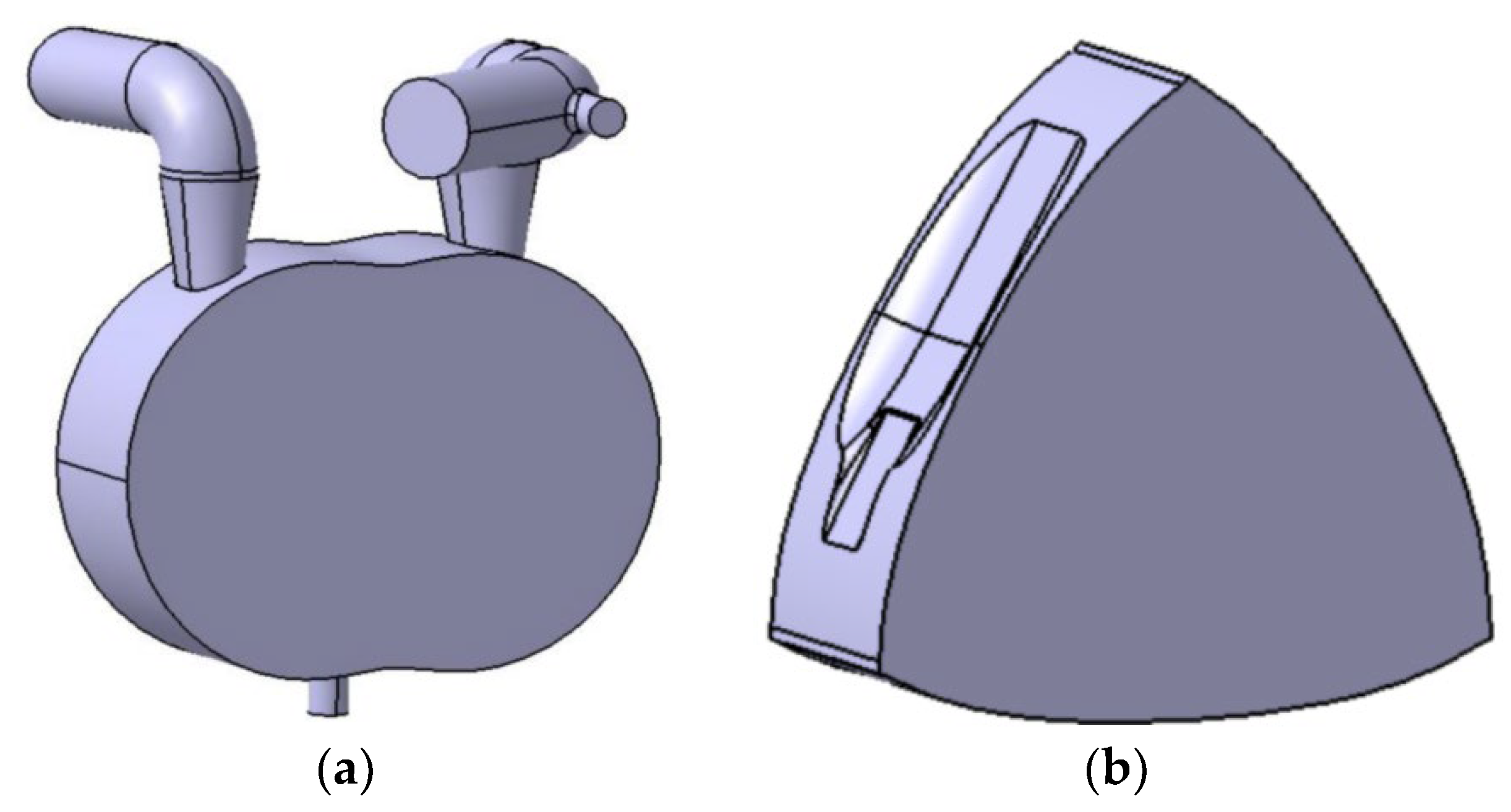
This paper uses peak cylinder pressure and temperature as performance indicators. With

Table 5. Rotor engine boundary conditions.

Boundary	Type	Temperature (K)	Pressure (MPa)
Inlet	Inflow	300	0.101325
Intake port	Fixed wall	300	/
Outlet	Outflow	570	0.101325
Exhaust port	Fixed wall	550	/
Rotor	Moving wall	400	/
Rotor flank 1	Fixed wall	624	0.117210
Rotor flank 2	Fixed wall	600	/

showing the boundary conditions, the RNG K-ε model calculates cylinder airflow [64,65,66]. The PRF skeleton mechanism with 41 components and 124 chemical reactions is combined with the SAGE chemical kinetic model for combustion calculations [67,68]. Figure 24 depicts solid model parameters [58].

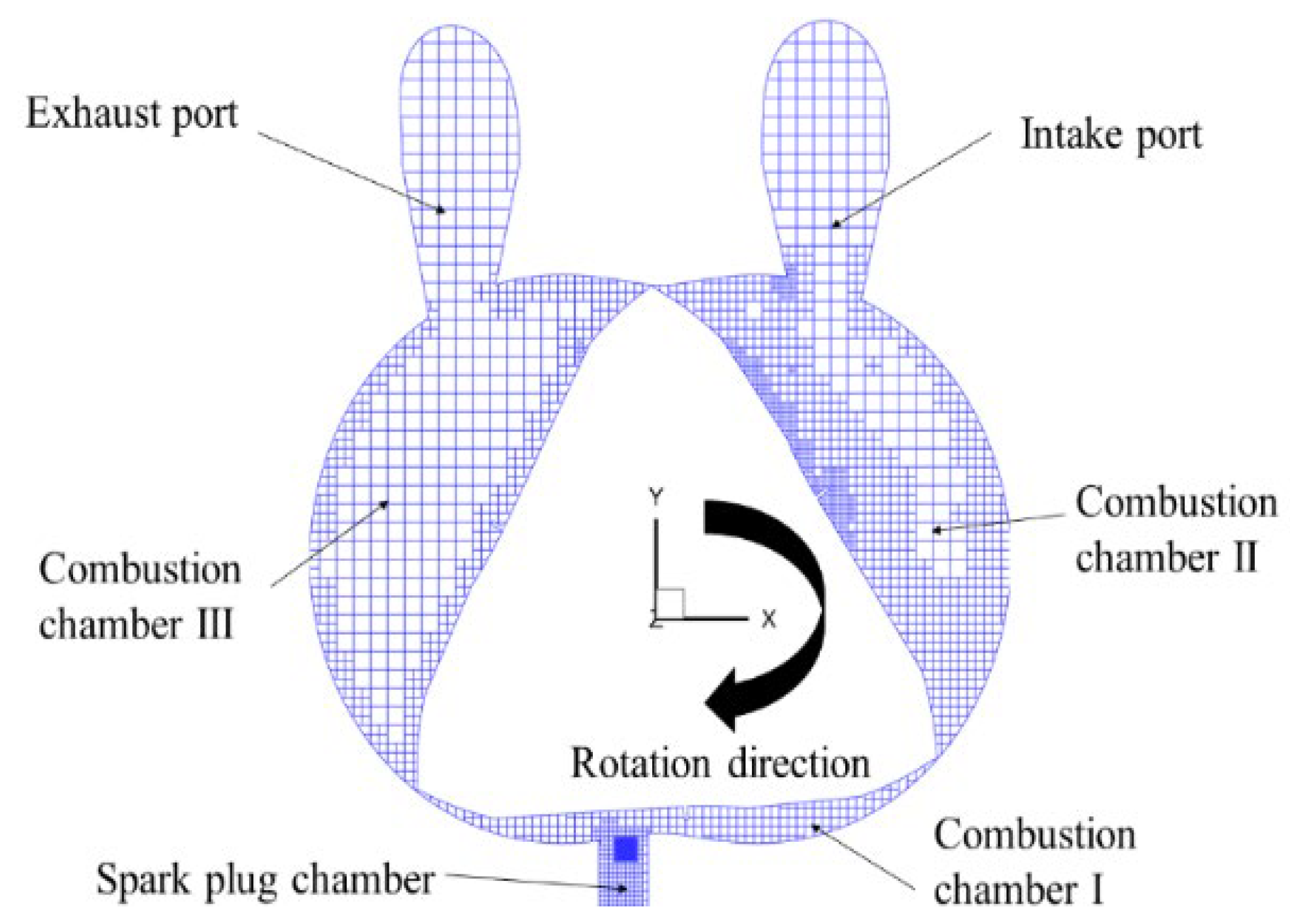
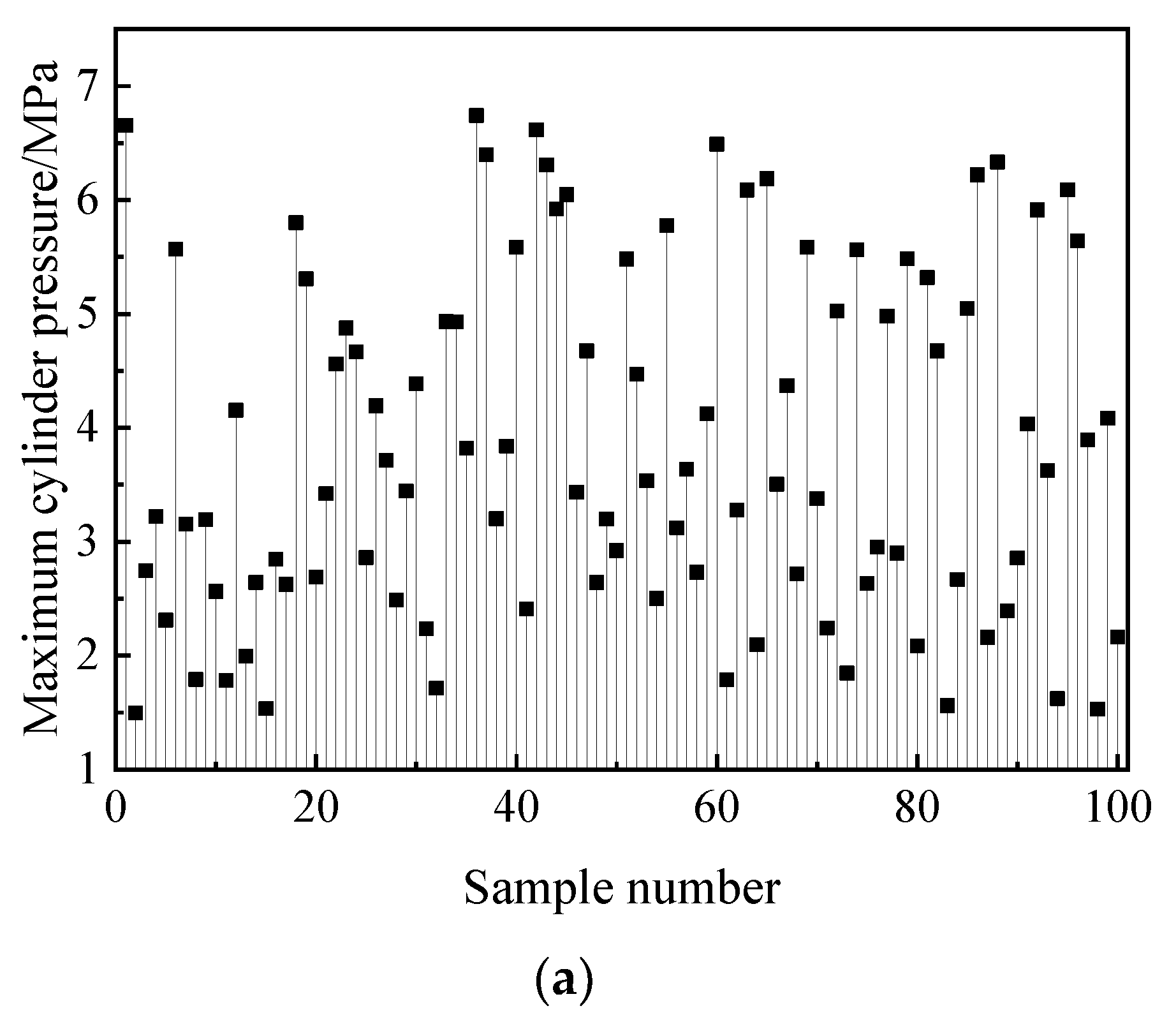
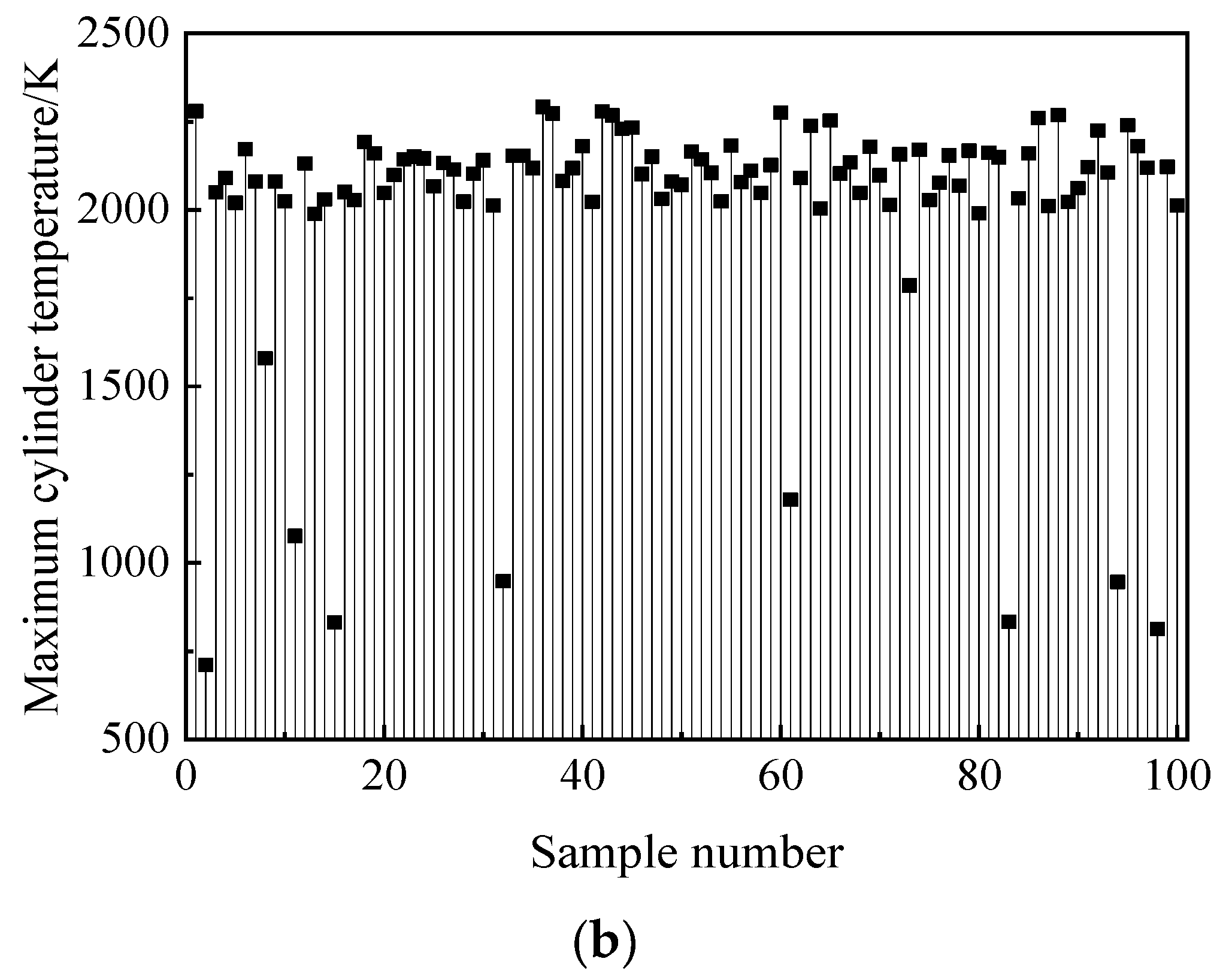
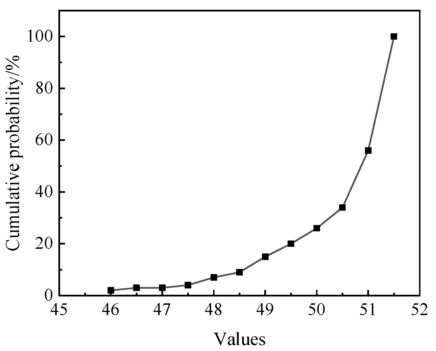
Grid number affects calculation results. To eliminate this influence, ensure accuracy, and select the optimal grid number to reduce computation time, grid independence analysis of the simulation model is necessary. This study compares in-cylinder pressure changes under four different grid sizes with constant boundary conditions set as shown in Table 5. Figure 25 shows pressure change curves for different grid sizes. Adaptive mesh refinement (AMR) [69,70,71] is applied to a 2 mm mesh, producing results consistent with a 1 mm mesh size and achieving stable calculations. Considering efficiency, accuracy, and calculation time, a 2 mm mesh is selected, resulting in approximately 200,000 hexahedral element grids, as shown in Figure 26. The 100 parameter combinations obtained in Section 2 are calculated with performance indices (Figure 27).

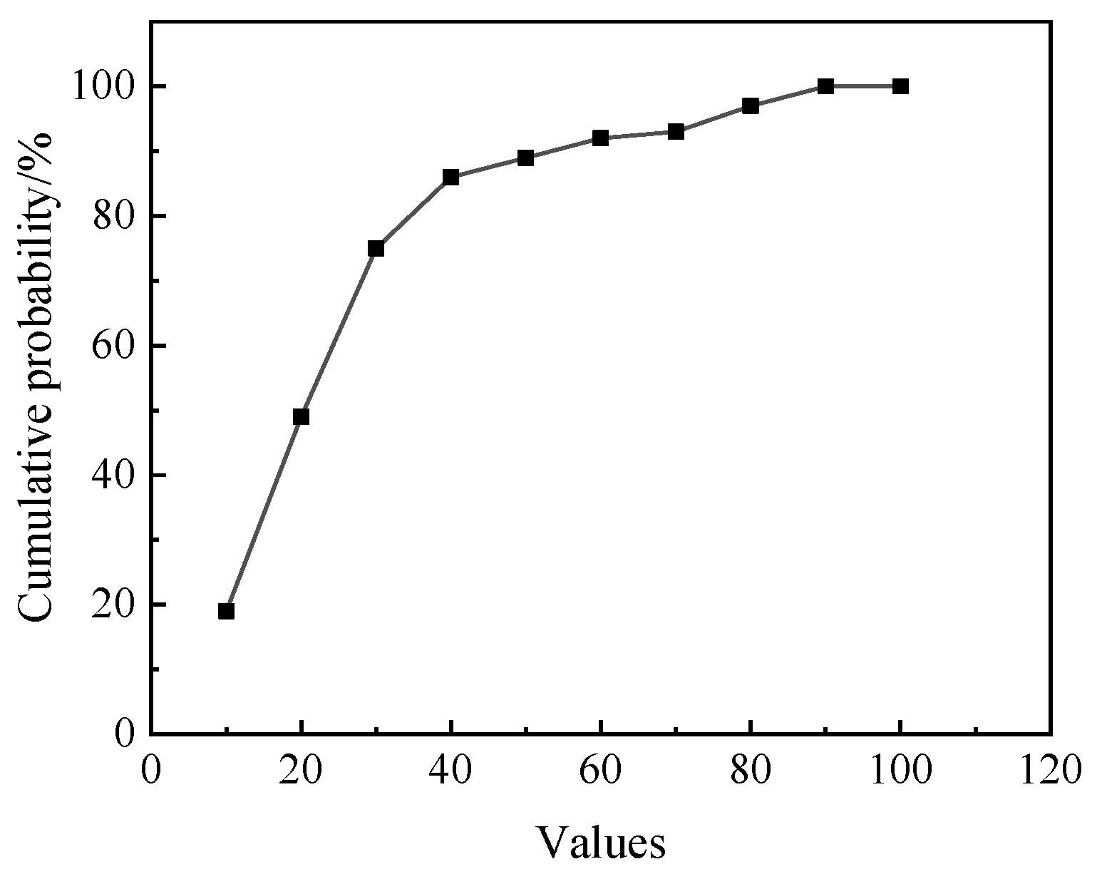
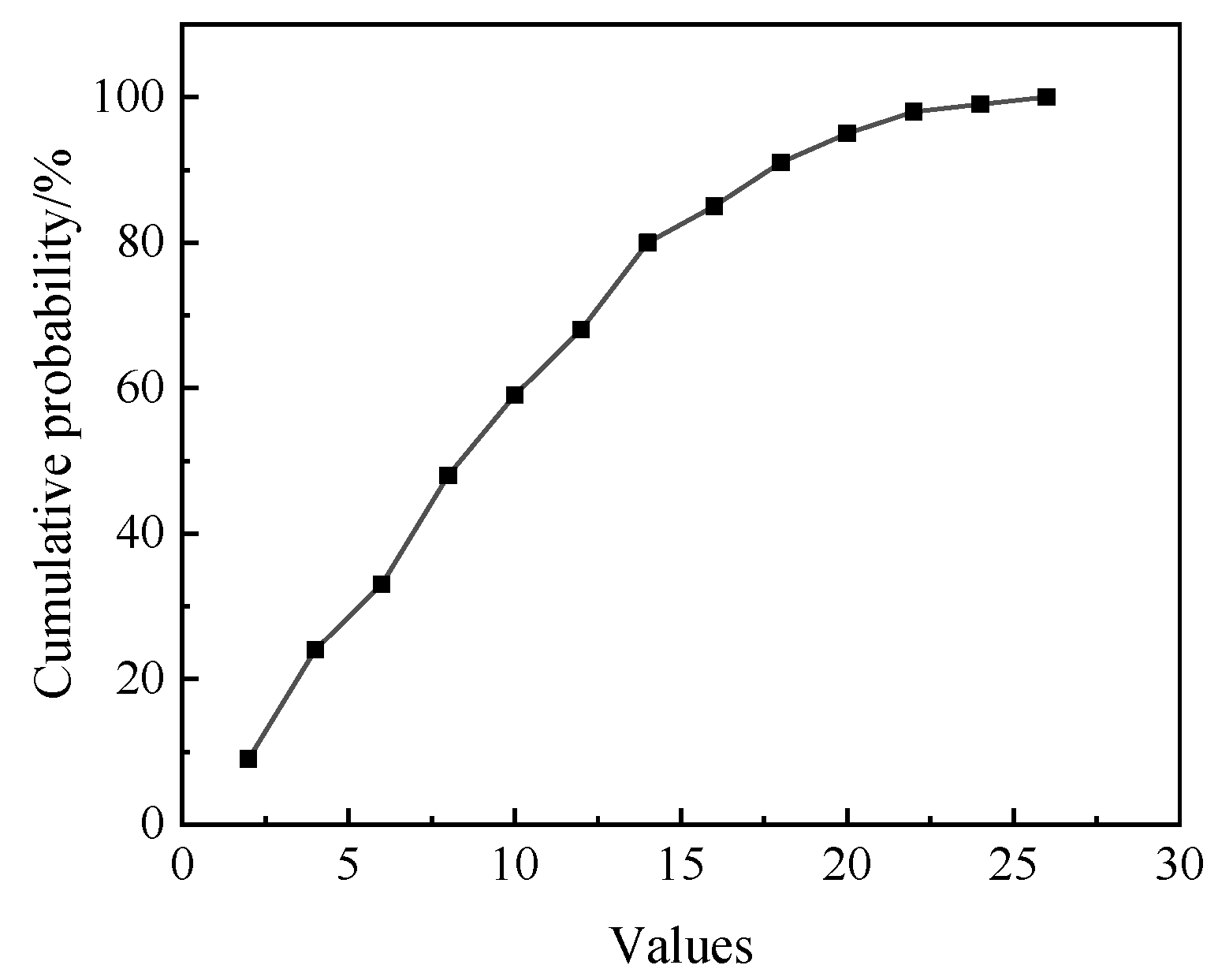
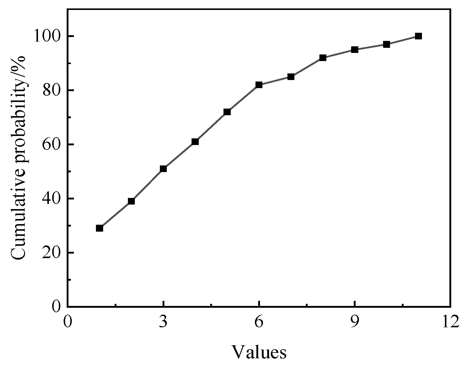
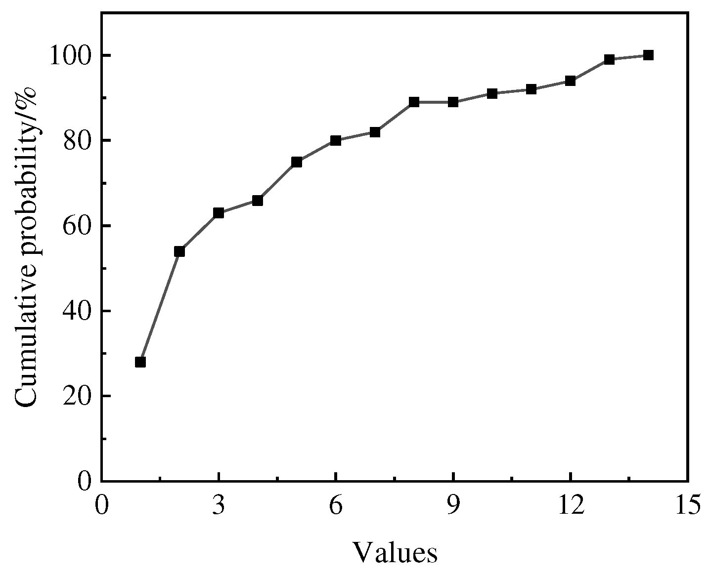
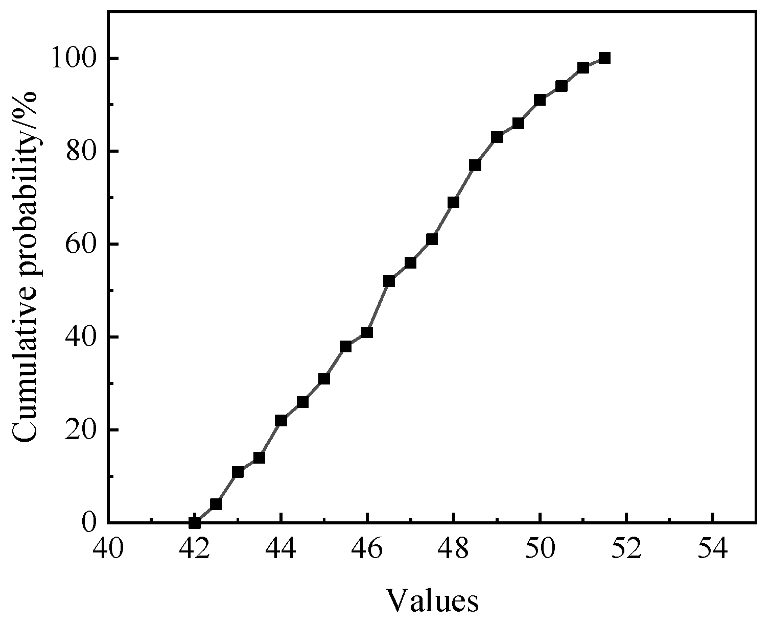
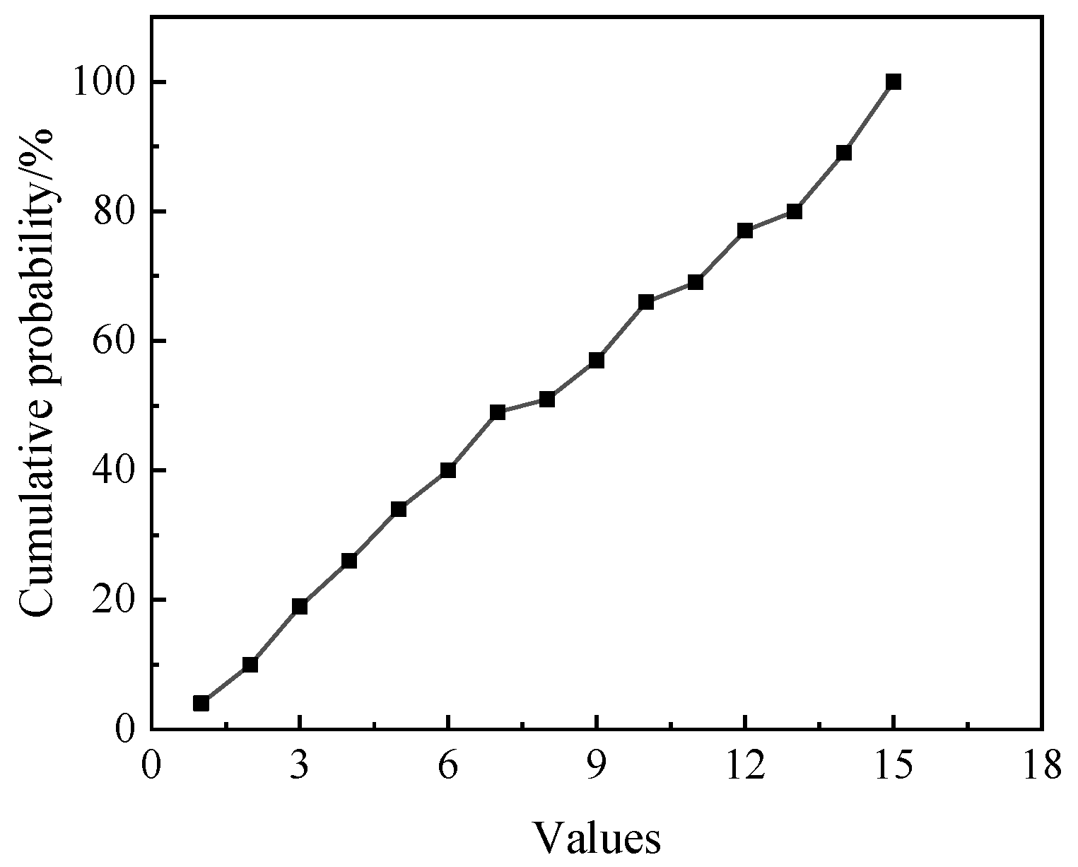
The eigenvalue estimation method from the earlier section is applied to the generated 100-size combinations. Figure 28, Figure 29, Figure 30, Figure 31, Figure 32, Figure 33, Figure 34, Figure 35, Figure 36 and Figure 37 present the EDFs obtained by fitting all 10 cognitive uncertainty variables using a probability box.

Taking the maximum cylinder pressure, the maximum cylinder temperature, and the indicated average effective pressure as the performance indexes, the EDF and eigenvalue estimation methods of each parameter obtained above are used to calculate the eigenvalue matrix of the function composed of 14 structural parameters, including the radius r of the front arc of the combustion chamber. The calculation results are shown in

Table 6. The calculated eigenvalues.

Structural Parameter	Performance Index
	Maximum Cylinder Pressure	Maximum Cylinder Temperature	Indicated Average Effective Pressure
r	2.1339	3.3178	2.5761
l	3.1528	4.7906	1.6218
h	4.6812	6.3345	3.7114
θ3	2.3218	8.2688	8.0427
R	2.8055	6.7792	4.1701
L	2.2952	4.3389	4.0759
H	14.2391	16.9644	14.4644
θ1	18.1673	18.1360	13.5508
θ2	16.6057	17.0970	14.9315
a	8.5642	9.3406	7.9712
b	16.8614	17.7883	8.6039
c	1.3363	1.2064	0.8551
q1	0.5012	0.7131	0.5182
q2	0.3877	0.9580	0.0224

. The larger the eigenvalues in the table, the greater the impact on the corresponding performance indicators.

Figure 38 illustrates the radar plot of each structural parameter’s impact on the performance index using the eigenvalue ratio. The coordinate axis indicates the influence percentage, and the larger structural parameters have a greater effect on the performance index.

From the figure, it can be seen that the effect of each structural parameter on the same performance index and that of the same structural parameter on different performance indexes is slightly different. However, whether the performance index is based on the maximum cylinder pressure, the maximum cylinder temperature, or the indicated average effective pressure, the three structural parameters that have the greatest influence on it are the angle θ2 between the rear bottom of the combustion chamber and the Y-Z plane, the distance b between the center of the top of the turbulent blade and the bottom of the combustion chamber, and the angle θ1 between the bottom of the middle of the combustion chamber and the Y-Z plane. The three structural parameters that have the least influence on the performance index are the spoiler width c, the radius of the excessive arc between the front of the combustion chamber and the middle of the combustion chamber q1, and the radius of the excessive arc between the middle of the combustion chamber and the rear of the combustion chamber q2. The vertical distance a between the spoiler and the rotor X-Z section and the distance b between the top center of the spoiler and the bottom edge of the combustion chamber have a greater influence on the maximum cylinder pressure and the maximum cylinder temperature but have a smaller influence on the indicated average effective pressure.

Through the above chart, the main structural parameter combination can be obtained, which is composed of the angle θ1 between the bottom edge of the middle part of the combustion chamber and the Y-Z plane, the distance b between the center of the spoiler top and the bottom edge of the combustion chamber, the angle θ2 between the bottom edge of the rear part of the combustion chamber and the Y-Z plane, the distance H between the bottom of the middle and rear part of the combustion chamber at the X-Z section of the rotor and the center of gravity of the rotor, the vertical distance a between the spoiler and the X-Z section of the rotor, the angle θ3 between the bottom edge of the front part of the combustion chamber and the Y-Z plane, the radius R of the middle and rear part of the combustion chamber, and the distance h between the bottom of the front part of the combustion chamber at the X-Z section of the rotor. The influence of this parameter combination on the maximum cylinder pressure, the maximum cylinder temperature, and the indicated average effective pressure is 89.5728%, 86.7924%, and 89.0677%, respectively. The influence of structural parameters such as the bottom edge length l of the front part of the combustion chamber, the bottom edge length L of the middle and rear part of the combustion chamber, the arc radius r of the front part of the combustion chamber, the width c of the spoiler, the excessive arc radius q2 between the middle part of the combustion chamber and the rear part of the combustion chamber, and the excessive arc radius q1 between the front part of the combustion chamber and the middle part of the combustion chamber is small and can be ignored in the study of combustion chamber structure optimization. This is consistent with the current research trend regarding the structural parameters of the combustion chamber of the rotary engine. On this basis, three structural parameters can be obtained, which are the angle θ2 between the bottom edge of the combustion chamber and the Y-Z plane, the distance H between the bottom of the middle and rear section of the combustion chamber at the X-Z section of the rotor and the center of gravity of the rotor, and the angle θ1 between the bottom edge of the middle of the combustion chamber and the Y-Z plane. These three structural parameters should be used as important structural parameters for the study of the combustion chamber structure of the rotary engine. These three parameters have a great influence on each performance index, and the influence on the maximum cylinder pressure, the maximum cylinder temperature, and the indicated average effective pressure are 52.1109%, 45.9847%, and 50.4569%, respectively.

Since the design of the combustion chamber structure demands a variety of requirements, including compression ratio, process, and structure, after optimizing the above structural parameters that have the greatest impact on performance, it is necessary to change some structural parameters at the same time to make them meet many requirements, including compression ratio. It can be seen from the above charts that the three structural parameters, such as the length l of the front bottom of the combustion chamber, the length L of the rear bottom of the combustion chamber, and the radius r of the front arc of the combustion chamber, have a small proportion of influence on each performance index. The influence of these three parameters on the maximum cylinder pressure, the maximum cylinder temperature, and the indicated mean effective pressure is 8.7753%, 13.7104%, and 11.5934%, respectively, and the range of parameters is large. Because the change in parameters has a great influence on the compression ratio, process, and strength requirements, the above three structural parameters can be used as adjustable structural parameters in the study of combustion chamber structure optimization. When the main structural parameters are determined, the adjustable structural parameters are adjusted to make the combustion chamber meet many requirements, including compression ratio, process, and structure.

5. Conclusions

In order to reduce the dimension in the optimization process of the combustion chamber structure of the rotary engine and clarify the optimization priority and direction, this paper proposes a dimension reduction method for the structural parameters of the combustion chamber of the rotary engine based on the AS, referring to the probability box and EDF. The main research contents of this paper are as follows:

• By analyzing the generation process of the active subspace and the composition of rotor structure parameters, based on active subspace, combined with the probability box and EDF, a dimension reduction method for rotary engine combustion chamber structure parameters is proposed, and the accuracy of the method is verified. The results show that the deviation between the calculated eigenvalues and the actual eigenvalues is only 1.2931%, and the estimation accuracy is high, which can be used for eigenvalue calculation and parameter dimension reduction of high-dimensional mixed uncertainty problems.
• Using the dimension reduction method proposed above, the dimension combination composed of 14 structural parameters is reduced to an important structural parameter composed of 8 structural parameters, including θ1, b, θ2, H, a, θ3, R, and h. The effects of the above eight structural parameters on the maximum cylinder pressure, the maximum cylinder temperature, and the indicated mean effective pressure are 89.5728%, 86.7924%, and 89.0677%, respectively.
• On this basis, three main structural parameters, with the influence of θ2 accounting for more than 45%, are obtained. And three adjustable structural parameters, including l, are obtained. The influence of the latter on the total proportion of each performance index is small, and the influence on the maximum cylinder pressure, the maximum cylinder temperature, and the indicated average effective pressure is 8.7753%, 13.7104%, and 11.5934%, respectively. Moreover, the change in parameters has a great influence on the compression ratio, process, and strength requirements. Therefore, the above three structural parameters can be used as adjustable structural parameters in the optimization of combustion chamber structure. When the main structural parameters are determined, the adjustable structural parameters are adjusted to make the combustion chamber meet many requirements, including compression ratio, process, and structure.

In the future, based on the research in this paper, the research group will deeply study the influencing law of combustion chamber structure parameters on engine performance and quantitatively analyze it, hoping to obtain the influence proportions of different combustion chamber structure parameters and different levels of the same structure parameters on engine performance. Furthermore, the dimension reduction method based on AS proposed in this paper will be applied to the research of other structure or control parameters of rotary engines, which provides a reference and basis for further improving the performance of rotary engines and broadening the application field of rotary engines.

References

1. Wang, S. The Status of the Power Plants for UAVs in China. Aerosp. Power 2019, 2, 9–12. [Google Scholar]
2. Dong, Y.; Huang, M.; Li, R. Overview of the Development of General Aviation Engines. J. Xi’an Aeronaut. Univ. 2017, 35, 8–13. [Google Scholar]
3. Yin, Z.; Li, S.; Li, G. Current State and Development of the Unmanned Aerial Vehicle Power plant. Aeroengine 2007, 33, 10–15. [Google Scholar]
4. Lu, D.; Zheng, J.; Hu, C.; Bian, S. Research on the development status of general aviation piston engine. Intern. Combust. Engine Parts 2019, 8, 64–66. [Google Scholar]
5. Feng, G.; Zhou, M. Assessment of heavy fuel aircraft piston engine type. J. Tsinghua Univ. 2016, 56, 1114–1121. [Google Scholar]
6. Jiao, H.; Liu, J.; Zou, R.; Wang, N. Combined influence of ignition chamber volume and spark plug channel diameter on the performance of small-scale natural gas Wankel rotary engine. Eng. Appl. Comput. Fluid Mech. 2021, 15, 1775–1791. [Google Scholar] [CrossRef]
7. Kong, X.; Liu, H. Research Progress of Key Technologies of Aviation Piston Engine for UAV. Small Intern. Combust. Engine Veh. Tech. 2021, 50, 79–87. [Google Scholar]
8. Johar, T.; Hsieh, C.F. Design Challenges in Hydrogen-Fueled Rotary Engine-A Review. Energies 2023, 16, 607. [Google Scholar] [CrossRef]
9. Wu, S. Research on Technical Characteristics and Application of Unmanned Aerial Vehicle Power Unit. Shanghai Energy Sav. 2022, 1536–1540. [Google Scholar]
10. Wang, X.; Liu, J. GE Aerospace’s Roadmap for Next-Generation Aerospace Power Technology. Aerosp. Power 2023, 24–27. [Google Scholar]
11. Li, H.; Sun, F. The Application Development and Key Technologies of Wankel engine. Small Intern. Combust. Engine Veh. 2023, 52, 68–74. [Google Scholar]
12. Kotsiopoulos, P.; Yfantis, E.; Lois, E.; Hountalas, D. Diesel and JP-8 fuel performance on a Petter AVI diesel engine. In Proceedings of the 39th Aerospace Sciences Meeting and Exhibit (AIAA), Reno, NV, USA, 8–11 January 2001. [Google Scholar] [CrossRef]
13. Dutczak, J. Heavy fuel engines. Combust. Engines 2015, 163, 34–46. [Google Scholar] [CrossRef]
14. Wu, H.; Wang, L.L.; Wu, Y.; Sun, B.; Zhao, Z.; Liu, F. Spray performance of air-assisted kerosene injection in a constant volume chamber under various in-cylinder GDI engine conditions. Appl. Therm. Eng. 2019, 150, 762–769. [Google Scholar] [CrossRef]
15. Li, Z. Simulation Analys is on Cooperative Control of Ignition and Knock of Light-Weight, Spark Ignition, Heavy Oil Aeroengine. Master’s Thesis, Beijing Jiao Tong University, Beijing, China, 2016. [Google Scholar]
16. Wang, Z. Experimental Study on Performance of 15kW Two-Stroke Ignited PFI Kerosene Piston Engine. Master’s Thesis, Nanjing University of Aeronautics and Astronautics, Nanjing, China, 2018. [Google Scholar]
17. Attard, W.P.; Blaxill, H.; Anderson, E.K.; Litke, P. Knock limit extension with a gasoline fueled pre -chamber jet igniter in a modern vehicle powertrain. SAE Int. J. Engines 2012, 5, 1201–1215. [Google Scholar] [CrossRef]
18. Wang, C.Y.; Zhang, F.J.; Wang, E.H.; Yu, C.; Gao, H.; Liu, B.; Zhao, Z.; Zhao, C. Experimental study on knock suppression of spark -ignition engine fueled with kerosene via water injection. Appl. Energy 2019, 242, 248–259. [Google Scholar] [CrossRef]
19. Chen, L.F.; Raza, M.; Xiao, J.H. Combustion analysis of an aviation compression ignition engine burning pentanol kerosene blends under different injection timings. Energy Fuel 2017, 31, 9429–9437. [Google Scholar] [CrossRef]
20. Ning, L.; Duan, Q.M.; Wei, Y.H.; Zhang, X.; Yu, K.; Yang, B.; Zeng, K. Effects of injection timing and compression ratio on the combustion performance and emissions of a two -stroke DISI engine fuelled with aviation kerosene. Appl. Therm. Eng. 2019, 161, 114–124. [Google Scholar]
21. Lu, Y.; Pan, J.F.; Fan, B.W.; Otchere, P.; Chen, W.; Cheng, B. Research on the application of aviation kerosene in a direct injection wankel engine -Part 1: Fundamental spray characteristics and optimized injection strategies. Energy Convers. Manag. 2019, 195, 519–532. [Google Scholar] [CrossRef]
22. Yang, J.; Ji, C.; Wang, S.; Wang, D.; Ma, Z.; Zhang, B. Numerical investigation on the mixture formation and combustion processes of a gasoline wankel engine with direct injected hydrogen enrichment. Appl. Energy 2018, 224, 34–41. [Google Scholar] [CrossRef]
23. Cao, B.W.; Liu, J.X. Design and optimization of orifice plates in the air-assisted kerosene injection system applied in the wankel rotary engine. Proc. Inst. Mech. Eng. Part C-J. Mech. Eng. Sci. 2023, 237, 2945–2953. [Google Scholar] [CrossRef]
24. Zhao, Y.; Deng, X.; Feng, Z.; Zhu, R.; Su, X. Effects of Combustion Chamber Pit Shape on Combustion Process for Gasoline Wankel engine. Veh. Engine 2022, 40–46. [Google Scholar]
25. Kuo, C.H.; Ma, H.L.; Chen, C.C. Chamber contour design and compression flow calculations of wankel engine. J. CCIT 2010, 39, 35–50. [Google Scholar]
26. Tartakovsky, L.; Baibikov, V.; Gutman, M.; Veinblat, M.; Reif, J. Simulation of Wankel engine performance using commercial software for piston engines. In Proceedings of the 2012 Small Engine Technology Conference & Exhibition, Madison, WI, USA, 16–18 October 2012. SAE Technical Paper 2012–32-0098. [Google Scholar]
27. Jeng, D.Z.; Hsieh, M.J.; Lee, C.C.; Han, Y. The numerical investigation on the performance of wankel engine with leakage, different fuels and recess sizes. In Proceedings of the JSAE/SAE 2013 Small Engine Technology Conference, Taipei, Taiwan, 8–10 October 2013. SAE Technical Paper 2013–32-9160. [Google Scholar]
28. Wei, F.B.; Feng, P.J.; Xian, L.Y.; Rui, C.; Di, W.U. Effect of pocket location on combustion process in natural gas-fueled wankel engine. Appl. Mech. Mater. 2013, 316–317, 73–79. [Google Scholar] [CrossRef]
29. Fan, B.W.; Pan, J.F.; Pan, Z.H.; Tang, A.K.; Zhu, Y.J.; Xue, H. Effects of pocket shape and ignition slot locations on the combustion processes of a wankel engine fueled with natural gas. Appl. Therm. Eng. 2015, 89, 11–27. [Google Scholar] [CrossRef]
30. Ji, C.W.; Su, T.; Zhang, S.F.; Yu, M.; Cong, X. Effect of hydrogen addition on combustion and emissions performance of a gasoline wankel engine at part load and stoichiometric conditions. Energy Convers. Manag. 2016, 121, 272–280. [Google Scholar] [CrossRef]
31. Amrouche, F.; Varnhagen, S.; Erickson, P.A.; Park, J. An experimental study of a hydrogen-enriched ethanol fueled Wankel wankel engine at ultra lean and full load conditions. Energy Convers. Manag. 2016, 123, 174–184. [Google Scholar] [CrossRef]
32. Su, T.; Ji, C.; Wang, S.; Shi, L.; Cong, X. Effect of ignition timing on performance if a hydrogen-enriched n-butanol wankel engine at lean condition. Energy Convers. Manag. 2018, 161, 27–34. [Google Scholar] [CrossRef]
33. Chen, W.; Pan, J.; Fan, B.; Liu, Y.; Peter, O. Effect of injection strategy on fuel-air mixing and combustion process in a direct injection diesel wankel engine (DI-DRE). Energy Convers. Manag. 2017, 154, 68–80. [Google Scholar] [CrossRef]
34. Shi, C.; Zhang, P.; Ji, C. Understanding the role of turbulence-induced blade configuration in improving combustion process for hydrogen-enriched wankel engine. Fuel 2022, 319, 123807. [Google Scholar] [CrossRef]
35. Bienner, A.; Gloerfelt, X.; Cinnella, P. Leading-Edge Effects on Freestream Turbulence Induced Transition of an Organic Vapor. Flow Turbul. Combust. 2024, 224, 345–373. [Google Scholar] [CrossRef]
36. Li, M.; Hamel, J.; Azarm, S. Optimal uncertainty reduction for multi-disciplinary multi-output systems using sensitivity analysis. Struct. Multidiscip. Optim. 2010, 40, 77–96. [Google Scholar] [CrossRef]
37. Davey, K.; Sadeghi, H.; Darvizeh, R. The theory of scaling. Contin. Mech. Thermodyn. 2023, 35, 471–496. [Google Scholar] [CrossRef]
38. Jolliffe, I. Principal Component Analysis; Wiley Online Library: Hoboken, NJ, USA, 2002. [Google Scholar]
39. Duda, R.O.; Hart, P.E.; Stork, D.G. Pattern Classification; John Wiley & Sons: Hoboken, NJ, USA, 2012. [Google Scholar]
40. Wang, J. Geometric Structure of High-Dimensional Data and Dimensionality Reduction; Springer: Berlin/Heidelberg, Germany, 2012. [Google Scholar]
41. Schölkopf, B.; Smola, A.; Müller, K.-R. Nonlinear component analysis as a kernel eigenvalue problem. Neural Comput. 1998, 10, 1299–1319. [Google Scholar] [CrossRef]
42. Roweis, S.T.; Saul, L.K. Nonlinear dimensionality reduction by locally linear embedding. Science 2000, 290, 2323–2326. [Google Scholar] [CrossRef]
43. Donoho, D.L.; Grimes, C. Hessian eigenmaps: Locally linear embedding techniques for high-dimensional data. Proc. Natl. Acad. Sci. USA 2003, 100, 5591–5596. [Google Scholar] [CrossRef]
44. Belkin, M.; Niyogi, P. Laplacian Eigenmaps for Dimensionality Reduction and Data Representation. Neural Comput. 2003, 15, 1373–1396. [Google Scholar] [CrossRef]
45. Constantine, P.G. Active Subspaces: Emerging Ideas for Dimension Reduction in Parameter Studies; SIAM: Philadelphia, PA, USA, 2015. [Google Scholar]
46. Scott, D.W. The Curse of Dimensionality and Dimension Reduction. In Multivariate Density Estimation; Wiley: Hoboken, NJ, USA, 2008. [Google Scholar]
47. Wang, B.X.; Huang, X.Z.; Chang, M.X. Regional reliability sensitivity analysis based on dimension reduction technique. Probabilistic Eng. Mech. 2023, 74, 1394–1419. [Google Scholar] [CrossRef]
48. Russi, T.M. Uncertainty Quantification with Experimental Data and Complex System Models. Ph.D. Thesis, University of California, Berkeley, CA, USA, 2010. [Google Scholar]
49. Stewart, G.W. Error and perturbation bounds for subspaces associated with certain eigenvalue problems. SIAM Rev. 1973, 15, 727–764. [Google Scholar] [CrossRef]
50. Davey, K.; Abd Malek, M.I.; Ali, Z.; Sadeghi, H.; Darvizeh, R. The theory of scaled electromechanics. Int. J. Eng. Sci. 2024, 203, 1041–1068. [Google Scholar] [CrossRef]
51. Fujimori, K.; Goto, Y.; Liu, Y.; Taniguchi, M. Sparse principal component analysis for high-dimensional stationary time series. Scand. J. Stat. 2023, 50, 1953–1983. [Google Scholar] [CrossRef]
52. Wang, M.; Lu, Y.; Pan, W. An improved pattern-based prediction model for a class of industrial processes. Trans. Inst. Meas. Control. 2022, 44, 1410–1423. [Google Scholar] [CrossRef]
53. Chib, S.; Greenberg, E. Understanding the metropolis-hastings algorithm. Am. Stat. 1995, 49, 327–335. [Google Scholar] [CrossRef]
54. Ray, T. Golinski’s speed reducer problem revisited. AIAA J. 2003, 41, 556–558. [Google Scholar] [CrossRef]
55. Allen, M.; Maute, K. Reliability-based design optimization of aeroelastic structures. Struct. And. Multidiscip. Optim. 2004, 27, 228–242. [Google Scholar] [CrossRef]
56. Lillacci, G.; Khammash, M. A distribution-matching method for parameter estimation and model selection in computational biology. Int. J. Robust Nonlinear Control 2012, 22, 1065–1081. [Google Scholar] [CrossRef]
57. Seshadri, P.; Constantine, P.; Iaccarino, G.; Parks, G. Aggressive design: A density-matching approach for optimization under uncertainty. arXiv 2014, arXiv:1409.7089. [Google Scholar]
58. Ferson, S.; Kreinovich, V.; Ginzburg, L.; Myers, D.S.; Sentz, K. Constructing Probability Boxes and Dempster-Shafer Structures; SAND2003-4015; Sandia National Laboratories: Albuquerque, NM, USA, 2003. [Google Scholar]
59. Yang, X. Research on Highly Efficient and Precise Methods for Reliability Analysis with Epistemic Uncertainties. Master’s Thesis, Northwestern Polytechnical University, Xi’an, China, 2016. [Google Scholar]
60. Huang, X.; Wang, Q.; Ding, J. Faculty of Information Engineering and Automation: Index Uncertainty Modeling in Grid Planning Based on Probability Box Theory. Inf. Control 2016, 45, 272–277. [Google Scholar]
61. Ferson, S.; Tucker, W.T. Sensitivity in Risk Analyses with Uncertain Numbers; Sandia National Laboratories: Albuquerque, NM, USA, 2006; pp. 156–159. [Google Scholar]
62. Crespo, L.G.; Kenny, S.P.; Giesy, D.P. Reliability analysis of polynomial systems subject to p-box uncertainties. Mech. Syst. Signal Process. 2013, 37, 121–136. [Google Scholar] [CrossRef]
63. Beer, M.; Ferson, S.; Kreinovich, V. Imprecise probabilities in engineering analyses. Mech. Syst. Signal Process. 2013, 37, 4–29. [Google Scholar] [CrossRef]
64. Jiao, H.; Ye, X.; Zou, R.; Wang, N.; Liu, J. Comparative study on ignition and combustion between conventional spark-ignition method and near-wall surface ignition method for small-scale Wankel rotary engine. Energy 2022, 255, 1049–1072. [Google Scholar] [CrossRef]
65. Zou, R.; Liu, J.; Jiao, H.; Zhao, J.; Wang, N. Combined effect of intake angle and chamber structure on flow field and combustion process in a small-scaled rotary engine. Appl. Therm. Eng. 2022, 203, 1497–1521. [Google Scholar] [CrossRef]
66. Hege, J. The Wankel Wankel Engine: A History; McFarland and Company Inc.: Jefferson, NC, USA, 2006. [Google Scholar]
67. Wladyslaw, M. Modelling and Simulation of Working Processes in Wankel Engine with Direct Hydrogen Injection System. Combust. Engines 2015, 161, 42–52. [Google Scholar]
68. Peden, M. Study of Direct Injection Limitations on a Wankel Engine. Master’s Thesis, University of Bath, Bath, UK, 2017. [Google Scholar]
69. Wendeker, M.; Grabowski, L.; Pietrykowski, K.; Margryta, P. Phenomenological Model of a Wankel Engine; Lublin University of Technology: Lublin, Poland, 2012. [Google Scholar]
70. Tomlinson, A. Modelling of Wankel Engine Performance in Commercial Piston Engine Software. Master’s Thesis, University of Bath, Bath, UK, 2016. [Google Scholar]
71. Georgios, Z. Mathematical and Numerical Modelling of Flow and Combustion Processes in a Spark Ignition Engine. Master’s Thesis, Department of Applied Mathematics, University of Wisconsin, Madison, WI, USA, 2005. [Google Scholar]
Figure 1. Wankel engine combustion chamber structure.
Processes 12 02238 g001
Figure 2. Variable comparison table.
Processes 12 02238 g002
Figure 3. Combustion chamber dimensions. (a) A-A section size. (b) B-B section size. (c) C-C section angle. (d) C-C section size.
Processes 12 02238 g003
Figure 4. Distribution of the arc radius (r) at the leading edge of the combustion chamber. (a) Distribution conditions. (b) Distribution probability.
Processes 12 02238 g004
Figure 5. Distribution of the length (l) at the leading bottom edge of the combustion chamber. (a) Distribution conditions. (b) Distribution probability.
Processes 12 02238 g005
Figure 6. Distribution of the distance (h) from the front section bottom of the combustion chamber to the rotor’s center of gravity in the x-z plane. (a) Distribution conditions. (b) Distribution probability.
Processes 12 02238 g006
Figure 7. Distribution of the angle (θ3) between the leading bottom edge of the combustion chamber and the y-z plane. (a) Distribution conditions. (b) Distribution probability.
Processes 12 02238 g007
Figure 8. Distribution of the length (R) at the trailing bottom of the combustion chamber. (a) Distribution conditions. (b) Distribution probability.
Processes 12 02238 g008
Figure 9. Distribution of the length (L) at the trailing bottom of the combustion chamber. (a) Distribution conditions. (b) Distribution probability.
Processes 12 02238 g009
Figure 10. Distribution of the distance (H) from the trailing chamber bottom to the rotor’s center of gravity in the x-z plane. (a) Distribution conditions. (b) Distribution probability.
Processes 12 02238 g010
Figure 11. Distribution of the angle (θ1) between the combustion chamber’s middle bottom edge and the y-z plane. (a) Distribution conditions. (b) Distribution probability.
Processes 12 02238 g011
Figure 12. Distribution of the angle (θ2) between the trailing bottom of the combustion chamber and the y-z plane. (a) Distribution conditions. (b) Distribution probability.
Processes 12 02238 g012
Figure 13. Distribution of the vertical distance (a) between the spoiler plate and the rotor x-z section. (a) Distribution conditions. (b) Distribution probability.
Processes 12 02238 g013
Figure 14. Distribution of the distance (b) from the spoiler top center to the chamber bottom edge. (a) Distribution conditions. (b) Distribution probability.
Processes 12 02238 g014
Figure 15. The distribution of the spoiler plate width (c). (a) Distribution conditions. (b) Distribution probability.
Processes 12 02238 g015
Figure 16. Distribution of the excessive arc radius (q1) between the leading and middle chamber sections. (a) Distribution conditions. (b) Distribution probability.
Processes 12 02238 g016
Figure 17. Distribution of the excessive arc radius (q2) between the middle and trailing chamber sections. (a) Distribution conditions. (b) Distribution probability.
Processes 12 02238 g017
Figure 18. Eigenvalue estimation of the mixed uncertainty active subspace using the EDF and probability box.
Processes 12 02238 g018
Figure 19. EDF distribution.
Processes 12 02238 g019
Figure 20. Probability box.
Processes 12 02238 g020
Figure 21. Probability box and structure.
Processes 12 02238 g021
Figure 22. Distribution of the independent variable x 2 . (a) Distribution conditions. (b) Distribution probability.
Processes 12 02238 g022
Figure 23. Fit EDF depicting the EDF fitted using the probability box.
Processes 12 02238 g023
Figure 24. Three-dimensional model. (a) Cylinder fluid domain. (b) Rotor entity.
Processes 12 02238 g024
Figure 25. The cylinder pressure change curve under different grid numbers. (a) Ignition state. (b) Non-ignition state.
Processes 12 02238 g025
Figure 26. Rotor engine computational grid.
Processes 12 02238 g026
Figure 27. Performance index. (a) Maximum cylinder pressure. (b) Maximum cylinder temperature.
Processes 12 02238 g027aProcesses 12 02238 g027b
Figure 28. EDF fitting of the arc radius r in the combustion chamber.
Processes 12 02238 g028
Figure 29. EDF fitting for the combustion chamber leading bottom length l.
Processes 12 02238 g029
Figure 30. EDF fitting for the distance (h) between the combustion chamber bottom and the rotor’s center of gravity in the x-z plane.
Processes 12 02238 g030
Figure 31. EDF fitting for the angle (θ3) between the bottom edge of the combustion chamber’s leading section and the y-z plane.
Processes 12 02238 g031
Figure 32. EDF fitting of the arc radius (R) in the combustion chamber’s trailing section.
Processes 12 02238 g032
Figure 33. EDF fitting of the trailing bottom edge length (L) of the combustion chamber.
Processes 12 02238 g033
Figure 34. EDF fitting of the distance (H) from the combustion chamber’s trailing bottom to the rotor’s center of gravity in the x-z plane.
Processes 12 02238 g034
Figure 35. EDF fitting of the angle (θ1) between the bottom edge of the combustion chamber’s middle section and the y-z plane.
Processes 12 02238 g035
Figure 36. EDF fitting of the angle (θ2) between the rear bottom edge of the combustion chamber and the y-z plane.
Processes 12 02238 g036
Figure 37. EDF fitting of the distance (b) between the center of the spoiler plate top and the bottom of the combustion chamber.
Processes 12 02238 g037
Figure 38. Impact of structural parameters on various performance metrics. (a) Impact of numerous structural parameters on maximum cylinder pressure. (b) Effect of different structural parameters on peak cylinder temperature. (c) Effect of each structural parameter on the indicated mean effective pressure.
Processes 12 02238 g038