Abstract
IoT sensors in oilfields gather real-time data sequences from oil wells. Accurate trend predictions of these data are crucial for production optimization and failure forecasting. However, oil well time series data exhibit strong nonlinearity, requiring not only precise trend prediction but also the estimation of uncertainty intervals. This paper first proposed a data denoising method based on Variational Mode Decomposition (VMD) and Long Short-Term Memory (LSTM) to reduce the noise present in oil well time series data. Subsequently, an SDMI loss function was introduced, combining the respective advantages of Soft Dynamic Time Warping and Mean Squared Error (MSE). The loss function additionally accepts the upper and lower bounds of the uncertainty prediction interval as input and is optimized with the prediction sequence. By predicting the data of the next 48 data points, the prediction results using the SDMI loss function and the existing three common loss functions are compared on multiple data sets. The prediction results before and after data denoising are compared and the results of predicting the uncertainty interval are shown. The experimental results demonstrate that the average coverage rate of the predicted uncertainty intervals across data from seven wells is 81.4%, and the prediction results accurately reflect the trends in real data.
1. Introduction
With the construction of the Internet of Things (IoT) in oilfields [1,2,3], a large number of sensors have been installed on oil wells, enabling the real-time monitoring of oil well operational status data. On this basis, if accurate prediction of oil well time series data can be achieved, it will play a crucial role in improving production efficiency, reducing costs and risks, assisting production decision-making, extending the service life of oil wells, and strengthening enterprise management. However, due to the influence of multiple factors such as geological structures and the nature of oil and gas reservoirs, as well as equipment failures, sensor malfunctions, or data transmission errors, oil well time series data exhibit highly nonlinear characteristics. Additionally, oil well time series data often contain noise and missing values, further increasing the complexity of the data and making it difficult to accurately predict long-term future data trends.
Currently, researchers in the petroleum field have proposed numerous methods for time series prediction, but these methods suffer from several issues. Firstly, existing noise reduction techniques include Kalman Filtering, EMD [4], VMD [5], and several others. However, these noise reduction methods may fail to capture the long-term dependencies in oil well time series data, resulting in unsatisfactory noise reduction effects. Secondly, the loss functions commonly employed in these methods, such as MSE (Mean Squared Error) and RMSE (Root Mean Squared Error), have limitations. Time series prediction aims to forecast a sequence of future data points rather than a single future data point. Point-to-point error metrics like MSE may not be appropriate for time series prediction tasks because MSE fails to account for the dynamic changes in time series data over time, such as time delays. For instance, if two highly similar data sequences exhibit a time delay, their MSE error could be significant even though they appear very similar. Furthermore, these methods often predict certain values, but in fact, due to the influence of many complex situations, the changing trend of oil well data is uncertain, and there are many random factors. Therefore, it is reasonable to not only predict a certain value but also provide an additional uncertainty interval, offering a range for data variation. In addition, due to the existence of noise, a method suitable for oil well data noise reduction is needed, but there is a lack of research on oil well data noise reduction methods. To address these issues, it decides to improve upon existing methods in terms of both the loss function and data noise reduction methods.
For the issue of data noise reduction, a method combining the VMD algorithm with an LSTM prediction model is proposed. The aim of combining these two techniques is to more accurately uncover the long-term dependencies in oil well time series data. To address the issues related to the loss function and uncertainty prediction interval, a hybrid loss function named SDMI is introduced. SDMI integrates Soft-DTW and MSE for time series prediction and incorporates loss functions associated with the coverage and width of the prediction interval to facilitate uncertainty interval prediction.
The main contributions of this paper are as follows:
- A novel loss function is proposed that accepts four inputs (predicted sequence, upper bound of prediction interval, lower bound of prediction interval, and true sequence). It can take into account the similarity and time correspondence between prediction time series and real value time series and can optimize the predicted sequence and the upper and lower bounds of the uncertainty prediction interval simultaneously.
- A new method for time series data noise reduction is proposed that integrates the VMD algorithm with the LSTM model. This approach is characterized by its ease of implementation, rapid noise reduction process, and wide applicability.
- Experiments are conducted on multiple datasets from an oilfield company, utilizing the Informer-based time series prediction model to forecast the changing trends of the next 48 data values. By comparing existing data noise reduction methods and loss functions, the superiority of the proposed method is validated.
The remaining parts of this paper are organized as follows: Section 2 reviews related work; Section 3 introduces the proposed SDMI loss function and the proposed data noise reduction method; Section 4 presents the datasets and experimental setups; Section 5 analyzes the experimental results and discusses them; Section 6 provides a summary.
2. Related Works
This section introduces current related research from four aspects: time series prediction models, Dynamic Time Warping (DTW) loss function, uncertainty prediction, and data denoising.
2.1. Time Series Prediction Model
Currently, numerous models have been employed for time series prediction tasks, such as ARIMA, RNN, LSTM, and Transformer. In the field of petroleum engineering, there has also been extensive research, including well production forecasting [6,7], oil price prediction [8,9,10], and fault prediction [11,12,13,14,15]. Recent studies primarily focus on methods that combine algorithms like LSTM with self-attention mechanisms. For instance, Zhou et al. proposed a method for spatiotemporal feature extraction from shale oil production data based on Convolutional Neural Networks (CNN) and Bidirectional Gated Recurrent Units (BiGRU) combined with an attention mechanism for production prediction [16]. Pan et al. introduced a well production prediction method that integrates CNN-LSTM with a self-attention mechanism [17]. Leng et al. presented a dynamic liquid level prediction method for oil wells that combines LSTM, an attention mechanism, and the Whale Optimization Algorithm (WOA) [18]. These researchers have all validated the accuracy of their proposed methods through experiments, demonstrating the effectiveness of neural network algorithms in time series prediction tasks within the petroleum industry.
Building upon Transformer, the Informer has been derived, offering certain advantages over Transformer in terms of long sequence processing capability, computational efficiency, and prediction accuracy. Compared to other methods, such as traditional machine learning and artificial neural networks, the Informer model demonstrates more outstanding capabilities in handling long sequences, higher computational efficiency, and more accurate prediction accuracy in time series forecasting tasks. Therefore, in this paper, the Informer model is chosen as the prediction model.
2.2. Dynamic Time Warping
The DTW algorithm differs from algorithms like MSE in that it takes into account the overall shape and temporal relationships of time series, and it can measure the similarity between two sequences of different lengths. This makes it useful for addressing situations where MSE may sometimes fail to predict the overall pattern or trend of a time series. However, the DTW algorithm itself is discrete and cannot be directly used as a loss function. Soft-DTW [19], on the other hand, modifies the DTW algorithm to solve this problem.
In current research, the DTW algorithm and the Soft-DTW algorithm are primarily used for time series recognition, retrieval, and clustering. Li et al. proposed a spherical-DTW algorithm to find the optimal match between test trajectories and training trajectories during the retrieval process [20]. Pan et al. employed a data clustering method based on DTW and K-medoids in their paper and validated its effectiveness on a sequence dataset comprising 377 operation cycles from the TBM tunneling project in Singapore [21]. Similar research by Li et al. also employed a clustering method based on Soft-DTW-K-medoids [22]. Ding et al. verified the feasibility of using the DTW algorithm to monitor disturbances in the Minjiang River basin [23]. Zhu et al. utilized a clustering method based on DTW to identify different degradation patterns of shield tunnels and employed LSTM to predict their performance [24].
Although the above studies did not directly use the DTW algorithm as a loss function for time series prediction, it was demonstrated that the DTW algorithm can more effectively measure the similarity between two time series. This validates the feasibility of using the Soft-DTW algorithm as a loss function for time series prediction models. Furthermore, this paper addresses the potential issue of time lag in time series prediction when using the DTW algorithm by combining it with the MSE algorithm, thereby further improving prediction accuracy.
2.3. Uncertainty Prediction
Due to the need to predict a significant amount of future data in oil well time series forecasting tasks, which are inevitably influenced by numerous uncertain factors, it is essential to consider the possibility interval of data variation in predictions. Currently, there are numerous methods for uncertainty prediction. Wang et al. modeled and predicted uncertainties in time series data using Bayesian networks and validated their effectiveness on 14 public time series datasets [25]. However, this method suffers from computational complexity, long time consumption, and dependence on data quality. In the research by Cartagena et al., a multivariate fuzzy prediction interval method was proposed to enhance prediction robustness [26], but it did not address the issue of computational complexity. Regarding the study of prediction intervals, Guan et al. introduced a method for predicting the upper and lower bounds of uncertainty intervals [27], but it did not take into account the necessity of predicting an entire time series as the forecast value; predicting only intervals is often insufficient. Wang et al. proposed a method called DeepPIPE for point estimation and interval prediction, which can predict both points and intervals [28]; however, the experimental results in the paper did not demonstrate the effectiveness of their method in predicting long time series. Similarly, the literature [29] also proposed a method that includes data denoising as well as point and interval prediction, achieving good prediction results, but there is no description regarding the prediction of long time series.
Based on the above literature, it can be concluded that current research on uncertainty faces issues such as overly complex computations, insufficient applicability, or a lack of detailed description regarding the effectiveness of long-term time series predictions. In this paper, a fast and effective uncertainty prediction method is proposed. Two output sequences are added to the output of the prediction model as the upper and lower bounds of the predicted uncertainty interval. All prediction results are derived from long-term sequence forecasting.
2.4. Data Denoising
Regarding data noise reduction, Gao et al. proposed a noise reduction method that can effectively deal with seasonality and trends and verified through experiments that data noise reduction can improve prediction performance, but the calculation is more complicated [30]. Chen et al. initially applied the EEMD algorithm for data denoising, followed by a secondary denoising step using a wavelet threshold function [31]. However, this two-step approach inevitably poses challenges in parameter adjustment. It can be seen from the existing research that data noise reduction has a certain effect on improving the performance of the model, which proves the necessity of data noise reduction. Sun et al. incorporated the VMD algorithm as part of their denoising process [32]. Most notably, Xu et al. investigated the application and reliability of data denoising in the time series prediction of crude oil prices, proposing the R-VMD-RVFL model. By introducing a rolling window mechanism, they improved upon traditional one-time denoising methods [33]. This paper also suggested that combining deep learning algorithms such as LSTM and GRU with denoising algorithms could further enhance time series prediction accuracy.
Inspired by Xu, we reviewed the existing research and noticed that using VMD combined with a time series prediction algorithm for prediction has achieved good results [34]. For this reason, this paper proposes a new method; that is, using a VMD algorithm combined with an LSTM prediction model for data noise reduction.
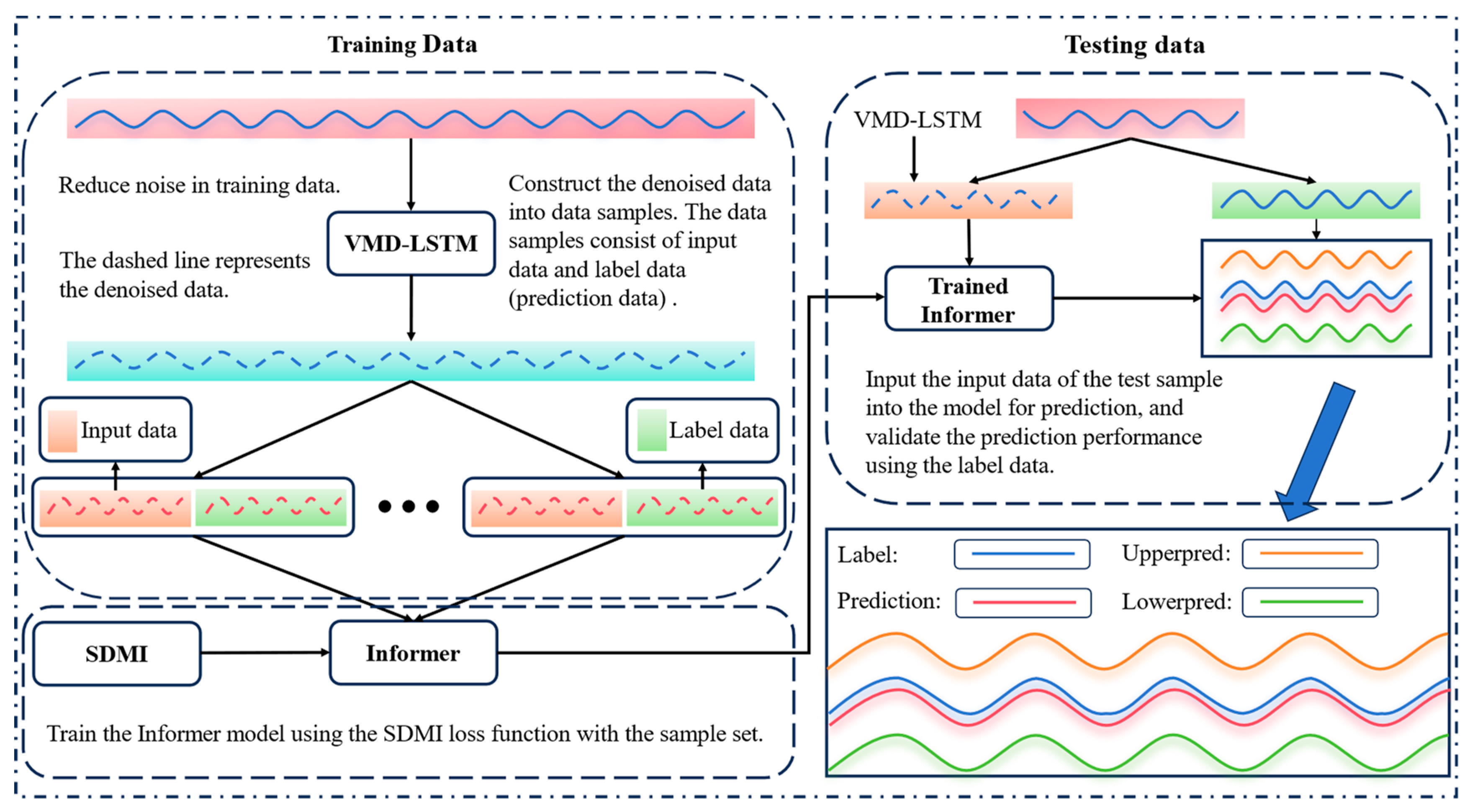
3. Methodology
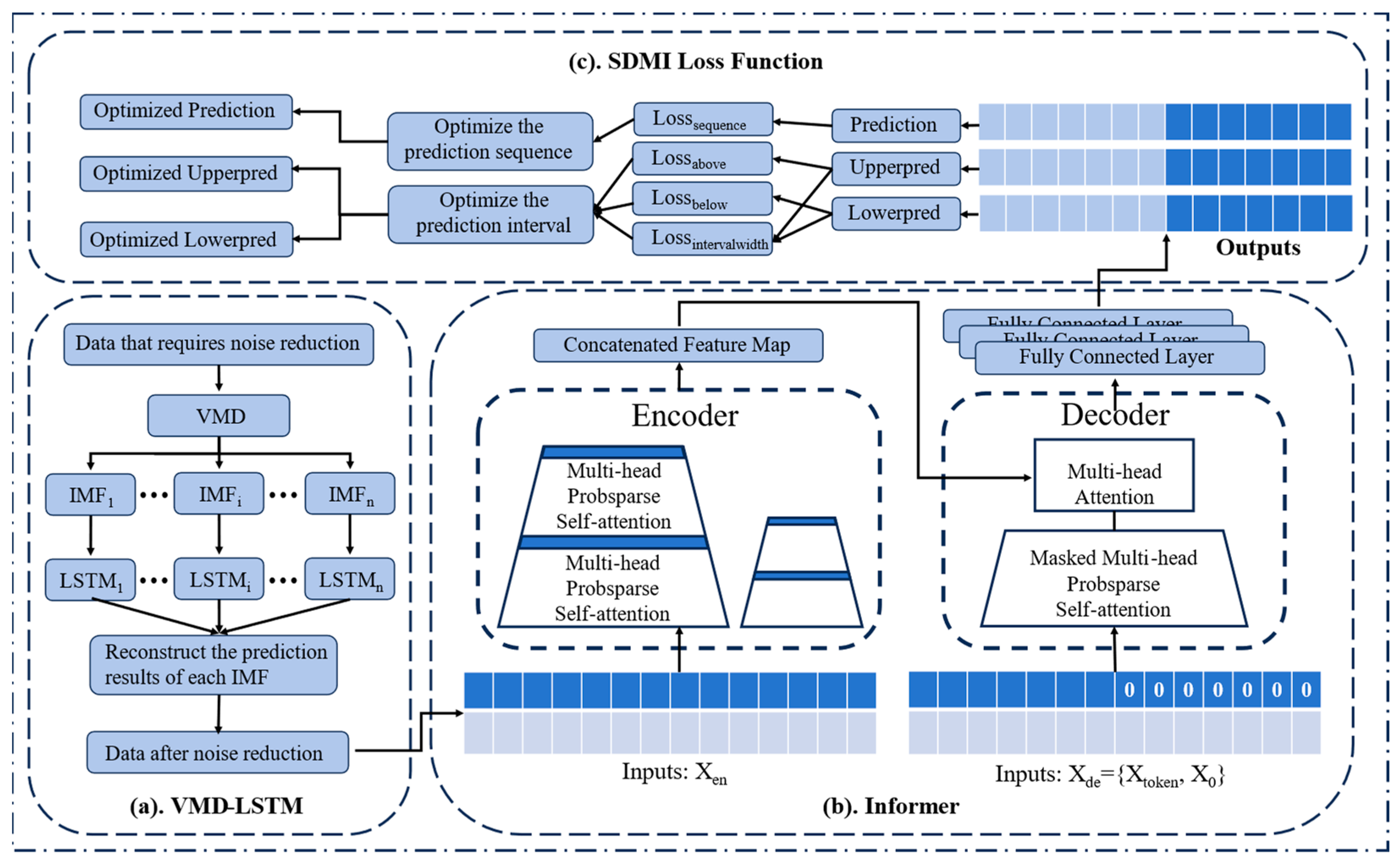
Figure 1 is the schematic diagram of the method proposed. Part a is the data noise reduction part, which is used to remove the noise in the original data, improve the quality of the data, and help to improve the prediction effect of the model. The b part is the Informer prediction model. In order to call the proposed loss function, we modify the output part of the traditional Informer and add two additional fully connected layers to it so that it can output three sequences at the same time. The c part is the process of optimizing the three outputs of the prediction model by the SDMI loss function.
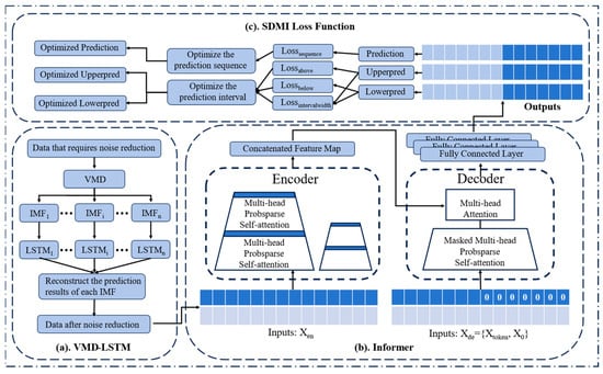
Figure 1.
Schematic diagram of the method proposed.
The rest of this section will explain the proposed data noise reduction method and loss function in detail.
3.1. VMD-LSTM
Considering that the LSTM model has the ability to deal with the long-term dependence of time series data, a combination of VMD and LSTM is used for data denoising. Assuming that the original signal is f, the VMD algorithm decomposes it into K IMF components uk(t), and each component has its own center frequency ωk. The objective of VMD is to minimize the sum of the estimated bandwidths of all IMF components, and the sum of all IMF components is equal to the original signal. This can be achieved by solving the following variational problems:
where K is the number of modes to be decomposed, is the Dirac distribution function, is the partial derivative of time t, and j is the imaginary unit.
To solve the aforementioned constrained variational problem, the VMD algorithm transforms it into an unconstrained problem by introducing a quadratic penalty term α and a Lagrange multiplier λ. The augmented Lagrange expression can be represented as:
Then, the IMF component uk(t) and its center frequency ωk and the Lagrange multiplier λ are iteratively updated by the ADMM algorithm until the termination condition is satisfied.
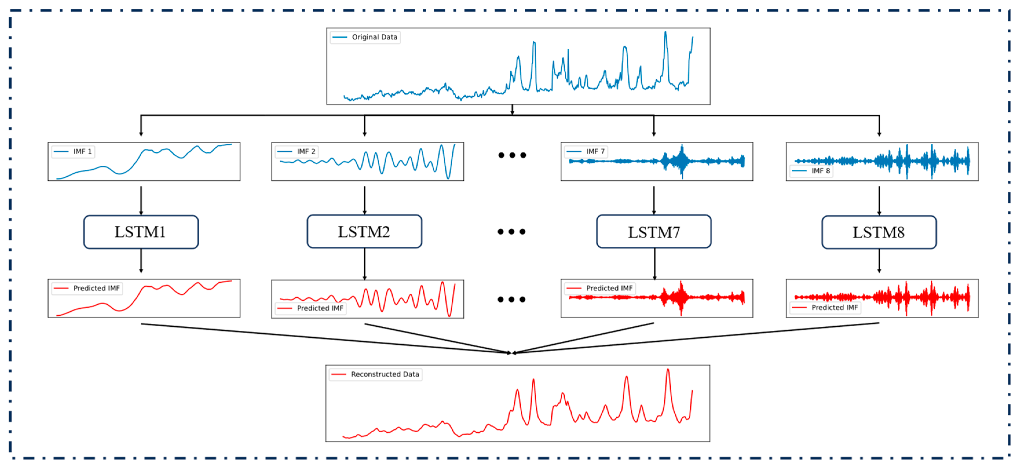
The process of using VMD-LSTM for noise reduction is shown in Figure 2. The original data are decomposed into multiple IMFs, which are then input into the LSTM prediction model for forecasting. Finally, the predicted IMF is reconstructed, and all IMFs can be utilized for reconstruction, or alternatively, only the significant IMFs can be selected for this purpose, yielding the denoised data.
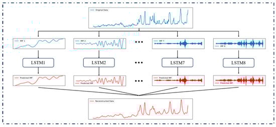
Figure 2.
The process of noise reduction using VMD-LSTM.
By adjusting the parameters of the VMD algorithm or the parameters of the LSTM, the degree of noise reduction can be flexibly adjusted, and the noise reduction process is rapid. Since the purpose of this method is only to reduce noise, although the prediction model is used, it does not need to divide the training set and the test set and directly uses all the data that needs to be denoised for training and prediction. To ensure the effectiveness of noise reduction, the model only needs to predict the data for the next time point. Considering that there is no way to denoise the data that need to be predicted, the label data of the test set should not be denoised.
3.2. SDMI Loss Function
The SDMI loss function consists of two components: the prediction sequence loss and the prediction interval loss. The prediction sequence loss component is composed of the Soft-DTW and MSE loss functions, while the prediction interval loss component comprises a loss function that controls the coverage of the true data by the prediction interval and another loss function that calculates the width of the interval.
3.2.1. Part on Sequence Prediction
The sequence prediction part is used to calculate the error between the predicted sequence and the real value, which is constructed by the Soft-DTW loss function and MSE loss function.
The DTW algorithm is an algorithm used to measure the similarity between two time series. The steps of the DTW algorithm are to first calculate the distance between the points of two time series x and y with length n (Euclidean distance is used in this paper) to form a distance matrix. Then, find a minimum path from (x1, y1) to (xn, yn) in the distance matrix (the sum of elements on the path is the smallest). In order to find out this minimum path, there is the following recursive formula:
where D is the distance matrix, and R(i,j) represents the sum of elements along the minimum path from the starting point (x1, y1) to (xi, yj) in the matrix.
According to the recursive formula, the final R(n,n) is the sum of the elements on the minimum path from (x1, y1) to (xn, yn); that is, the DTW error between the time series x and y. However, the DTW algorithm is discrete and non-differentiable and cannot be used as a loss function of the neural network algorithm. Therefore, the Soft-DTW algorithm turns the DTW algorithm into a continuous and differentiable loss function, mainly by changing the above discrete recursive formula to the following continuous form:
where D is the distance matrix, R(i,j) is the sum of the elements on the minimum path from the matrix (x1, y1) to (xi, yj), and γ is the smoothing parameter to control the degree of softening. The larger the value of γ, the more obvious the softening effect, allowing more flexible alignment; the smaller the value of γ, the weaker the softening effect, and the closer to the traditional DTW.
Therefore, for two sequences x and y with length n, the loss of Soft-DTW is as follows:
Although the Soft-DTW algorithm can calculate the similarity between two time series and is continuously differentiable, making it suitable as a loss function, it does not address the potential time delay issue inherent in the DTW algorithm. To tackle this problem, this paper combines the MSE loss function with Soft-DTW. By leveraging the point-to-point loss calculation method of the MSE loss function, the paper aims to alleviate the time delay issue associated with the Soft-DTW loss function. The formula for MSE is as follows:
where represents the true value of sample i, and represents its corresponding predicted value.
In actual testing, the loss values of the Soft-DTW algorithm and the MSE algorithm may differ significantly. In order to balance the size of these two losses and prevent the model from being biased towards optimizing the loss of one of them, the method of adding 1 to the two losses and then taking the logarithm is adopted. Therefore, the loss function for the sequence prediction part is as follows:
where is the weight of controlling Soft-DTW loss and MSE loss.
3.2.2. Part on Interval Prediction
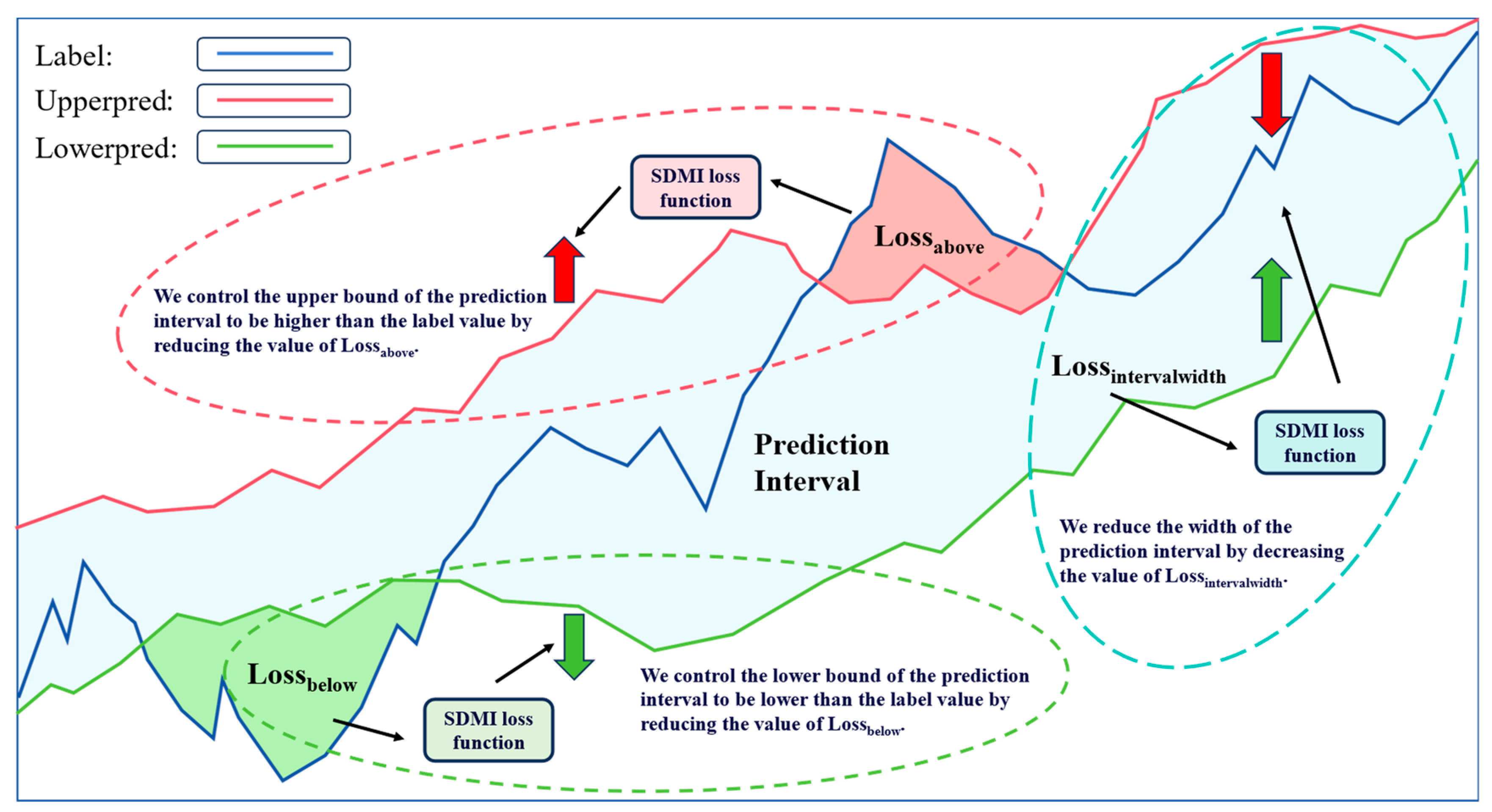
In this part, the loss function for optimizing the prediction interval is designed to ensure that the interval contains the true value as much as possible while keeping the width of the interval as narrow as possible. This method is characterized by its ease of implementation and computation, strong scalability, and wide applicability.
Figure 3 is a schematic diagram of interval prediction, where Label represents the true value (or label) sequence, Upperpred represents the upper bound of the prediction interval, and Lowerpred represents the lower bound of the prediction interval.
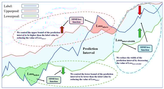
Figure 3.
Schematic diagram of interval prediction.
The prediction interval partially accepts sequences for its upper and lower bounds. It is hoped that the true values can be contained within the prediction interval as much as possible. To achieve this, we only calculate the loss for true values that are higher than the upper bound or lower than the lower bound of the prediction interval. The errors between the true values within the prediction interval and the upper/lower bounds are recorded as zero. Therefore, the sum of the loss functions for the upper and lower bounds constitutes the loss function that controls the coverage of the prediction interval, as shown in the following formula:
where n is the length of the sequence (i.e., the number of data points included), lowerpredi is the i-th value of the lower bound of the prediction interval, upperpredi is the i-th value of the upper bound of the prediction interval, and labelsi is the i-th value of the true value sequence.
In order to prevent the distance between the upper and lower bounds of the prediction interval from being too large, which makes the uncertainty prediction meaningless, the formula used to control the distance between the upper and lower bounds is as follows:
The prediction interval requires adjusting the weights of both interval coverage and interval width based on the prediction results. When the interval is too wide, the weight of the loss function for interval width should be increased. Conversely, when the interval fails to encompass the majority of true data points, the weight of the loss function for interval coverage needs to be raised. To achieve this, two weight parameters are necessary for combination. Thus, the loss function for the prediction interval can be expressed as follows:
where and are weight parameters.
By combining the interval prediction loss with the sequence prediction loss, minimizing the overall loss can simultaneously optimize the model’s outputs of the predicted sequence and the upper and lower bounds of the prediction interval. The loss function, named SDMI, is formulated as follows:
The SDMI loss function should not merely focus on minimizing the loss; it also requires adjusting the sizes of the three weight parameters based on the actual prediction scenario to achieve optimal prediction results.
In order to use the SDMI loss function proposed, it is necessary to add two fully connected layers to the output part of the prediction model. These layers are used to generate the upper and lower bounds of the uncertainty interval, which are then optimized together with the predicted sequence.
4. Experiments
4.1. Data Description
The data used comes from time series data collected from 24 oil wells of an oilfield company in China, numbered sequentially from Well 1 to Well 24. The data covers a time span from June 2016 to March 2022. After unifying the sampling interval of these data to 30 min and excluding features with high null value rates, a total of 970,234 data entries were collected, including 56 characteristics such as temperature and pressure.
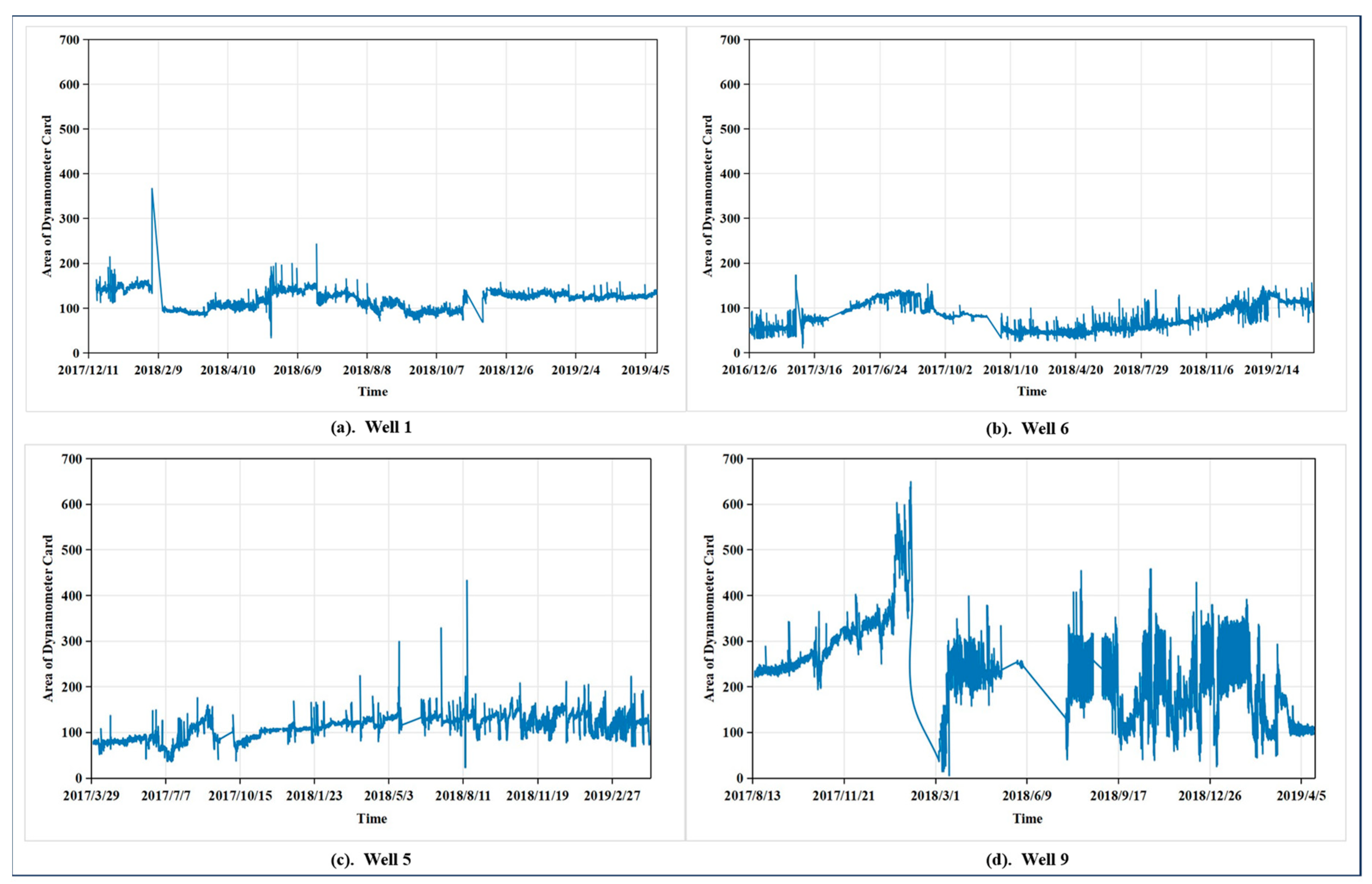
An oil well dynamometer card is a closed curve graph composed of the relationship between load and displacement, used for analyzing the working condition of the pumping unit and diagnosing downhole faults. On the dynamometer card, the horizontal axis represents the distance moved by the polished rod (in meters), and the vertical axis represents the load on the polished rod (in kilonewtons). The enclosed area can be measured in kilonewton-meters (kN·m). Figure 4 shows the area data of dynamometer cards for four different oil wells, data that are crucial for identifying faults in oil wells. The instantaneous peaks in the figure reflect the malfunction of oil wells caused by wax deposition. In subgraph d, there is a sharp decline in the data, dropping rapidly from 650 to nearly 0. This change is due to the missing records from 3 February 2018, to 4 March 2018, in the dataset. Figure 4 presents the raw data after smoothing processing, and to ensure temporal continuity, the missing data for the omitted period were automatically filled in when plotting the graph. However, in the process of constructing the sample set for this study, we strictly selected continuous data sequences for each sample. Therefore, for time periods with large-scale data missing, such as this one, we did not include them in the analysis. The figure indicates that the oil well data do not exhibit obvious seasonal or cyclical characteristics, and the data show relatively intense fluctuations along with significant noise. Clearly, it is quite challenging to accurately predict data changes over a longer future period for such data, which is why we focus on forecasting the data’s trend rather than merely emphasizing the fit between the predicted and actual data. Furthermore, the data sampling interval in this paper is set at half an hour to verify the effectiveness of the proposed prediction method under conditions of intense data fluctuation. In practice, if conditions permit, a longer time interval can be adopted. This not only extends the period for which future data changes can be predicted when forecasting the same number of time points but also reduces the degree of data fluctuation, thereby enhancing prediction performance.
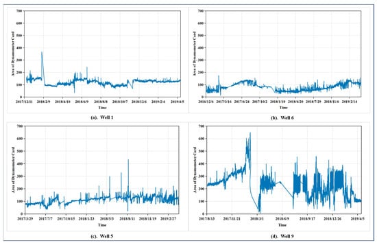
Figure 4.
Time series data of four oil wells. (a) Well 1, (b) Well 6, (c) Well 5, (d) Well 9.
Historical time series data from oil wells are utilized to predict the next 48 data points. Given that the data sampling interval is half an hour, it is equivalent to predicting one day’s data. However, as the sampling interval changes, the length of predictable time will adjust accordingly. For instance, if the sampling interval is set to one day, it would be equivalent to forecasting data for the next 48 days. Regarding the number of input features, SHAP value analysis is employed to select features relevant to the prediction target. Only strongly correlated features, along with the target feature itself, are chosen as input features for the model. Consequently, the number of input features is not fixed.
4.2. Normalization
The data are normalized using linear normalization (min–max) to map the original data to the range of [0,1]. The formula is:
where min(x) represents the minimum value in the original data, max(x) represents the maximum value in the original data, x represents the data that needs to be normalized, and x’ represents the normalized data.
4.3. Experimental Details
4.3.1. Evaluation Metrics
This paper mainly uses the visualized prediction results as the evaluation metric. However, in order to provide a more comprehensive evaluation, the R-squared value is employed to assess the error between the predicted sequence and the actual sequence. The formula for R-squared is as follows:
where represents the true value, represents the predicted value, is the sample mean, is the error between the predicted value and the true value, and is the error generated between the true value and the mean.
4.3.2. Parameter Setting
The three weight parameters of the SDMI loss function proposed need to be adjusted according to the specific dataset. The value of can be determined based on the comparison between the predicted sequence and the true sequence. If the predicted sequence exhibits significant time delay, should be decreased to increase the proportion of the MSE (Mean Squared Error) loss function. Conversely, if the predicted sequence fails to reflect the trend of the true sequence, should be increased to enhance the proportion of the Soft-DTW (Soft Dynamic Time Warping) loss function. The value of is set according to how well the prediction interval covers the true values; if many true values fall outside the prediction interval, should be increased. The value of is determined by the width of the interval; if the interval is too wide, should be increased. The settings of and influence each other, and multiple adjustments may be needed to achieve the best prediction performance. As for the choice of K, it can be determined by comparing the effects of using different values of K.
In the dataset presented in this paper, the three weight parameters can be approximately set as follows: is 0.5, is 0.03, and is 0.005. For the VMD algorithm, the number of K is 6, alpha is 2000, and tol is 1 × 10⁻⁷. The Adam optimizer is selected with a learning rate of 0.0005. The relevant parameters and iteration times of the LSTM and Informer models may vary depending on different datasets, and optimization algorithms such as Particle Swarm Optimization and Grey Wolf Optimizer can be used for optimization. In total, 80% of the data are used as the training dataset, while 20% are used as the testing dataset.
4.3.3. Experimental Procedure
The main experimental procedure is shown in Figure 5. The original data are divided into a training set and a test set. The VMD-LSTM algorithm described in Section 3.1 is used to denoise the training data and the input data of the test set for the oil well time series data. The denoised training data are then constructed into a training sample set to train a time series prediction model using SDMI as the loss function. Finally, the input data of the test set are used for prediction, and the prediction results are validated against the label data of the un-denoised test set. Additionally, an LSTM model is constructed for comparison.
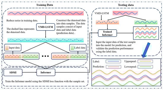
Figure 5.
Flowchart of experimental procedure.
5. Results and Discussion
The prediction results presented in the text are those obtained on the test set, meaning they were generated from data that the model had not previously seen. This process simulates predicting future unknown data, allowing for an assessment of the model’s ability to forecast future data. In this section, we will present the experimental results of our proposed method from three aspects: loss function, data denoising, and uncertainty prediction intervals.
5.1. Comparison of Loss Functions and Models
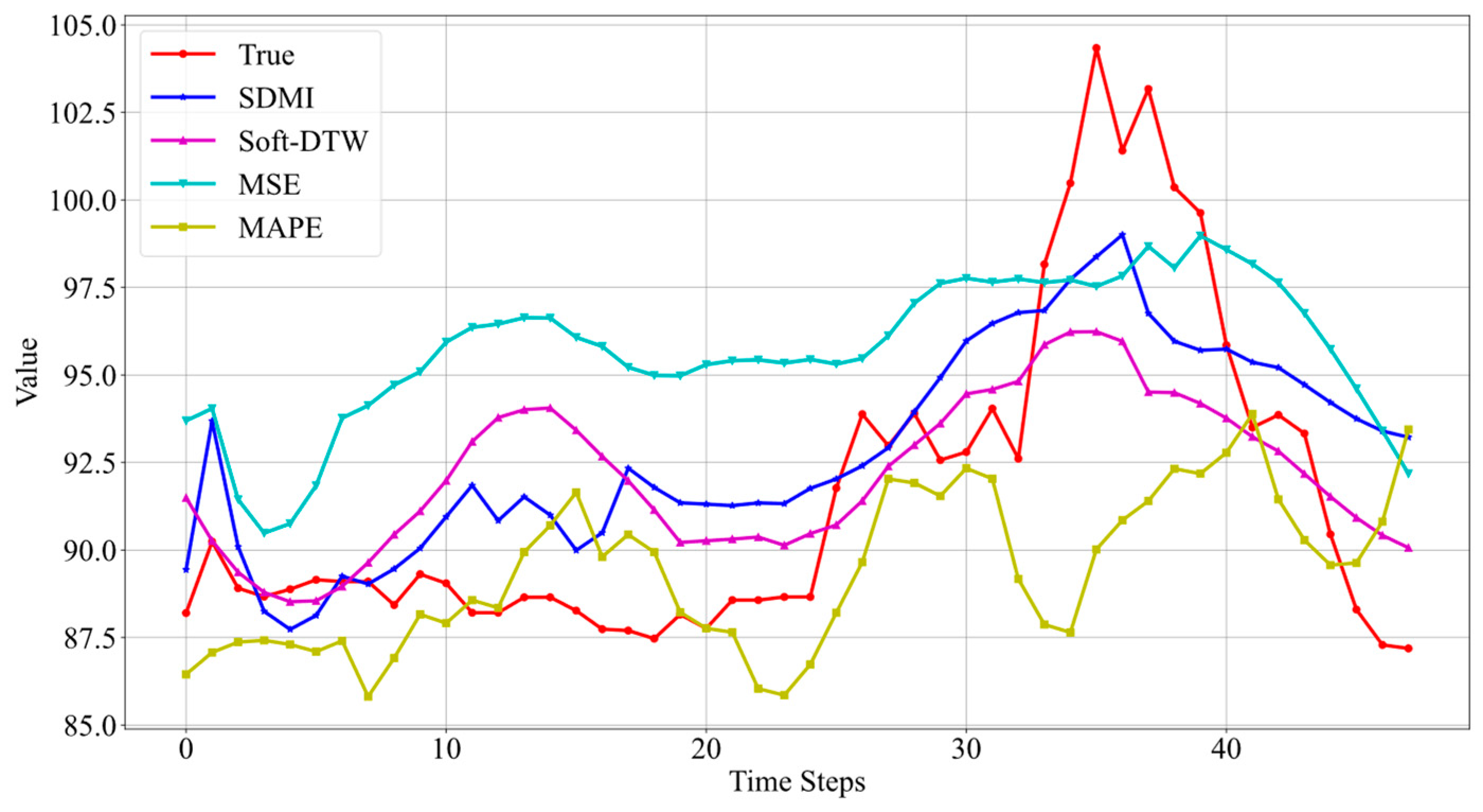
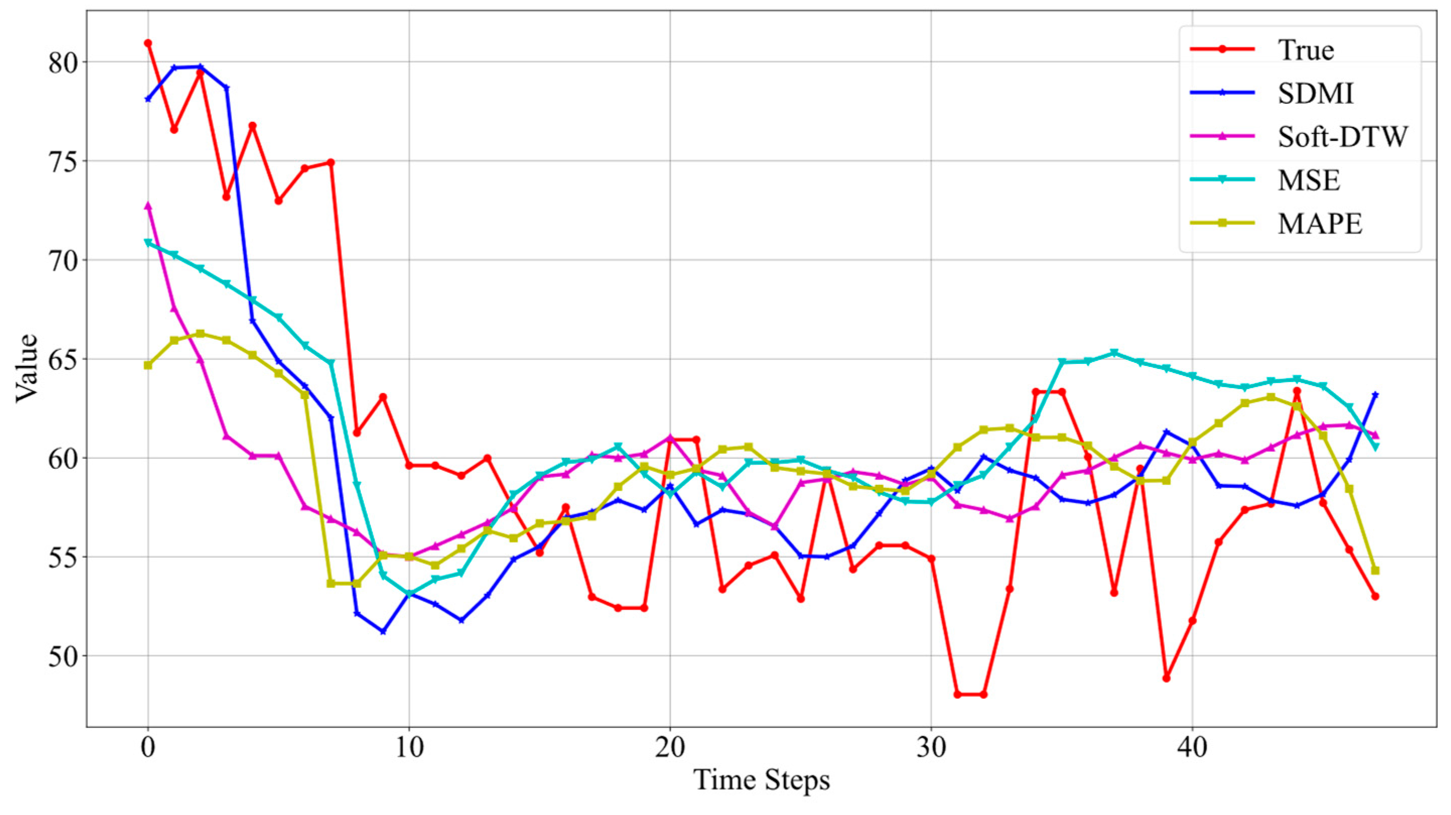
The LSTM model and the Informer model are trained separately on data from three different oil wells using four loss functions: SDMI, Soft-DTW, MSE, and MAPE. The prediction results are visualized, with the prediction results for Well 3 shown in Figure 6 and Figure 7. As we focus here on the sequence prediction part using the SDMI loss function, the prediction interval part is not visualized, and a higher weight is assigned to the sequence prediction component in the SDMI loss function.
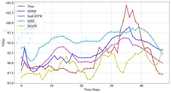
Figure 6.
Prediction results of LSTM models using different loss functions.
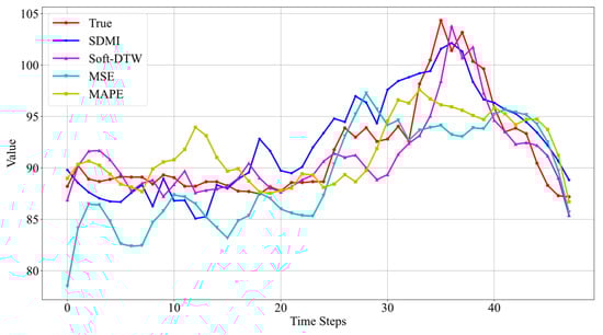
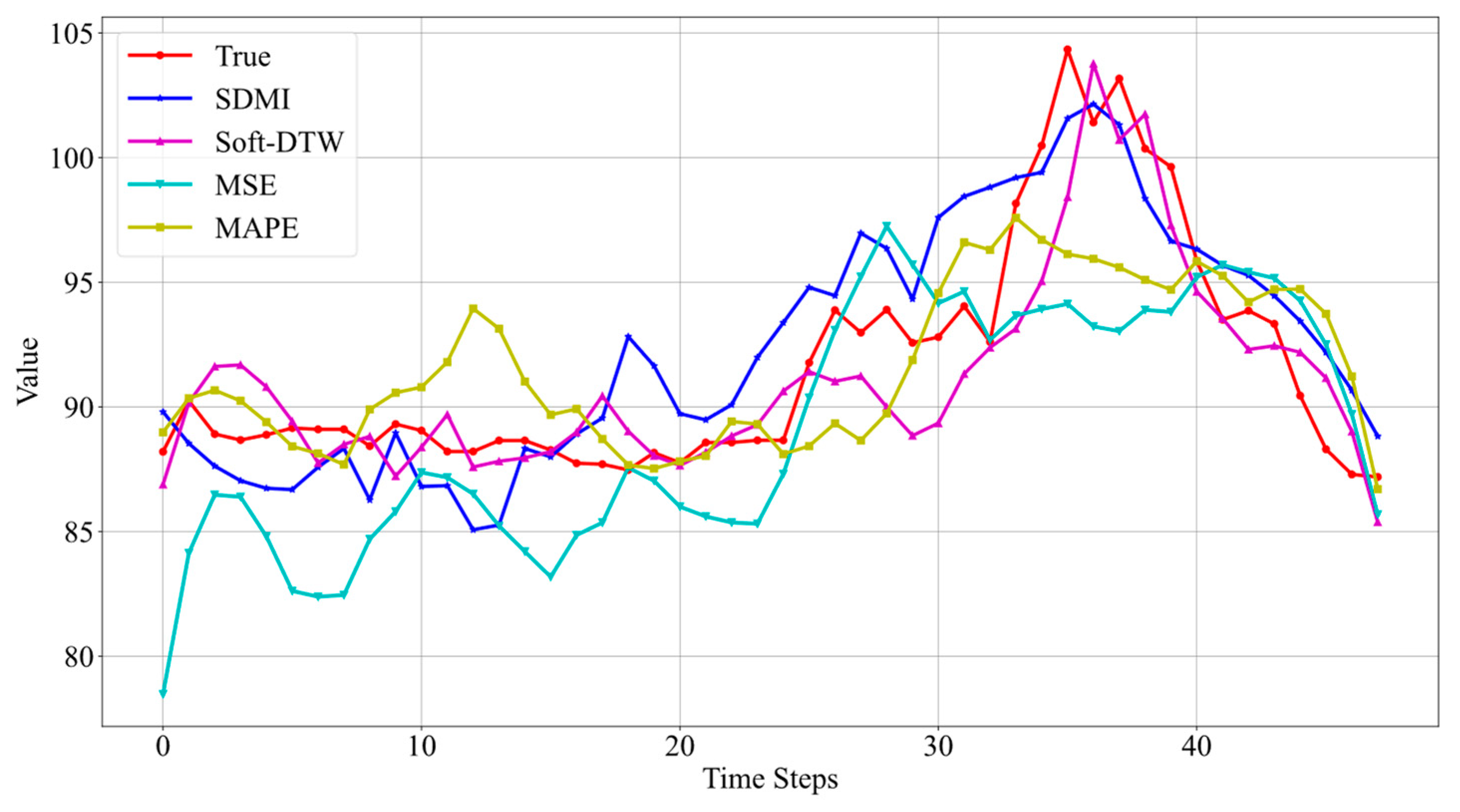
Figure 7.
Prediction results of Informer models using different loss functions.
From the prediction results in Figure 6, it can be seen that when using SDMI as the loss function, the prediction effect of the LSTM model is the best. Although it does not fit the real data perfectly, it can reflect the trend of the real data. The other three loss functions do not perform as well.
The prediction results from Figure 7 indicate that the Informer model outperforms LSTM, particularly when using SDMI and Soft-DTW as loss functions. Both accurately reflect the trend of real data changes. However, when using Soft-DTW, the predicted results start to rise at the 30th data point, whereas the real data starts to rise at the 24th data point, indicating a certain time delay. The results using SDMI start to rise from the 22nd data point, and those using MSE start from the 23rd. This shows that the SDMI loss function, which combines MSE and Soft-DTW, does indeed address the time delay issue associated with Soft-DTW to a certain extent. Furthermore, the results using MSE alone fail to predict the data’s rise to a peak followed by a decline, but when combined with Soft-DTW, the trend is correctly predicted. This further demonstrates the advantages of combining these two loss functions.
The above results indicate that the Informer model exhibits better prediction performance than the LSTM model, suggesting that the Informer model has superior capabilities in long time series prediction tasks. This may be attributed to innovations in the Informer model, such as its ProbSpars self-attention mechanism. Due to space constraints, only the prediction results of the Informer model are shown for the remaining two datasets, and the specific R-squared comparisons between the two models are presented in Table 1.

Table 1.
R-squared values of prediction results for two models using different loss functions on three datasets.
From the figures and table, it can be observed that the model trained using the SDMI loss function achieves the best prediction performance and can accurately forecast future trends in the data.
The prediction results of the Informer model using different loss functions on the other two datasets are shown in Figure 8 and Figure 9.
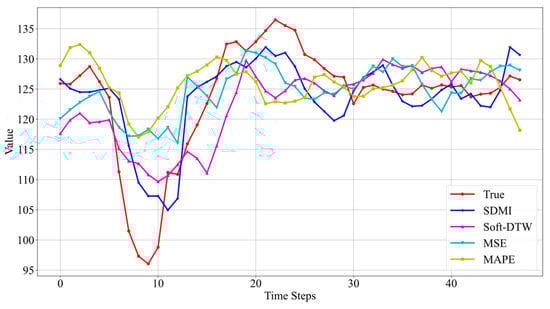
Figure 8.
Prediction results on Well 5.
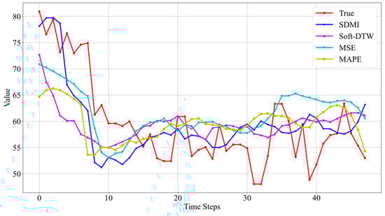
Figure 9.
Prediction results on Well 8.
From the results in Figure 8, it can be seen that the best prediction performance is still achieved when using SDMI as the loss function. Although there is a certain gap between the predicted minimum value and the actual minimum value of the sequence, the model successfully predicts the trend of the data. Furthermore, compared to Soft-DTW, the addition of MSE improves the issue of certain time delays, once again validating the effectiveness of the method proposed.
Figure 9 shows that there are significant fluctuations in the real sequence in the latter half, and the prediction model fails to predict these fluctuations when using all loss functions. This indicates the difficulty in predicting long time series with substantial fluctuations, which is a common challenge in long time series prediction. Nevertheless, despite the less accurate predictions in the latter half, when using SDMI as the loss function, the general trend of the data changes can still be predicted.
This demonstrates that, compared to existing loss functions, the SDMI loss function proposed achieves better results in long time series prediction tasks. This is because the SDMI loss function proposed in this paper combines the advantages of both Soft-DTW and MSE. Soft-DTW is better at calculating the similarity in shape and trend between two time series, making it more suitable for long-term time series prediction compared to traditional loss functions. On the other hand, MSE focuses more on the accuracy of point-to-point predictions, effectively addressing the time delay issue present in Soft-DTW. By combining the two, the overall accuracy of the predicted sequence can be improved.
The results from Table 1 indicate that the predictive performance of the Informer model is higher than that of LSTM. This is consistent with the findings in the literature [35] that the prediction performance of the Informer model is better than that of LSTM. Therefore, only the Informer model will be used for predictions in the remainder of this paper.
5.2. Efficacy of Data Denoising
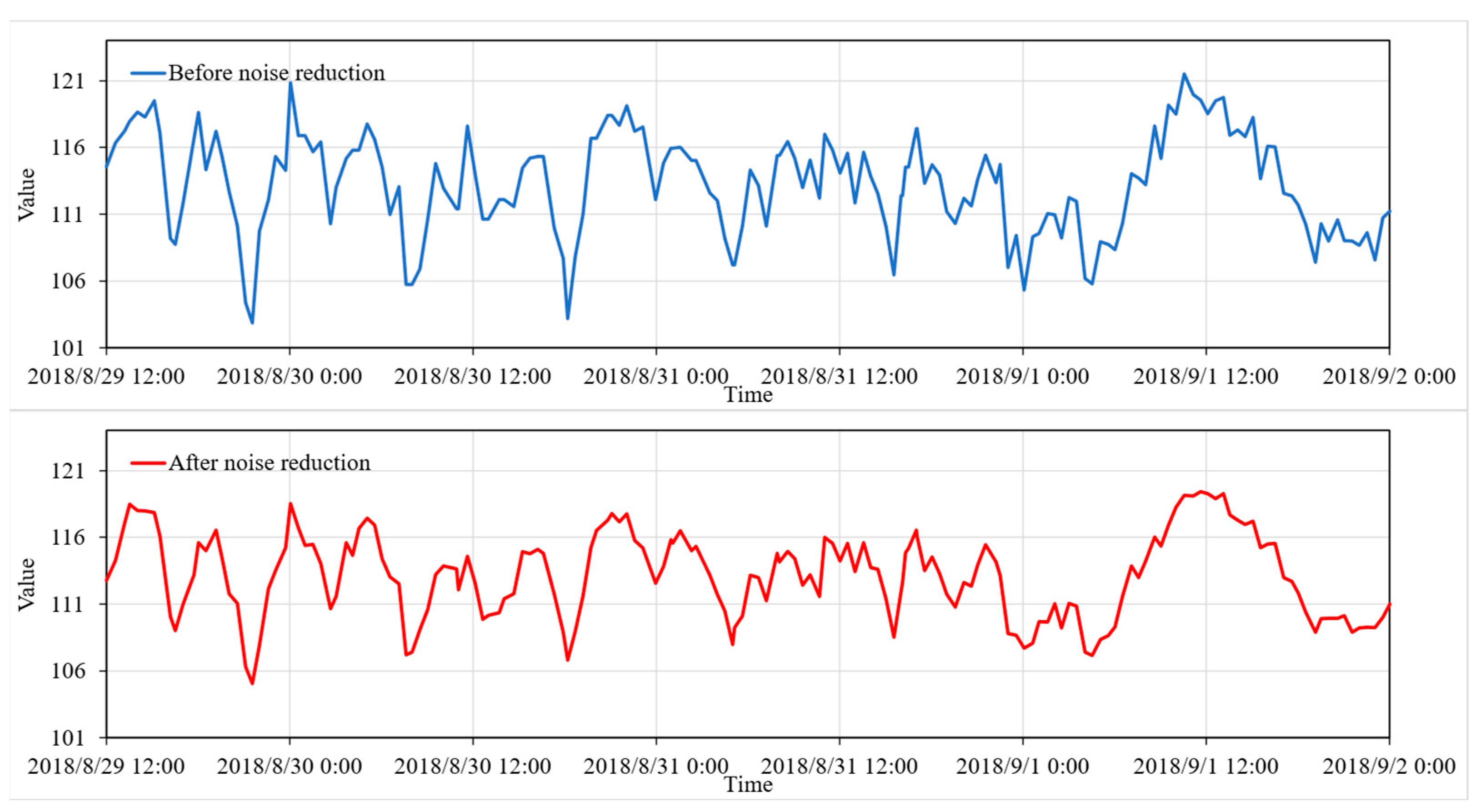
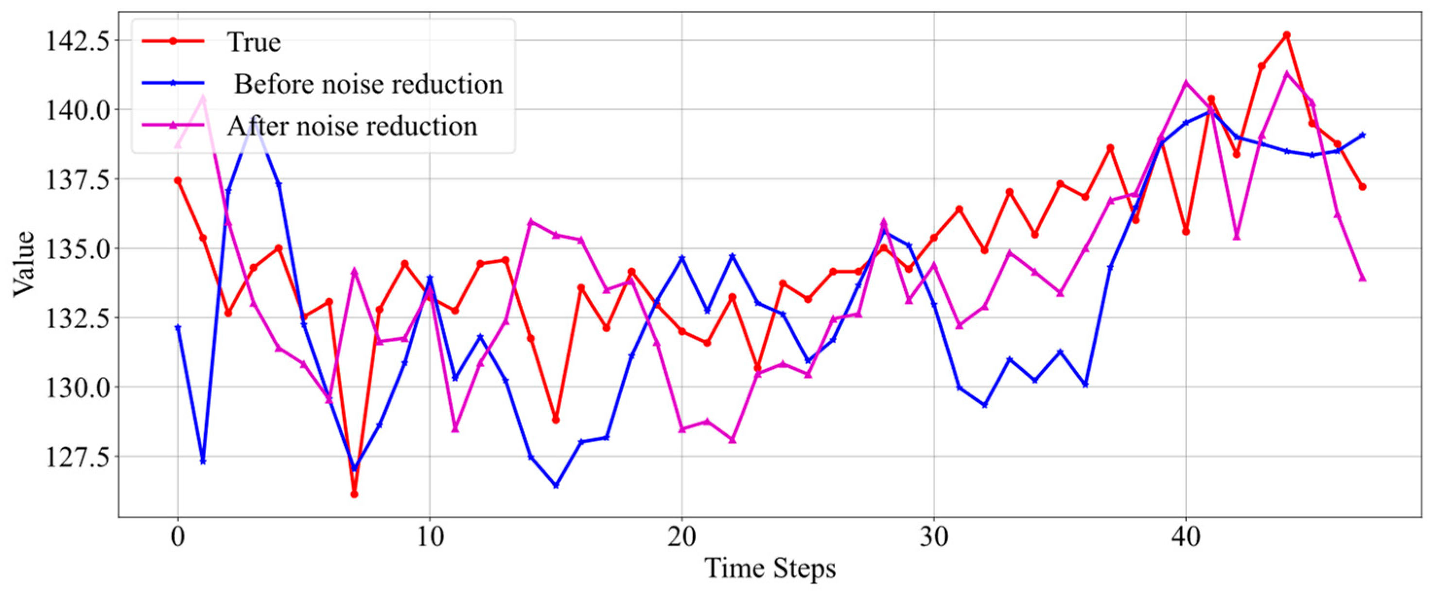
Based on the prediction results from Figure 9 in Section 5.1, it can be seen that dramatic data fluctuations are difficult to predict. Similarly, using data with intense fluctuations to train the model will also affect the effectiveness of model training. Therefore, in many cases, it is necessary to preprocess the training data by denoising it to eliminate noise and smooth the data before training the model. Considering that the data to be predicted should be unknown and cannot be denoised, this paper does not apply denoising to the label data of the test set. Furthermore, taking into account that outliers in oil well data sometimes contain important information, excessive denoising is not performed on the data. The denoising method employed is the VMD-LSTM denoising approach described in Section 3.1. A comparison of the data before and after denoising is shown in Figure 10.

Figure 10.
Comparison before and after data noise reduction.
It can be seen that the denoised data retains all the information regarding the trends of the real data while making the data smoother. By adjusting the parameters of the VMD-LSTM, the degree of data denoising can be controlled as needed.
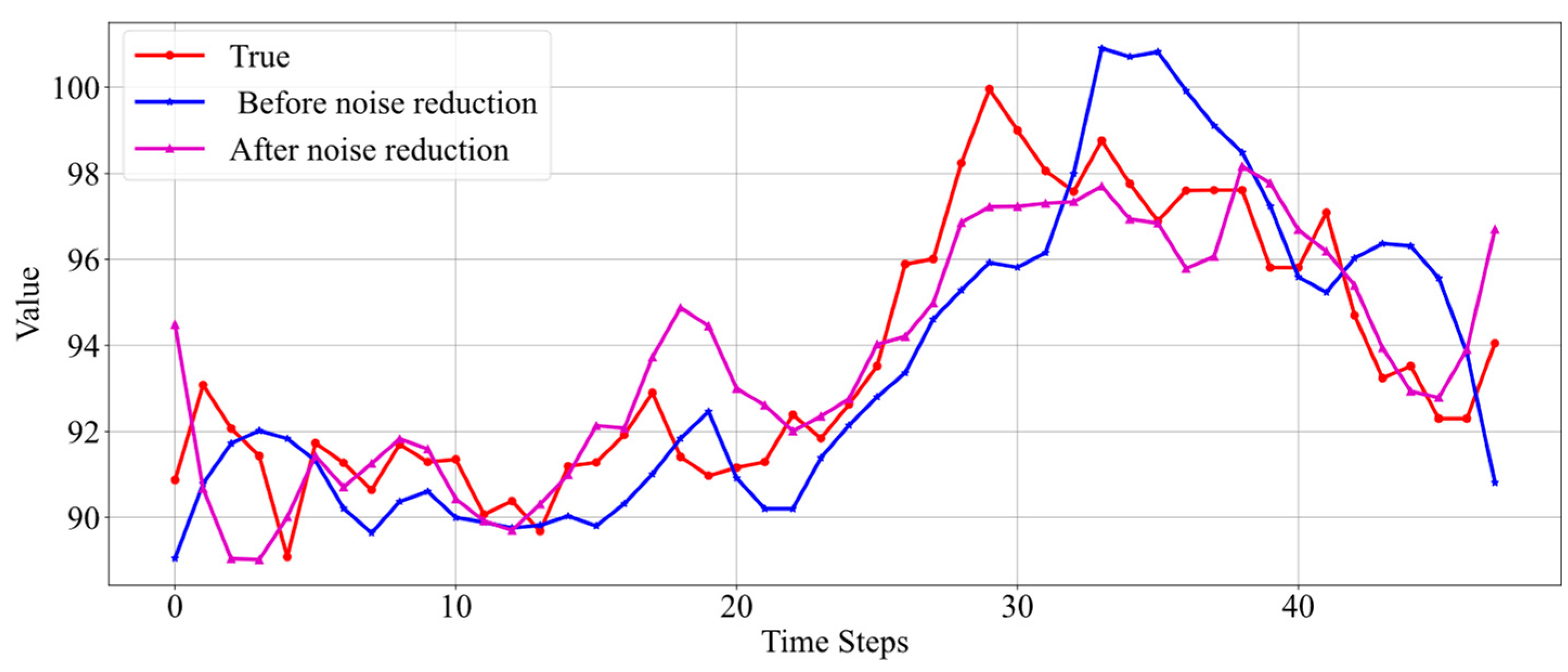
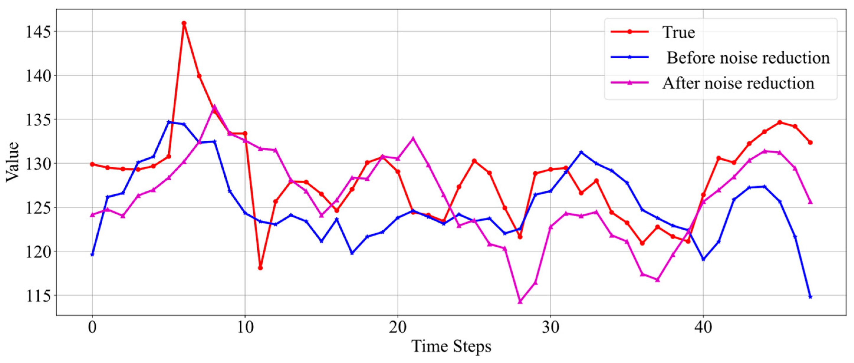
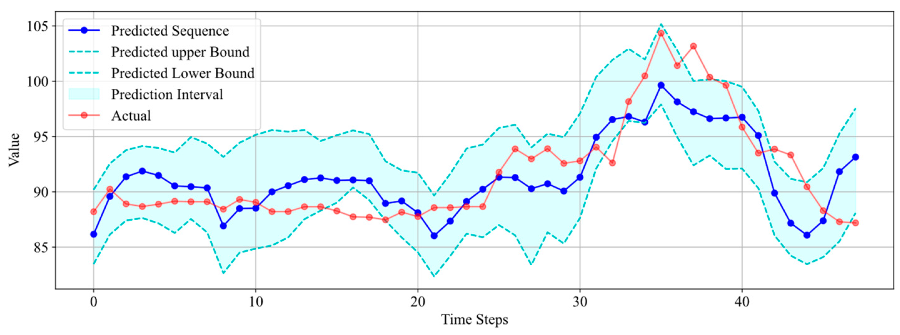
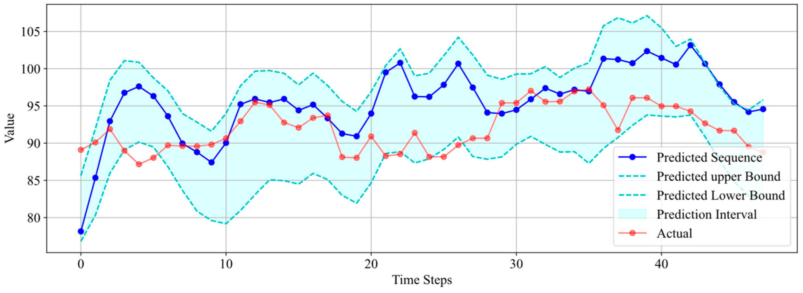
To compare the prediction performance before and after data denoising, the following approach is applied to data from three wells. First, the oil well data are denoised, and an Informer model is trained and used for prediction; then, an Informer model with identical parameters is trained using the original non-denoised real data and used for prediction. Subsequently, the prediction results obtained using denoised data are compared with those obtained using real data, as shown in Figure 11, Figure 12 and Figure 13.
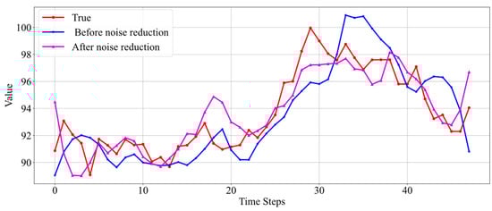
Figure 11.
Comparison of prediction results before and after data noise reduction for Well 4.
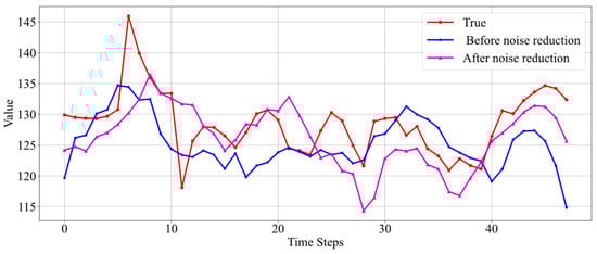
Figure 12.
Comparison of prediction results before and after data noise reduction for Well 7.

Figure 13.
Comparison of prediction results before and after data noise reduction for Well 5.
The results in Figure 11 show that when the real data themselves are relatively stable and there are no drastic fluctuations, both the model trained on denoised data and the model trained on real data yield good prediction results, accurately reflecting the data’s trend. There is not a significant difference in prediction performance, but overall, the prediction results from the denoised data are slightly better and more stable.
Unlike Figure 11, the real data in Figure 12 exhibit significant fluctuations. Neither the prediction results before noise reduction nor those after accurately reflect the data’s trend. However, the prediction results based on noise-reduced data are still better. Figure 13 also presents a case where real data fluctuate greatly. According to the results shown in the figure, the predictions made by the model trained without noise-reduced data also exhibit considerable fluctuations and do not effectively capture the trend of the real data changes. Conversely, the model trained with noise-reduced data yields predictions with smaller fluctuations and accurately reflects the trend of the real data.
From the above results, it can be seen that the prediction results of the model trained with noise-reduced data better reflect the trend of real data changes and are more stable compared to the prediction results of the model trained with the original real data. The comparison of R-squared values and SDMI loss size for the prediction results before and after data noise reduction for the three wells is presented in Table 2.
Table 2.
Comparison of prediction results before and after data noise reduction.
From the results presented in Table 2, it can be observed that utilizing noise-reduced data for model training enhances the model’s predictive performance. Additionally, it is noted that the R-squared values for Well 7 and Well 5 are relatively low. This is because the real data used for validating the prediction results have not been noise-reduced. Therefore, in situations where the real data exhibit significant fluctuations, the R-squared values of the prediction results will not be too high. However, for long-term time series prediction, we are more concerned with the trend of data changes, and the degree of fitting between the prediction results and the real data is not as crucial.
5.3. Uncertainty Prediction Interval
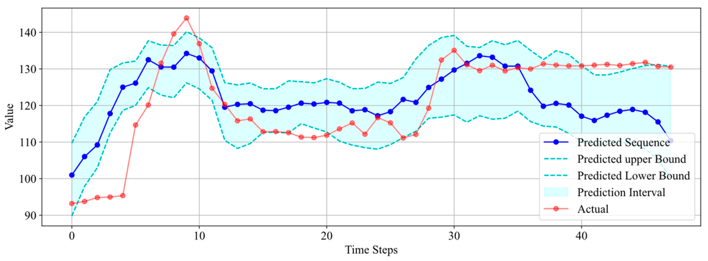
The Informer model was trained using noise-reduced training data and SDMI was employed as the loss function, subsequently performing uncertainty interval prediction on the test data. In this section, we not only focus on the accuracy of the predicted sequences but also on the accuracy of the prediction intervals. During model training, it is necessary to adjust the three weight parameters of the SDMI loss function based on the prediction results of the trained model. This adjustment balances the degree of optimization between the predicted sequences and prediction intervals, aiming to achieve the best prediction performance. Below, prediction results from several oil well datasets have been selected for analysis.
The results from Figure 14 indicate that both the predicted sequence and interval accurately reflect the trend of the real data changes. The predicted uncertainty interval encompasses a majority of the real data points, with only six data points falling outside the predicted interval. Furthermore, the width of the interval is controlled within 10, ensuring the effectiveness of the uncertainty prediction.

Figure 14.
Interval prediction results for Well 3.
The results in Figure 15 indicate that the predicted sequence does not accurately reflect the trend changes in the real sequence. However, the predicted uncertainty interval still encompasses a majority of the real data points, with only seven data points falling outside the interval, demonstrating that the predicted uncertainty interval remains effective. This also reflects the robustness of this method, because it is sometimes the case that the predicted sequence deviates from the true values. It is precisely in such situations that an uncertainty interval is needed to contain the real data, thereby avoiding erroneous judgments caused by inaccurate predictions.

Figure 15.
Interval prediction results for Well 5.
Figure 16 shows that the real data initially experienced a dramatic change, rising from 93.21 to 143.91 in a short period. Although the predicted results did not fit the real data perfectly, except for the discrepancy between the predicted trend and the actual trend starting from the 36th data point, the rest of the predictions were still able to capture the trend of the real data. Even though the trend was not accurately predicted from the 36th data point onwards, the upper bound of the prediction interval was close to the last 12 data points, indicating that the uncertain prediction still had some validity.
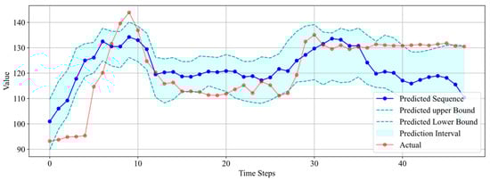
Figure 16.
Interval prediction results for Well 8.
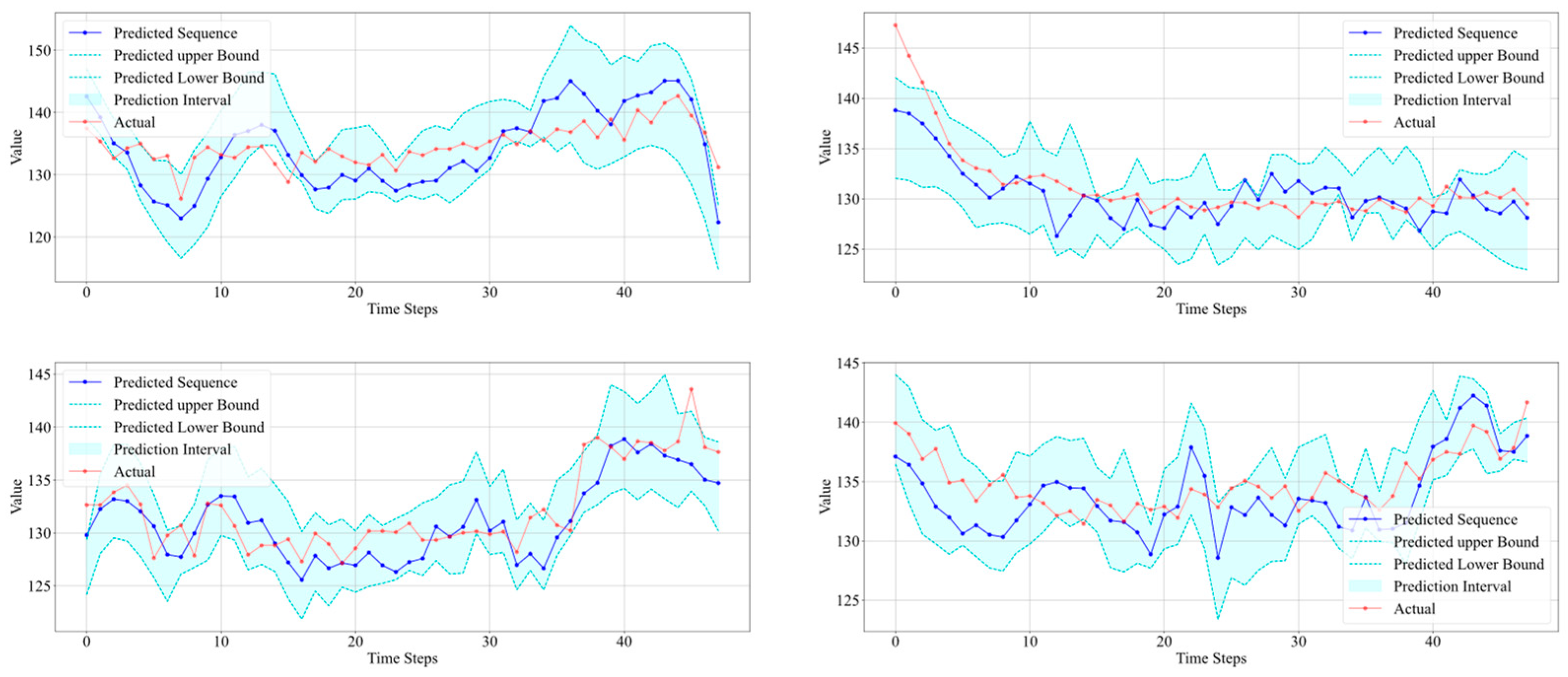
The prediction results on four additional datasets are also plotted, as shown in Figure 17.
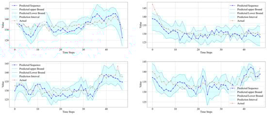
Figure 17.
Interval prediction results for four wells.
Table 3 provides detailed information on the interval prediction results based on data from seven wells.
Table 3.
Prediction interval results on data from seven wells.
From Table 3, it can be noticed that the R-squared values for Well 5 and Well 8 are negative. However, this does not necessarily indicate poor prediction results. As can be seen from Figure 15 (Well 5), while the predicted sequence does not closely match the actual data, it roughly reflects the trend of the real data. Importantly, the prediction interval covers 84% of the actual data quite well, and the interval width is not excessively high. As a result of uncertainty prediction, this is acceptable. As for Figure 16 (Well 8), the predicted sequence actually reflects the trend of the real data very well. It is only due to the dramatic fluctuations in the actual data, with a data span of 50.71, that the R-squared value is low. The prediction results for the other five wells are all very good, meeting the requirements of uncertainty prediction in terms of both interval coverage and interval width. The experimental results above demonstrate that the uncertainty interval prediction method proposed has high accuracy and robustness and can be applied to different datasets.
6. Conclusions
Experimental results confirm that the proposed SDMI loss function outperforms existing loss functions in terms of prediction accuracy. On datasets from Wells 3, 5, and 8, the R-squared values of the prediction results are 0.7319, 0.6988, and 0.4541, respectively, which are better than those obtained using other loss functions. The data after noise reduction can indeed improve the performance of model prediction, especially in the case of severe fluctuation of real data. Compared to the prediction results using the original data, the R-squared values improved by 5.5%, 76.8%, and 0.7% for Wells 4, 7, and 5, respectively. The improvement in prediction performance is more intuitively observable through the visualization of the prediction results. Lastly, the effectiveness of the predicted uncertainty intervals is also validated. Experimental results demonstrate that the average coverage rate of the predicted uncertainty intervals across data from seven wells is 81.4%, with a maximum reach of 90%. The experimental results indicate that the method proposed in this paper outperforms existing methods in the task of oil well monitoring data prediction.
Furthermore, the prediction method proposed in this paper is not only applicable to time series data from oil wells but can also be utilized for time series data prediction tasks across various industries.
In the future, we will continue to study how to design a hyper-parameter optimization method to automatically optimize the three parameters of the SDMI loss function proposed in this paper and how to improve the Soft-DTW algorithm to improve its calculation speed when dealing with long sequences. The data in this paper originate from the same oil field, thus sharing the same physical characteristics, similar types, and utilizing similar equipment. For different oil fields, there may be differences due to factors not considered in the analysis. We will address this issue in future research by studying the generalization capability of the model.
Author Contributions
Conceptualization, Y.S. and Y.X.; Methodology, Y.S. and R.Z.; Validation, Y.S.; Formal analysis, Y.S., Y.X. and W.W.; Investigation, Y.S., W.W. and R.Z.; Data curation, X.W., Y.X. and W.W.; Writing—original draft, Y.S.; Writing—review & editing, X.W.; Visualization, Y.S.; Supervision, X.W., Y.X. and R.Z.; Project administration, X.W.; Funding acquisition, X.W. All authors have read and agreed to the published version of the manuscript.
Funding
This research was funded by the National Natural Science Foundation of China (No. 52204027), the Qing Lan Project of Jiangsu Province (2024), and the Postgraduate Research and Practice Innovation Program of Jiangsu Province (No. KYCX24_3218).
Data Availability Statement
The authors do not have permission to share the data.
Conflicts of Interest
We declare that we have no conflicts of interest in this work. We declare that we have no commercial or associated interests that represent a conflict of interest related to the submitted work.
References
- Lu, H.; Guo, L.; Azimi, M.; Huang, K. Oil and Gas 4.0 era: A systematic review and outlook. Comput. Ind. 2019, 111, 68–90. [Google Scholar] [CrossRef]
- Dasgupta, S.N. Digitalization in petroleum exploration & production: The new game changer. In Innovative Exploration Methods for Minerals, Oil, Gas, and Groundwater for Sustainable Development; Elsevier: Amsterdam, The Netherlands, 2022; pp. 429–439. [Google Scholar] [CrossRef]
- Bist, N.; Panchal, S.; Gupta, R.; Soni, A.; Sircar, A. Digital transformation and trends for tapping connectivity in the Oil and Gas sector. Hybrid Adv. 2024, 6, 100256. [Google Scholar] [CrossRef]
- Huang, N.E.; Shen, Z.; Long, S.R.; Wu, M.C.; Shih, H.H.; Zheng, Q.; Yen, N.-C.; Tung, C.C.; Liu, H.H. The empirical mode decomposition and the Hilbert spectrum for nonlinear and non-stationary time series analysis. Proc. R. Soc. Lond. Ser. A Math. Phys. Eng. Sci. 1998, 454, 903–995. [Google Scholar] [CrossRef]
- Dragomiretskiy, K.; Zosso, D. Variational Mode Decomposition. IEEE Trans. Signal Process. 2014, 62, 531–544. [Google Scholar] [CrossRef]
- Kumar, I.; Tripathi, B.K.; Singh, A. Attention-based LSTM network-assisted time series forecasting models for petroleum production. Eng. Appl. Artif. Intell. 2023, 123, 106440. [Google Scholar] [CrossRef]
- Sagheer, A.; Kotb, M. Time series forecasting of petroleum production using deep LSTM recurrent networks. Neurocomputing 2019, 323, 203–213. [Google Scholar] [CrossRef]
- Wu, H.; Liang, Y.; Gao, X.-Z.; Heng, J.-N. Bionic-inspired oil price prediction: Auditory multi-feature collaboration network. Expert Syst. Appl. 2024, 244, 122971. [Google Scholar] [CrossRef]
- Cheng, W.; Ming, K.; Ullah, M. Oil price volatility prediction using out-of-sample analysis-Prediction efficiency of individual models, combination methods, and machine learning based shrinkage methods. Energy 2024, 300, 131496. [Google Scholar] [CrossRef]
- Liang, X.; Luo, P.; Li, X.; Wang, X.; Shu, L. Crude oil price prediction using deep reinforcement learning. Resour. Policy 2023, 81, 103363. [Google Scholar] [CrossRef]
- Al-Sabaeei, A.M.; Alhussian, H.; Abdulkadir, S.J.; Jagadeesh, A. Prediction of oil and gas pipeline failures through machine learning approaches: A systematic review. Energy Rep. 2023, 10, 1313–1338. [Google Scholar] [CrossRef]
- Guang, Y.; Wang, W.; Song, H.; Mi, H.; Tang, J.; Zhao, Z. Prediction of external corrosion rate for buried oil and gas pipelines: A novel deep learning with DNN and attention mechanism method. Int. J. Press. Vessel. Pip. 2024, 209, 105218. [Google Scholar] [CrossRef]
- Kumari, P.; Wang, Q.; Khan, F.; Kwon, J.S.-I. A unified causation prediction model for aboveground onshore oil and refined product pipeline incidents using artificial neural network. Chemical Engineering Res. Des. 2022, 187, 529–540. [Google Scholar] [CrossRef]
- Wang, J.; Meng, Y.; Han, B.; Liu, Z.; Zhang, L.; Yao, H.; Wu, Z.; Chu, J.; Yang, L.; Zhao, J.; et al. Hydrate blockage in subsea oil/gas flowlines: Prediction, prevention, and remediation. Chem. Eng. J. 2023, 461, 142020. [Google Scholar] [CrossRef]
- Li, X.; Guo, M.; Zhang, R.; Chen, G. A data-driven prediction model for maximum pitting corrosion depth of subsea oil pipelines using SSA-LSTM approach. Ocean Eng. 2022, 261, 112062. [Google Scholar] [CrossRef]
- Zhou, G.; Guo, Z.; Sun, S.; Jin, Q. A CNN-BiGRU-AM neural network for AI applications in shale oil production prediction. Appl. Energy 2023, 344, 121249. [Google Scholar] [CrossRef]
- Pan, S.; Yang, B.; Wang, S.; Guo, Z.; Wang, L.; Liu, J.; Wu, S. Oil well production prediction based on CNN-LSTM model with self-attention mechanism. Energy 2023, 284, 128701. [Google Scholar] [CrossRef]
- Leng, C.; Jia, M.; Zheng, H.; Deng, J.; Niu, D. Dynamic liquid level prediction in oil wells during oil extraction based on WOA-AM-LSTM-ANN model using dynamic and static information. Energy 2023, 282, 128981. [Google Scholar] [CrossRef]
- Cuturi, M.; Blondel, M. Soft-dtw: A differentiable loss function for time-series. International conference on machine learning. In Proceedings of the 34th International Conference on Machine Learning, Sydney, Australia, 6–11 August 2017. [Google Scholar]
- Li, X.; Xu, S.; Yang, Y.; Lin, T.; Mba, D.; Li, C. Spherical-dynamic time warping–A new method for similarity-based remaining useful life prediction. Expert Syst. Appl. 2024, 238, 121913. [Google Scholar] [CrossRef]
- Pan, Y.; Wu, M.; Zhang, L.; Chen, J. Time series clustering-enabled geological condition perception in tunnel boring machine excavation. Autom. Constr. 2023, 153, 104954. [Google Scholar] [CrossRef]
- Li, Q.; Zhang, X.; Ma, T.; Liu, D.; Wang, H.; Hu, W. A Multi-step ahead photovoltaic power forecasting model based on TimeGAN, Soft DTW-based K-medoids clustering, and a CNN-GRU hybrid neural network. Energy Rep. 2022, 8, 10346–10362. [Google Scholar] [CrossRef]
- Ding, H.; Yuan, Z.; Yin, J.; Shi, X.; Shi, M. Evaluating ecosystem stability based on the dynamic time warping algorithm: A case study in the Minjiang river Basin, China. Ecol. Indic. 2023, 154, 110501. [Google Scholar] [CrossRef]
- Zhu, H.; Wang, X.; Chen, X.; Zhang, L. Similarity search and performance prediction of shield tunnels in operation through time series data mining. Autom. Constr. 2020, 114, 103178. [Google Scholar] [CrossRef]
- Wang, B.; Liu, X.; Chi, M.; Li, Y. Bayesian network based probabilistic weighted high-order fuzzy time series forecasting. Expert Syst. Appl. 2024, 237, 121430. [Google Scholar] [CrossRef]
- Cartagena, O.; Trovò, F.; Doris Sáez, D. A multivariate approach for fuzzy prediction interval design and its application for a climatization system forecasting. Expert Syst. Appl. 2024, 255, 124715. [Google Scholar] [CrossRef]
- Guan, S.; Xu, C.; Guan, T. Multistep power load forecasting using iterative neural network-based prediction intervals. Comput. Electr. Eng. 2024, 119, 109518. [Google Scholar] [CrossRef]
- Wang, B.; Li, T.; Yan, Z.; Zhang, G.; Lu, J. DeepPIPE: A distribution-free uncertainty quantification approach for time series forecasting. Neurocomputing 2020, 397, 11–19. [Google Scholar] [CrossRef]
- Wang, C.; Lin, H.; Yang, M.; Fu, X.; Yuan, Y.; Wang, Z. A novel chaotic time series wind power point and interval prediction method based on data denoising strategy and improved coati optimization algorithm. Chaos Solitons Fractals 2024, 187, 115442. [Google Scholar] [CrossRef]
- Gao, F.; Shao, X. Electricity consumption prediction based on a dynamic decomposition-denoising-ensemble approach. Eng. Appl. Artif. Intell. 2024, 133, 108521. [Google Scholar] [CrossRef]
- Chen, C.; Luo, Y.; Liu, J.; Yi, Y.; Zeng, W.; Wang, S.; Yao, G. Joint sound denoising with EEMD and improved wavelet threshold for real-time drilling lithology identification. Measurement 2024, 238, 115363. [Google Scholar] [CrossRef]
- Sun, X.; Liu, H. Multivariate short-term wind speed prediction based on PSO-VMD-SE-ICEEMDAN two-stage decomposition and Att-S2S. Energy 2024, 305, 132228. [Google Scholar] [CrossRef]
- Xu, K.; Niu, H. Denoising or distortion: Does decomposition-reconstruction modeling paradigm provide a reliable prediction for crude oil price time series? Energy Econ. 2023, 128, 107129. [Google Scholar] [CrossRef]
- Wei, Q.; Wu, B.; Li, X.; Guo, X.; Teng, Y.; Gong, Q.; Wang, S. Motion interval prediction of a sea satellite launch platform based on VMD-QR-GRU. Ocean Eng. 2024, 312, 119005. [Google Scholar] [CrossRef]
- Jia, B.; Wu, H.; Guo, K. Chaos theory meets deep learning: A new approach to time series forecasting. Expert Syst. Appl. 2024, 255, 124533. [Google Scholar] [CrossRef]

Disclaimer/Publisher’s Note: The statements, opinions and data contained in all publications are solely those of the individual author(s) and contributor(s) and not of MDPI and/or the editor(s). MDPI and/or the editor(s) disclaim responsibility for any injury to people or property resulting from any ideas, methods, instructions or products referred to in the content. |
© 2024 by the authors. Licensee MDPI, Basel, Switzerland. This article is an open access article distributed under the terms and conditions of the Creative Commons Attribution (CC BY) license (https://creativecommons.org/licenses/by/4.0/).