Article

Fault Diagnosis of Mechanical Rolling Bearings Using a Convolutional Neural Network–Gated Recurrent Unit Method with Envelope Analysis and Adaptive Mean Filtering

1
Quzhou College of Technology, Quzhou 324000, China
2
College of Communication Engineering, Jilin University, Changchun 130022, China
*
Author to whom correspondence should be addressed.
Processes 2024, 12(12), 2845; https://doi.org/10.3390/pr12122845
Submission received: 29 November 2024 / Revised: 8 December 2024 / Accepted: 10 December 2024 / Published: 12 December 2024

Abstract

:
Rolling bearings are vital components in rotating machinery, and their reliable operation is crucial for maintaining the stability and efficiency of mechanical systems. However, fault detection in rolling bearings is often hindered by noise interference in complex industrial environments. To overcome this challenge, this paper presents a novel fault diagnosis method for rolling bearings, combining Convolutional Neural Networks (CNNs) and Gated Recurrent Units (GRUs), integrated with the envelope analysis and adaptive mean filtering techniques. Initially, envelope analysis and adaptive mean filtering are applied to suppress random noise in the bearing signals, thereby enhancing the visibility of fault features. Subsequently, a deep learning model that combines a CNN and a GRU is developed: the CNN extracts spatial features, while the GRU captures the temporal dependencies between these features. The integration of the CNN and GRU significantly improves the accuracy and robustness of fault diagnosis. The proposed method is validated using the CWRU dataset, with the experimental results achieving an average accuracy of 99.25%. Additionally, the method is compared to four classical fault diagnosis models, demonstrating superior performance in terms of both diagnostic accuracy and generalization ability. The results, supported by various visualization techniques, show that the proposed approach effectively addresses the challenges of fault detection in rolling bearings under complex industrial conditions.

1. Introduction

Mechanical bearings, as critical components widely used in industrial applications, directly affect the performance, health, and overall reliability of machinery, which, in turn, determines the operational efficiency and service life of the equipment [1,2,3]. Bearings play an indispensable role in both the manufacturing and transportation sectors [4,5]. However, in practical operation, mechanical bearings are often subjected to complex loads and harsh working environments [6,7,8], such as high-speed rotation, heavy loads, extreme temperatures, humidity, and corrosion, all of which subject the bearings to extreme operating conditions. The prolonged load and high stress can lead to wear, fatigue, cracking, and corrosion of the bearings, making them some of the primary causes of industrial equipment failures. When a mechanical bearing fails, if the issue is not detected and addressed promptly, the fault will worsen over time, potentially causing a chain reaction of issues, such as abnormal increases in vibration and noise, a rapid decline in operational efficiency, and, in severe cases, sudden equipment shutdowns. This can result in production interruptions and significant economic losses, affecting a company’s production capacity and market competitiveness [9,10]. Therefore, the fault diagnosis and health monitoring of mechanical bearings are crucial, as accurately identifying the type, location, and severity of faults can help reduce equipment downtime and prevent major losses caused by sudden failures. To address these challenges, researchers are dedicating their efforts to the study of mechanical bearing reliability evaluation, lifespan prediction, new material development, and advanced detection technologies, with the goal of improving the reliability and durability of bearings, extending their service life, and advancing industrial equipment toward higher levels of intelligence, automation, and sustainability [11,12,13]. In this context, mechanical bearing fault diagnosis technology has become an essential component of modern industry. The timely and accurate detection and localization of bearing faults ensure smooth equipment operation, reduce unnecessary maintenance costs, and improve both production efficiency and equipment lifespan.
Due to the large number of non-stationary and nonlinear components present in the collected mechanical bearing signals [14,15], identifying weak and critical fault information is a significant challenge in fault diagnosis. This issue has long been a focal point of research, with many scholars conducting in-depth studies and discussions. Traditional manual feature extraction methods are often cumbersome, time-consuming, and prone to instability, as they are influenced by human factors, which can lead to inefficiencies and less reliable results [16]. To address this challenge, several innovative signal processing and deep learning approaches have been proposed. For instance, one study [17] introduced a matrix-vector method that obtains short-time Fourier transforms, which are then processed by a deep learning framework for fault diagnosis. This approach demonstrated superior diagnostic performance compared to traditional methods. Another study [18] employed empirical mode decomposition to analyze the statistical features of raw vibration signals, and combined the k-device method with standard deviation for feature selection, successfully identifying the most sensitive features, proving its effectiveness and feasibility in fault diagnosis. In another approach [19], continuous wavelet transform was used to convert one-dimensional bearing signals into two-dimensional time-frequency signals. Based on this transformation, a new fault diagnosis model combining neural networks and support vector machines was proposed. The experimental results showed that this combined model exhibited high accuracy and practical applicability in engineering. Additionally, another study [20] used envelope kurtosis to determine the number of modes for variational mode decomposition (VMD), and introduced a new approach based on frequency band entropy to select the optimal intrinsic mode functions. Through this method, the feasibility and advantages of the proposed VMD approach were validated, demonstrating its potential for practical applications. Another study [21] focused on rotor-stator friction fault detection, performing finite element analysis on the rotor-bearing system and using time-frequency techniques to address fault identification challenges. The study also examined the impact of signal-to-noise ratio on fault detection and demonstrated the robustness of time-frequency techniques in diagnosing faults under noisy conditions. With the rapid development of big data, a vast amount of operational fault data for mechanical bearings has been accumulated [4], providing valuable resources for researchers. In this context, deep learning [22] has shown unique advantages in processing and analyzing large-scale data, enabling the effective extraction of valuable information. Compared to traditional fault detection methods, deep learning techniques eliminate the need for expert experience and complex signal processing, relying instead on automated feature learning and fault extraction, making the fault detection and diagnosis process much more efficient and convenient [23,24].
In [25], a method for automatically learning fault features from bearing data is proposed. This approach utilizes Convolutional Neural Networks (CNNs) to automatically extract features from different frequency bands of the signals and then processes these features further using Long Short-Term Memory (LSTM) networks, thereby effectively enhancing the accuracy and robustness of fault diagnosis. This intelligent algorithm demonstrates superior performance and is capable of handling complex bearing fault patterns. Another study [26] presents a theoretical method aimed at optimizing the window size for short-time Fourier Transform, combined with Particle Swarm Optimization to tune the relevant parameters, significantly reducing computational time during the diagnosis process. This method also utilizes a CNN to extract fault features and achieves precise fault classification. In [27], a hybrid model is proposed, combining the powerful feature-processing capability of CNNs with the strong generalization ability of Support vector machines. This model precisely identifies fault categories with low computational cost, high accuracy, and strong generalization ability, making it suitable for complex industrial environments. A new two-dimensional signal fault diagnosis method is introduced in [28], which integrates multidimensional feature information from time-domain signals, demonstrating outstanding performance in unsupervised-data domains. Furthermore, another study [29] designs a multi-perspective feature learning network that employs two different pooling techniques to facilitate multi-dimensional feature learning and uses a parallel approach to compensate for hidden information. The experimental results show that this method achieves higher precision and accuracy in fault diagnosis.
In summary, the application of deep learning technologies in bearing fault diagnosis not only improves the efficiency of fault detection but also promotes the development of intelligent maintenance and fault prediction, especially in the context of big data, showcasing significant potential and promise. Therefore, this paper proposes a CNN-GRU rolling bearing fault diagnosis method based on envelope analysis and adaptive mean filtering. This method employs adaptive denoising filtering techniques to effectively remove noise from the collected vibration signals, highlighting fault features and thereby providing higher accuracy and reliability in bearing fault diagnosis. This research method holds significant theoretical and practical value in the field of intelligent bearing fault diagnosis. The main contributions of this paper are as follows:
(1) This paper proposes an efficient bearing vibration signal processing method by combining envelope analysis with adaptive mean filtering, significantly improving fault feature extraction. Envelope analysis effectively captures fault information hidden in noise by revealing the signal’s envelope characteristics, while the adaptive mean filter suppresses noise and smooths the signal, further enhancing the extraction of useful information and ensuring the preservation of key signal components. This approach effectively reduces noise interference, providing clearer and more reliable signals for subsequent fault diagnosis.
(2) This paper proposes a rolling bearing fault diagnosis method that combines Convolutional Neural Networks with Gated Recurrent Units (GRUs). CNNs are used to extract spatial features from the bearing vibration signals, capturing local patterns through convolutional layers, while GRUs model the temporal dependencies within these spatial features. Building on the extraction of spatial features, this method also considers temporal dependencies, enhancing fault diagnosis accuracy and effectively completing bearing fault classification tasks.
(3) The performance of the CNN-GRU model is validated through various visualization techniques in this paper. The confusion matrix results show that the model has the lowest classification error rate, demonstrating high accuracy, while t-SNE visualizations reveal excellent clustering in the feature space, highlighting its strength in feature extraction and pattern recognition. These visualizations further demonstrate the model’s outstanding performance in bearing fault diagnosis and its strong generalization capability.
The remainder of this paper is organized as follows: Section 1 introduces the theoretical framework and proposed methodology; Section 2 presents the experimental process and analysis, including a dataset description, model implementation, and a comparative evaluation; finally, Section 3 concludes the paper by summarizing the findings and discussing potential future research directions.
To assist readers, Table 1 provides the meanings of the acronyms used throughout the paper.

2. Methodology Theory

2.1. Adaptive Mean Filter

The adaptive mean filter [30] has been widely applied in various signal processing fields. For example, in image processing, this filter can effectively remove image noise. By analyzing the surrounding pixels of each image pixel, the adaptive mean filter smooths noisy pixels while significantly preserving the edges and details of the image. Additionally, in one-dimensional time-series processing, the adaptive mean filter also performs exceptionally well. It can process short time segments in the time series, effectively reducing the impact of noise on the signal. During the experiment, we found that combining envelope analysis [31] with the adaptive mean filter proved to be more effective. Envelope analysis extracts the envelope characteristics of the signal, revealing fault information hidden within the noise, while the adaptive mean filter further smooths the envelope signal, eliminating noise while preserving key fault features. This enhances the overall signal quality and improves the accuracy of fault detection.
In this study, we employ an adaptive mean filtering algorithm to handle the non-stationary characteristics of bearing signals. This adaptive filtering algorithm effectively suppresses random noise, making the fault information in the signal more prominent. This enhancement aids the fault diagnosis model in extracting more effective and critical information, which is particularly beneficial for early fault detection. The adaptive mean filtering process is as follows:
(1) Define a filtering window (w) and a threshold ( t h ). The filtering window specifies the number of adjacent samples used to compute the current sample’s mean. The threshold determines whether the current data point should be replaced with the mean based on a multiple of the standard deviation.
(2) Calculate the mean and standard deviation within the filtering window. The mean is computed using Formula (1), and the standard deviation is computed using Formula (2).
w i n d o w_m e a n = 1 w j = 0 w 1 x i + j
w i n d o w_s t d = 1 w j = 0 w 1 ( x i + j w i n d o w_m e a n ) 2
where i is the current data point.
(3) Determine whether to replace the current data point i with the mean. If the condition in Formula (3) is satisfied, replace w i n d o w_m e a n with the current data point; otherwise, keep it unchanged.
x i w i n d o w_m e a n > t h × w i n d o w_s t d

2.2. Convolutional Neural Network

A CNN [32] has numerous advantages and characteristics in processing time-series data. Leveraging its capability to automatically extract features from fault signals enables more precise fault localization and hidden data mining. In this study, filtered bearing data are processed using CNN to capture local features within the data, effectively capturing subtle details and frequency components of vibration signals, which facilitates the extraction of fault features. The CNN structure is illustrated in Figure 1, with the main layers analyzed as follows:
Convolutional Layer: The convolutional layer is the primary layer for feature learning. In the feature extraction of bearing data, convolutional layers automatically extract local features from the signal using convolutional kernels of various sizes. Each kernel slides over the input bearing signal and computes corresponding feature maps. The specific mathematical operations involved are as follows:
m n k = F ( i m i k 1 m i n k + b n k )
w = w 1 w k w n k + 1 w n
where F ( · ) is the Relu activation function, defined as F ( x ) = max ( 0 , x ) , w is the convolutional kernel, and b is the bias vector.
Pooling Layer: To conserve computational resources and efficiently utilize data, a pooling layer is typically added after each convolutional layer. This layer reduces the spatial dimensions learned by the convolutional layers while retaining the most important information features. In this study, max pooling is chosen for processing. The specific mathematical operations involved are as follows:
H n k = MAX ( i 1 ) L + 1 < t < i L m n k 1 ( t )
where H n k is the n-th output result after the max pooling operation, m n k 1 ( t ) is the value at the n-th position of the feature map from the k−1-th layer, L is the stride of the max pooling, and i is the index of the pooling window, typically initialized to 1.
Fully Connected Layer: After processing through multiple convolutional and pooling layers, a series of feature results are obtained. To effectively handle high-dimensional data, these high-dimensional features are flattened into a one-dimensional vector and further processed through a fully connected layer.
Output Layer: The output layer connects to the output of the fully connected layer. In classification tasks, such as fault diagnosis in bearings, a Softmax layer is commonly chosen to classify fault categories. The specific mathematical operations involved are as follows:
y p = e q k i = 1 n e q i
where y p is the probability distribution output by the classifier, k refers to the class for which the probability is being calculated, and i is the index used to sum over all classes (1 to n). The value n in the denominator represents the total number of classes in the classification task.

2.3. Gated Recurrent Unit

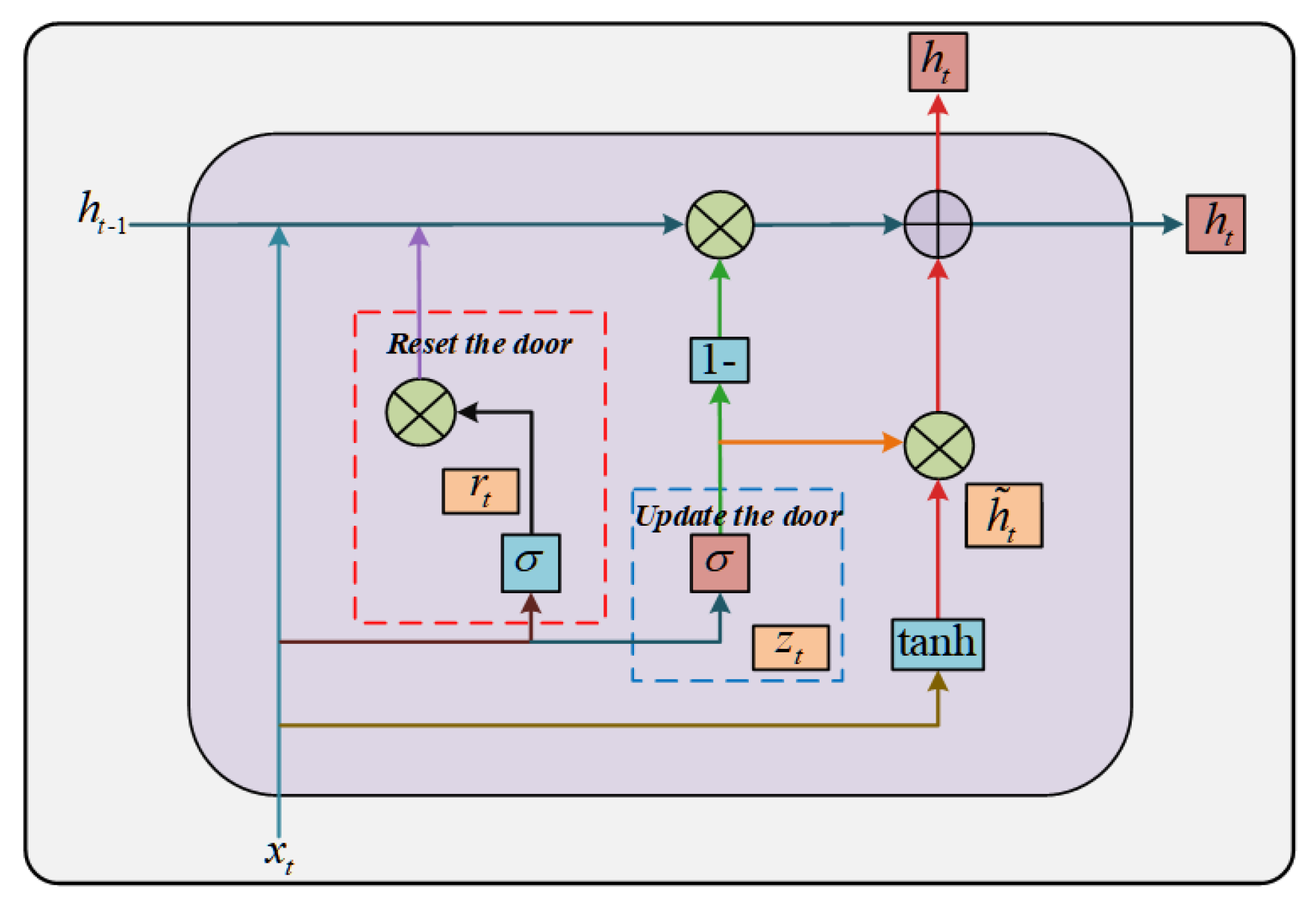
The GRU [33], a variant of the Recurrent Neural Network (RNN), introduces gate mechanisms to control the flow of information, effectively addressing the gradient vanishing and gradient exploding problems of traditional RNNs. Compared to LSTM, the GRU has a simpler structure and higher computational efficiency. The GRU is primarily controlled by two gates, the update gate and the reset gate, which manage the processes of feature learning update and forgetting, respectively. The GRU network structure is illustrated in Figure 2. Below are the detailed main computational formulas of the GRU:
Update Gate: This gate is primarily used to determine how much of the previous time step’s state should be retained. The specific internal mathematical operation is as follows:
z t = σ ( W z · [ h t 1 , x t ] )
σ ( x ) = 1 1 + e x
where x t represents the input value at the current time step, z t is the output of the update gate, W z is the corresponding weight vector, and h t 1 is the hidden state value from the previous time step. σ is the sigmoid activation function.
Reset Gate: This gate mainly controls how much state information has been reset in the previous moment. The specific internal mathematical operations are as follows:
r t = σ ( W r · [ h t 1 , x t ] )
where W r is the corresponding weight vector, r t represents the reset gate output value of time step t, and σ is the sigmoid activation function.
Hidden state: The hidden state has two values, one as the candidate hidden state value h ˜ t and the other as the final hidden state value h t . The current candidate hidden state value is completed by Formula (9), and the final hidden state value is completed by Formula (10). The specific internal mathematical operations are as follows:
h ˜ t = tanh ( W · [ r t h t 1 , x t ] )
h t = ( 1 z t ) h t 1 + z t h ˜ t
where W is the corresponding weight vector, and ⊙ is the product of elements.

3. Analysis of Experimental Process

3.1. CWRU Bearing Data Analysis

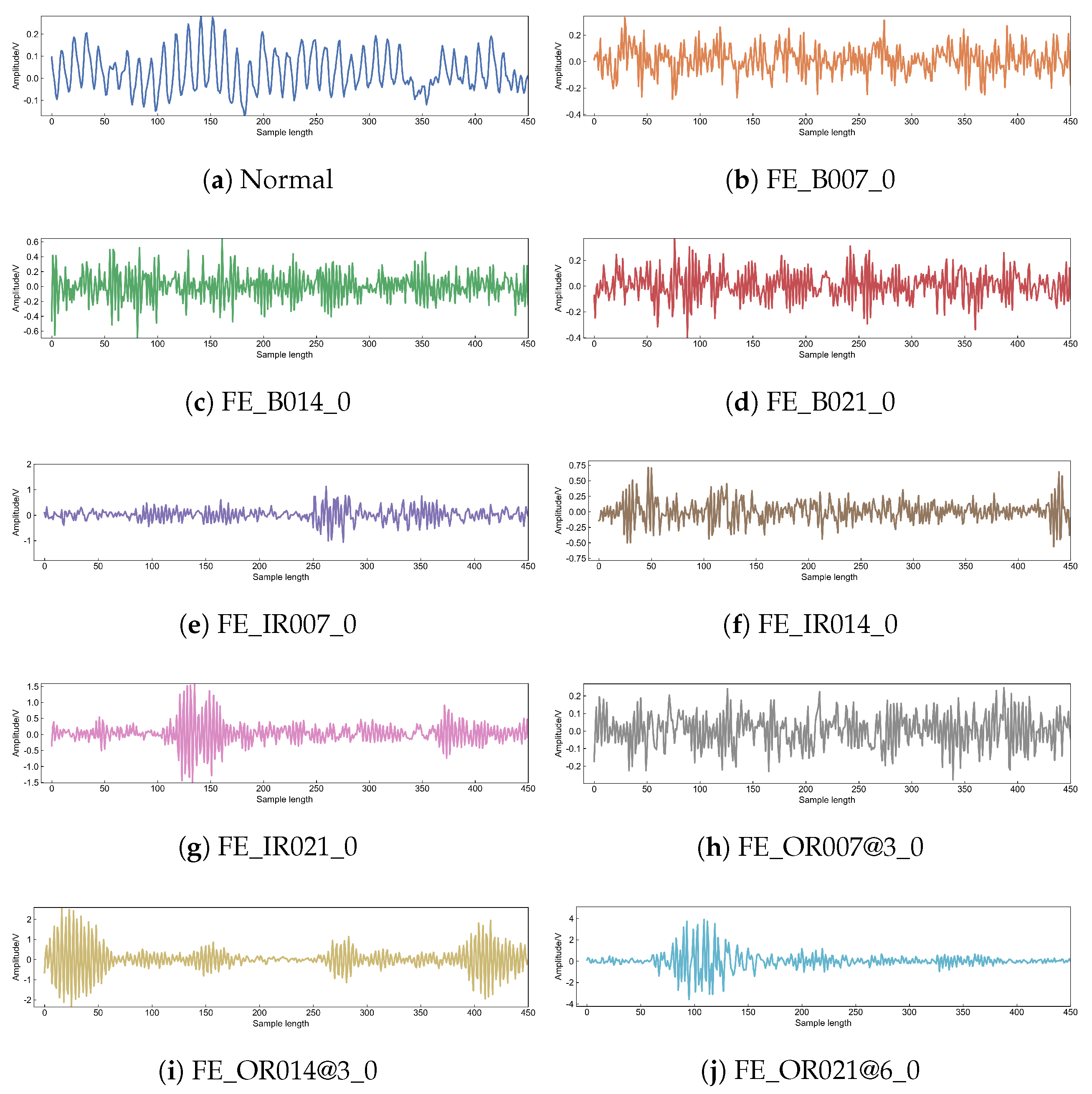
In this study, we use data from the Case Western Reserve University (CWRU) Bearing Data Center to validate the effectiveness of the proposed CNN-GRU method. It is publicly available at (https://engineering.case.edu/bearingdatacenter/apparatus-and-procedures (accessed on 8 December 2024). The specific bearing test rig, which consists of an electric motor coupled to a bearing housing with a rotating shaft, is shown in Figure 3. The data used in this study were collected by an accelerometer sensor mounted on the fan end of the motor housing, located in the 12 o’clock direction relative to the motor axis. The sensor records vibration signals at a data acquisition frequency of 12 kHz (12,000 samples per second), ensuring a high temporal resolution for capturing detailed fault characteristics. The motor operates under a no-load condition with a speed of 1797 rpm, which is the standard operating condition for this test rig. The no-load speed ensures that the observed vibrations are primarily caused by bearing defects rather than load-related factors, allowing for focused analysis of fault-induced signatures [34,35]. There are three fault types with different sizes: small (0.007 inches), medium (0.014 inches), and large (0.021 inches). For this experiment, we categorized the bearing data into 10 different classes: one normal bearing dataset, three datasets for inner race faults of varying sizes, three datasets for outer race faults of varying sizes, and three datasets for ball faults of varying sizes. The detailed data are shown in Table 2, and the initial bearing data curves for the 10 categories are illustrated in Figure 4. In Table 2 and Figure 4, “FE” denotes the fan end, “B” denotes the rolling element, “IR” denotes the inner race, and “OR” denotes the outer race. The numbers “007”, “014”, and “021” represent fault diameters of 0.007, 0.014, and 0.021, respectively. The symbols “@3” and “@6” indicate the relative position of the fault to the load zone in terms of clock direction, meaning the fault occurs at the three o’clock and six o’clock positions. The subscript “−0” signifies that the motor load is at 0 horsepower (HP) at that moment.

3.2. Filtering Process

Applying envelope analysis and adaptive mean filtering to bearing data can significantly improve the signal-to-noise ratio, making the useful signal components more prominent while removing irrelevant high-frequency noise. This simplified the bearing data and provided higher accuracy for our bearing fault diagnosis tasks, effectively ensuring the reliability and safety of equipment operation. In the process of envelope analysis and adaptive mean filtering, the envelope analysis was handled using the Hilbert transform function, while the adaptive mean filter was set with a window size of w 2 and a noise threshold t h of 0.5. The window size was chosen based on the trade-off between denoising effectiveness and signal fidelity, and the noise threshold controlled whether adaptive adjustment was needed.
To validate the effectiveness of combining envelope analysis with the adaptive mean filtering algorithm, we applied both the combined algorithm and the standalone adaptive mean filtering algorithm, and the results are presented in Figure 5. The left subgraph, labeled “single”, represents the standalone filtering algorithm, while the right subgraph, labeled “combine”, illustrates the combined filtering algorithm. By comparing the experimental results, we found that the combined filtering algorithm demonstrated significantly better performance, with key data fault features becoming more pronounced. This provides superior data support for subsequent fault diagnosis tasks.

3.3. Z-Score Standardization of Bearing Data

In the preliminary data processing stage, we applied Z-score normalization to the bearing data. This normalization technique transforms data of different magnitudes into dimensionless data, ensuring that each element of the bearing data has the same scale, with a mean of 0 and a standard deviation of 1. After this processing stage, the model can achieve better convergence, thereby accelerating the entire fault diagnosis process. The specific data computation for this process can be expressed as follows:
m = m n h
where m represents the standardized bearing data, and n and h represent the average and standard deviation of the original data, respectively.

3.4. Box Plot Analysis of Raw and Filtered Bearing Data

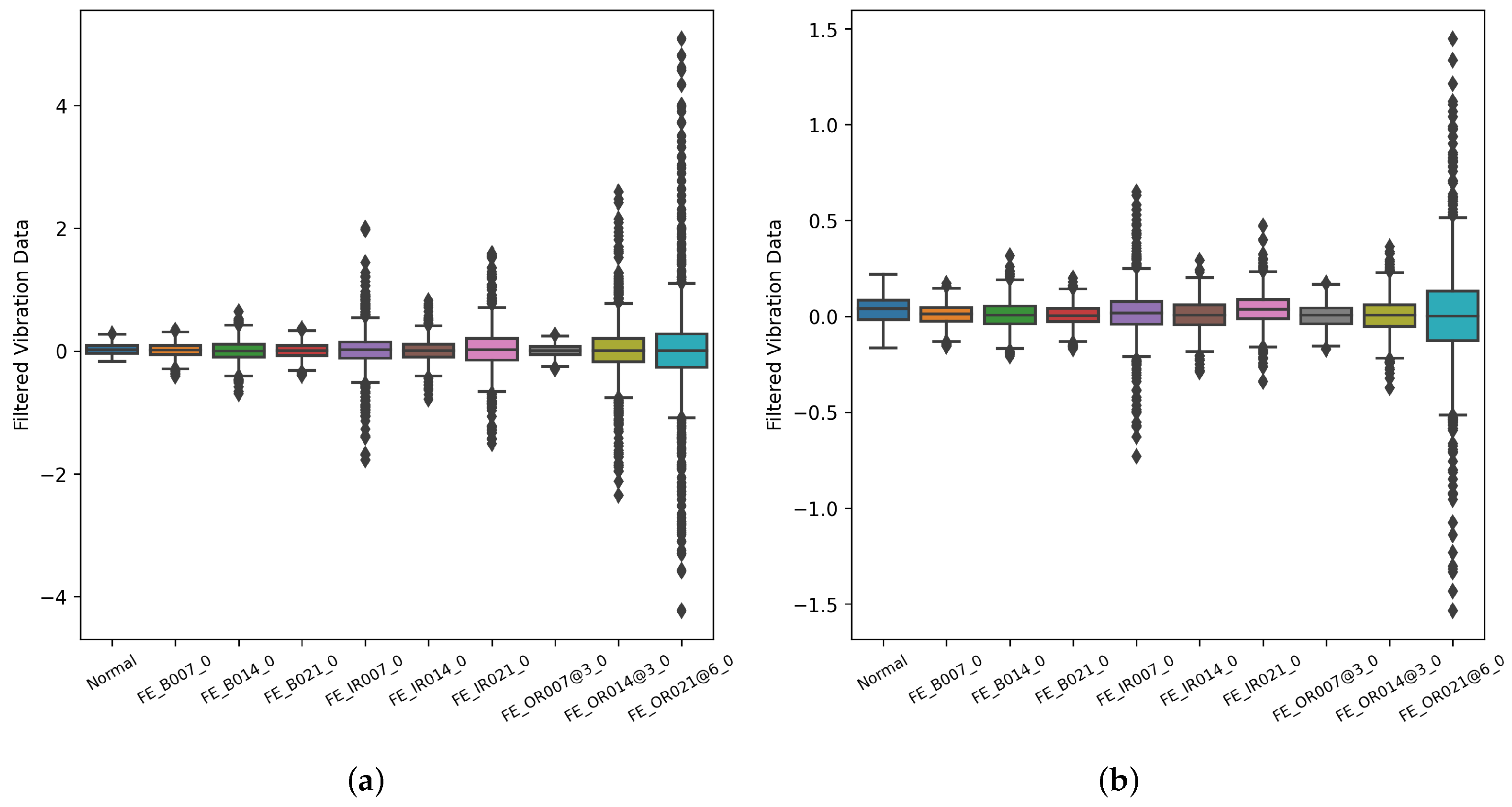
In this section, we use box plots to analyze the original and filtered bearing data. Box plots help visually demonstrate the central tendency and dispersion of different categories, as well as identify problematic values within the data. In Figure 6a, we observe that the original data distribution is relatively uniform. The data features of the Normal, FE-B007-0, and FE-OR007@3-0 categories are very similar and close to each other, making them difficult to distinguish, indicating the presence of noise and some outliers. However, in Figure 6b, we notice that the data distribution is more concentrated, the height of the boxes is reduced, and the number of outliers is decreased. This indicates that the noise has been effectively removed, resulting in smoother data.

3.5. Establishment of CNN GRU Fault Diagnosis Model

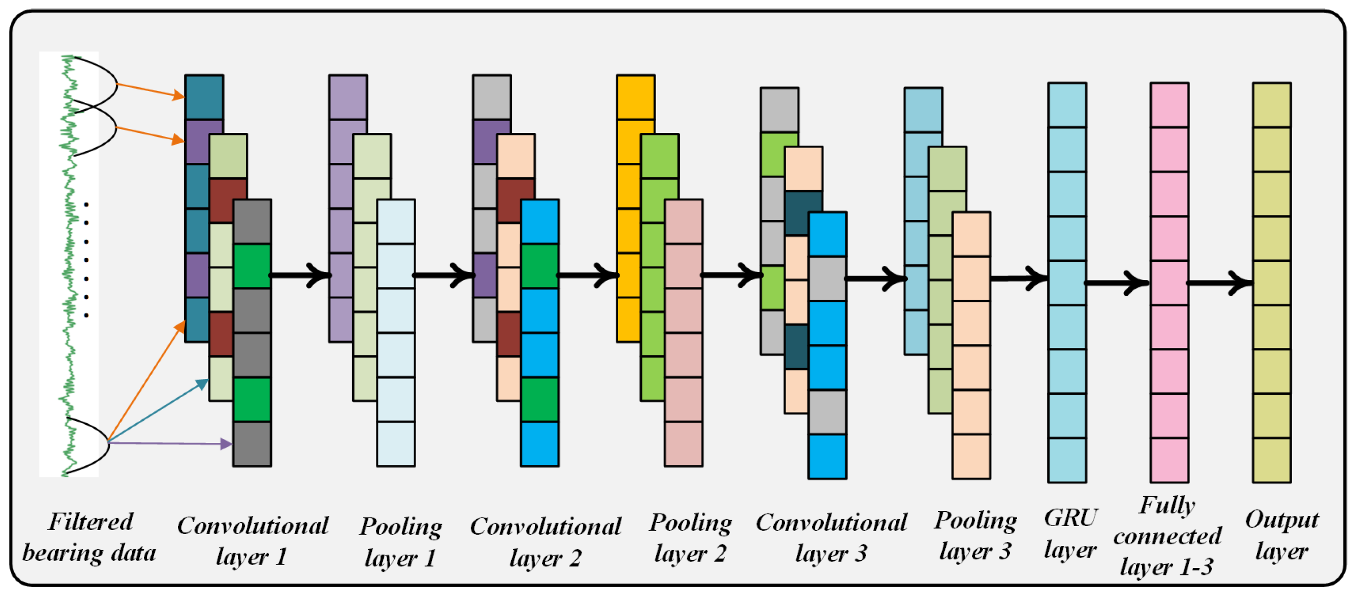
The CNN-GRU fault diagnosis model established in this study is shown in Figure 7. This combined diagnostic model efficiently extracts spatial features and temporal dependencies from the bearing data, providing accurate fault diagnosis results. As illustrated in Figure 7, the input data for the model are the filtered bearing data. The framework initially consists of three convolution-pooling alternating layers. The extracted features are then fed into the GRU layer for further feature learning and extraction. Finally, the features pass through three fully connected layers for refinement and enhancement. The output layer uses the Softmax function to compute the probability values. The specific parameters of the CNN-GRU model are organized in Table 3.
In this study, we propose a CNN-GRU model that uses a CNN to extract local features from the bearing data. Although the CNN performs convolution operations on the input data, it does not disrupt the temporal order. The convolutional operations of the CNN are applied to each time step, extracting local spatial features while preserving the original temporal structure without altering the sequence order. The extracted features are then fed into the GRU, which leverages these temporally preserved features to capture time dependencies. In this way, the local feature extraction by the CNN and the time dependency modeling by the GRU work together to ensure the model’s effectiveness in both spatial and temporal aspects.

3.6. Introduction to Experimental Equipment and Training Parameters

In this experiment, the computer’s operating system was Windows, with 8 GB of RAM. Additionally, a GIGABYTE GeForce GTX 1050 graphics card with 2 GB of DDR5 VRAM was used to accelerate the training of the neural network. The programming language used for this experiment was Python, specifically version 3.6, and the code editor employed was Pycharm 2021.
The deep learning framework used was PyTorch, which offers better understanding and flexibility during code development. In terms of model parameter design, the convolution kernel size of the first convolutional layer was set to 16, which helped cover a larger input area and better capture long-term dependencies in the input data. The alternating combination of three convolution-pooling layers allows the model to extract higher-level features step by step while effectively reducing the size of feature maps and the number of parameters, resulting in better feature learning.The inclusion of the GRU layer enables effective capturing of long-term dependencies in the time-series data. This allows the model to track changes and dependencies in the spatial features over time, enhancing the understanding of these features. The fully connected layers flatten the high-dimensional features output by the GRU layer into a one-dimensional vector. Through weight matrices and activation functions, the fully connected layers can perform nonlinear combinations of the features extracted by the GRU, thereby improving the fault diagnosis task.
During the model training process, the classification loss function used was the cross-entropy loss function. The optimizer adopted was Adam, known for its superior effectiveness. The learning rate decreased during training between 0.1 and 0.001. When inputting the model learning parameters, both small-batch sample data and labels were separately placed into CUDA for accelerated training, thereby providing faster training for us.

3.7. Model Training and Test Result Analysis

For data preprocessing, the dataset was divided into training, validation, and test sets with a ratio of 6:2:2, which ensured a balanced distribution of data across all subsets. Furthermore, during small-batch iterations, both the training and validation sets were shuffled to prevent any bias and to enhance the generalization ability of the model. This approach was particularly important in improving the model’s performance and robustness by ensuring that the training process does not overfit to any specific order of the data.

3.7.1. Model Training Analysis and Visualization Display

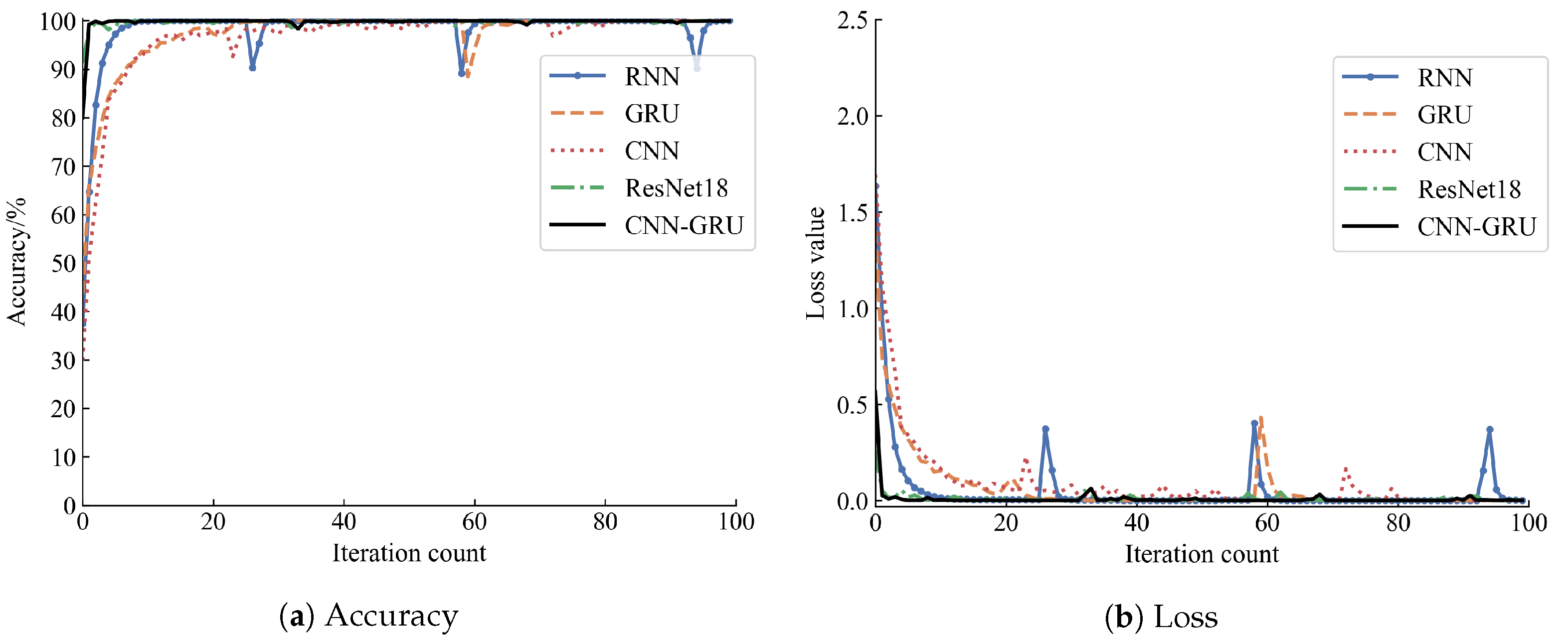
During the training of the CNN-GRU model, to visually demonstrate the advantages of the method proposed in this paper, we selected and validated four comparison methods: CNN [32], GRU [33], RNN [36], and ResNet18 [37], comparing their performance with CNN-GRU. The CNN excels in spatial feature extraction but lacks capability in handling temporal dependencies. The RNN and GRU have advantages in capturing temporal dependencies but are less effective in spatial feature extraction. ResNet18 is powerful in deep feature extraction but requires adjustments to suit time-series data. By comparing the accuracy and loss iteration curves of these five methods, we can clearly observe their performance differences. Figure 8 illustrates the training performance over 100 iterations: Figure 8a shows the accuracy iteration curve, and Figure 8b shows the loss iteration curve. From the figures, it is evident that the CNN-GRU model achieves faster accuracy improvement during training, ultimately reaching higher accuracy. Additionally, its loss reduction is more pronounced, validating its effectiveness and superiority in handling bearing fault diagnosis tasks.
In Figure 8a, the CNN-GRU model demonstrates rapid and stable convergence, showcasing robust performance. In contrast, the RNN model exhibits significant fluctuations during iterations, particularly around iterations 25, 60, and 93. The GRU model also shows fluctuations around iteration 60, but with a smaller amplitude, indicating its better capability in handling temporal dependencies. Overall, the CNN-GRU model exhibits more stable and rapid convergence during training compared to the RNN and GRU.
In Figure 8b, the CNN-GRU model exhibits a highly stable and excellent curve of loss variation, maintaining consistently low levels of loss. In comparison, ResNet18 shows some similarity in the trend of loss variation with CNN-GRU, but the ResNet18 model requires a longer training time. Both the RNN and GRU models display abrupt changes in loss during training, indicating unstable performance. Overall, the CNN-GRU model demonstrates outstanding stability in loss and convergence speed, showcasing more efficient training characteristics compared to ResNet18.

3.7.2. Model Testing Analysis and Visualization Display

In each iteration of training, we validated the learned model using a validation set and saved the optimal model. During testing, we loaded the saved weights and parameters from the optimal model, enabling us to evaluate our test set under the best feature learning parameters. This approach allowed us to analyze the performance of the five models on the test set effectively. To visually demonstrate the differentiation of bearing data across the ten categories under different fault diagnosis models, we utilize confusion matrices [38]. Figure 9 illustrates five confusion matrix graphs, where the horizontal axis represents the actual bearing fault categories, and the vertical axis represents the diagnostic categories predicted by different models. The diagonal elements of each category indicate the correct diagnosis rates, while the off-diagonal elements denote the misclassification rates. By examining the confusion matrices of the five models comprehensively, it is evident that our proposed CNN-GRU model achieves higher accuracy with minimal misclassifications and the highest correct diagnosis rates.
In Table 4, the average accuracies of the five models on the test set are displayed as follows: CNN-GRU performs the best, with an accuracy of 99.35%, yielding only a 0.65% error rate. In comparison, the RNN, the GRU, the CNN, and ResNet18 have average accuracies that are lower than CNN-GRU by 0.5%, 0.3%, 0.2%, and 0.05%, respectively. These figures clearly demonstrate the superiority of the CNN-GRU model in bearing fault diagnosis tasks. By combining the CNN’s capability to extract spatial features and the GRU’s ability to handle temporal dependencies, the CNN-GRU model effectively enhances diagnostic accuracy and stability.

3.7.3. T-SNE Visualization Analysis

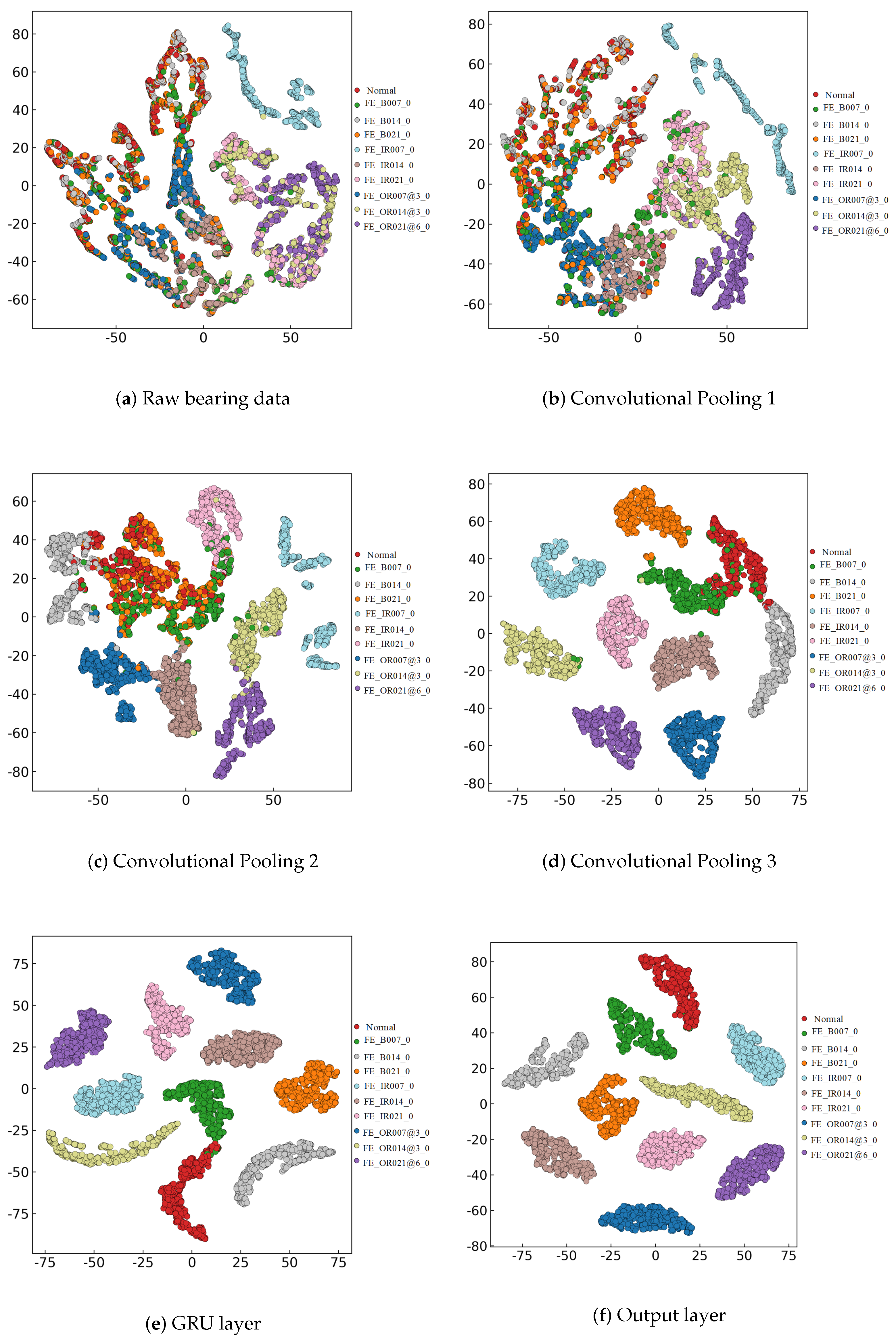
Due to the high-dimensional nature of both the original data and intermediate layer outputs in deep learning models, we chose to employ t-SNE [39] for dimensional reduction to two dimensions. This facilitated a clear and intuitive observation of bearing data classification, allowing us to evaluate the model’s effectiveness in distinguishing different data categories and thereby validating its performance. Initially, we visualized the original dataset after dimensionality reduction, as shown in Figure 10a. It reveals poor differentiation between different fault categories, with data points scattered chaotically. After feature extraction through three convolution-pooling layers (Figure 10b–d), the data features are progressively refined. With each convolution-pooling layer, feature extraction becomes more comprehensive, significantly reducing overlap among data points and enhancing differentiation between different categories. Following processing by the GRU layer (Figure 10e), the model further captures temporal dependencies in the data, demonstrating the GRU’s robust capability in extracting time-series features. Ultimately, in the visualization at the output layer (Figure 10f), the bearing data points from different fault types are almost completely separated, indicating optimal clustering. This showcases the powerful performance of the CNN-GRU model in bearing fault diagnosis tasks.
Through these t-SNE visualizations, we can intuitively observe the distributional changes in data across different layers, validating the effectiveness and superiority of the CNN-GRU model in feature extraction and classification.

4. Summary

Based on the noise issues in bearing data caused by environmental noise, sensor errors, and mechanical interference, this paper proposes a CNN-GRU rolling bearing fault diagnosis method based on adaptive filtering. The method was validated using the rolling bearing fan end dataset provided by CWRU. The experimental results demonstrate that the proposed method excels in denoising and fault feature extraction, effectively enhancing the accuracy and stability of fault diagnosis. The main conclusions drawn are as follows:
(1)
To address the issue of noise interference in bearing data, this paper applies envelope analysis and the adaptive mean filtering algorithm for denoising. The experimental results show that this method effectively highlights the main fault features, providing robust data preprocessing for fault diagnosis.
(2)
The combination of the CNN for spatial feature extraction and the GRU for temporal dependency modeling enables the proposed method to achieve high-precision fault diagnosis. Visualization techniques, such as confusion matrices and t-SNE, further demonstrate the diagnostic capabilities and generalization performance of the model.
(3)
Moving forward, we plan to explore the applicability of the proposed CNN-GRU model to other types of machinery and operational conditions to ensure robustness and scalability. Additionally, the integration of the model with real-time fault diagnosis systems and edge computing frameworks will be investigated to enhance its practical application value.

Author Contributions

Conceptualization, H.Z. and Z.S.; Methodology, H.Z. and Z.S.; Validation, J.X.; Formal Analysis, Z.S.; Resources, H.Z. and J.X.; Data Curation, Z.S.; Writing—Original Draft, J.X.; Writing—Review and Editing, Z.S. and Y.L.; Funding Acquisition, H.Z., J.X. and Y.L. All authors have read and agreed to the published version of the manuscript.

Funding

This study was funded by the Quzhou City Science and Technology Plan project (2023K263, 2023K265, 2023K045); the Public Welfare Technology Research Project of Zhejiang Province (under grant LGC22E050006); the General Research Project of Zhejiang Provincial Department of Education (2023) (Y202353440, Y202353289); and the Key project of Quzhou College of Technology (QZYZ2305).

Data Availability Statement

The data presented in this study are available in the article.

Conflicts of Interest

The authors declare no conflict of interest.

References

  1. AlShorman, O.; Irfan, M.; Saad, N.; Zhen, D.; Haider, N.; Glowacz, A.; AlShorman, A. A review of artificial intelligence methods for condition monitoring and fault diagnosis of rolling element bearings for induction motor. Shock Vib. 2020, 2020, 8843759. [Google Scholar] [CrossRef]
  2. Salunkhe, V.G.; Khot, S.M.; Jadhav, P.S.; Yelve, N.P.; Kumbhar, M.B. Experimental investigation using robust deep VMD-ICA and 1D-CNN for condition monitoring of roller element bearing. J. Comput. Inf. Sci. Eng. 2024, 24, 124501. [Google Scholar] [CrossRef]
  3. Pan, Z.; Meng, Z.; Chen, Z.; Gao, W.; Shi, Y. A two-stage method based on extreme learning machine for predicting the remaining useful life of rolling-element bearings. Mech. Syst. Signal Process. 2020, 144, 106899. [Google Scholar] [CrossRef]
  4. Liu, Z.; Zhang, L. A review of failure modes, condition monitoring and fault diagnosis methods for large-scale wind turbine bearings. Measurement 2020, 149, 107002. [Google Scholar] [CrossRef]
  5. Wu, Z.H.; Xu, Y.Q.; Deng, S.E. Analysis of Dynamic Characteristics of Grease-Lubricated Tapered Roller Bearings. Shock Vib. 2018, 2018, 7183042. [Google Scholar] [CrossRef]
  6. Dhanola, A.; Garg, H.C. Tribological challenges and advancements in wind turbine bearings: A review. Eng. Fail. Anal. 2020, 118, 104885. [Google Scholar] [CrossRef]
  7. Su, Y.; Shi, L.; Zhou, K.; Bai, G.; Wang, Z. Knowledge-informed deep networks for robust fault diagnosis of rolling bearings. Reliab. Eng. Syst. Saf. 2024, 244, 109863. [Google Scholar] [CrossRef]
  8. Liu, Y.; Ma, G.; Qin, H.; Han, C.; Shi, J. Research on damage and failure behaviour of coated self-lubricating spherical plain bearings based on detection of friction torque and temperature rise. Proc. Inst. Mech. Eng. Part J Eng. Tribol. 2022, 236, 514–526. [Google Scholar] [CrossRef]
  9. Salunkhe, V.G.; Khot, S.M.; Desavale, R.; Yelve, N. Unbalance Bearing Fault Identification Using Highly Accurate Hilbert-Huang Transform Approach. J. Nondestruct. Eval. Diagn. Progn. Eng. Syst. 2023, 6, 031005. [Google Scholar] [CrossRef]
  10. Brkovic, A.; Gajic, D.; Gligorijevic, J.; Savic-Gajic, I.; Georgieva, O.; Di Gennaro, S. Early fault detection and diagnosis in bearings for more efficient operation of rotating machinery. Energy 2017, 136, 63–71. [Google Scholar] [CrossRef]
  11. Salunkhe, V.G.; Desavale, R.G.; Khot, S.M.; Yelve, N.P. A Novel Incipient Fault Detection Technique for Roller Bearing Using Deep Independent Component Analysis and Variational Modal Decomposition. J. Tribol. 2023, 145, 074301. [Google Scholar] [CrossRef]
  12. Hamadache, M.; Jung, J.H.; Park, J.; Youn, B.D. A comprehensive review of artificial intelligence-based approaches for rolling element bearing PHM: Shallow and deep learning. JMST Adv. 2019, 1, 125–151. [Google Scholar] [CrossRef]
  13. Zio, E. Some challenges and opportunities in reliability engineering. IEEE Trans. Reliab. 2016, 65, 1769–1782. [Google Scholar] [CrossRef]
  14. Zhen, D.; Guo, J.; Xu, Y.; Zhang, H.; Gu, F. A novel fault detection method for rolling bearings based on non-stationary vibration signature analysis. Sensors 2019, 19, 3994. [Google Scholar] [CrossRef] [PubMed]
  15. Berrouche, Y. A Non-Parametric Empirical Method for Nonlinear and Non-Stationary Signal Analysis. Eng. Technol. Appl. Sci. Res. 2022, 12, 8058–8062. [Google Scholar] [CrossRef]
  16. Islam, M.M.; Kim, J.M. Automated bearing fault diagnosis scheme using 2D representation of wavelet packet transform and deep convolutional neural network. Comput. Ind. 2019, 106, 142–153. [Google Scholar] [CrossRef]
  17. He, M.; He, D. Deep learning based approach for bearing fault diagnosis. IEEE Trans. Ind. Appl. 2017, 53, 3057–3065. [Google Scholar] [CrossRef]
  18. Yu, X.; Dong, F.; Ding, E.; Wu, S.; Fan, C. Rolling bearing fault diagnosis using modified LFDA and EMD with sensitive feature selection. IEEE Access 2017, 6, 3715–3730. [Google Scholar] [CrossRef]
  19. Yuan, L.; Lian, D.; Kang, X.; Chen, Y.; Zhai, K. Rolling bearing fault diagnosis based on convolutional neural network and support vector machine. IEEE Access 2020, 8, 137395–137406. [Google Scholar] [CrossRef]
  20. Li, H.; Liu, T.; Wu, X.; Chen, Q. An optimized VMD method and its applications in bearing fault diagnosis. Measurement 2020, 166, 108185. [Google Scholar] [CrossRef]
  21. Shi, Z.; Zhang, G.; Liu, J.; Li, X.; Xu, Y.; Yan, C. Influences of inclined crack defects on vibration characteristics of cylindrical roller bearings. Mech. Syst. Signal Process. 2024, 207, 110945. [Google Scholar] [CrossRef]
  22. Zhou, F.; Gao, Y.; Wen, C. A novel multimode fault classification method based on deep learning. J. Control. Sci. Eng. 2017, 2017, 3583610. [Google Scholar] [CrossRef]
  23. Yang, S.; Tang, B.; Wang, W.; Yang, Q.; Hu, C. Physics-informed multi-state temporal frequency network for RUL prediction of rolling bearings. Reliab. Eng. Syst. Saf. 2024, 242, 109716. [Google Scholar] [CrossRef]
  24. Sohaib, M.; Kim, J.M. Reliable fault diagnosis of rotary machine bearings using a stacked sparse autoencoder-based deep neural network. Shock Vib. 2018, 2018, 2919637. [Google Scholar] [CrossRef]
  25. Chen, X.; Zhang, B.; Gao, D. Bearing fault diagnosis base on multi-scale CNN and LSTM model. J. Intell. Manuf. 2021, 32, 971–987. [Google Scholar] [CrossRef]
  26. Chen, J.; Jiang, J.; Guo, X.; Tan, L. A self-Adaptive CNN with PSO for bearing fault diagnosis. Syst. Sci. Control. Eng. 2021, 9, 11–22. [Google Scholar] [CrossRef]
  27. Han, T.; Zhang, L.; Yin, Z.; Tan, A.C. Rolling bearing fault diagnosis with combined convolutional neural networks and support vector machine. Measurement 2021, 177, 109022. [Google Scholar] [CrossRef]
  28. Tao, H.; Qiu, J.; Chen, Y.; Stojanovic, V.; Cheng, L. Unsupervised cross-domain rolling bearing fault diagnosis based on time-frequency information fusion. J. Frankl. Inst. 2023, 360, 1454–1477. [Google Scholar] [CrossRef]
  29. Huang, Y.J.; Liao, A.H.; Hu, D.Y.; Shi, W.; Zheng, S.B. Multi-scale convolutional network with channel attention mechanism for rolling bearing fault diagnosis. Measurement 2022, 203, 111935. [Google Scholar] [CrossRef]
  30. Salunkhe, V.G.; Khot, S.M.; Desavale, R.G.; Yelve, N.P.; Jadhav, P.S. An Integrated Dimension Theory and Modulation Signal Bispectrum Technique for Analyzing Bearing Fault in Industrial Fibrizer. J. Nondestruct. Eval. Diagn. Progn. Eng. Syst. 2024, 7, 031006. [Google Scholar] [CrossRef]
  31. Xu, T.; You, J.; Li, H.; Shao, L. Energy efficiency evaluation based on data envelopment analysis: A literature review. Energies 2020, 13, 3548. [Google Scholar] [CrossRef]
  32. Eren, L.; Ince, T.; Kiranyaz, S. A generic intelligent bearing fault diagnosis system using compact adaptive 1D CNN classifier. J. Signal Process. Syst. 2019, 91, 179–189. [Google Scholar] [CrossRef]
  33. Xu, J.; Sui, Z.; Wang, W.; Xu, F. An Adaptive Discrete Integral Terminal Sliding Mode Control Method for a Two-Joint Manipulator. Processes 2024, 12, 1106. [Google Scholar] [CrossRef]
  34. Xu, F.; Sui, Z.; Ye, J.; Xu, J. Ternary Precursor Centrifuge Rolling Bearing Fault Diagnosis Based on Adaptive Sample Length Adjustment of 1DCNN-SeNet. Processes 2024, 12, 702. [Google Scholar] [CrossRef]
  35. Yuan, J.; Tian, Y. An intelligent fault diagnosis method using GRU neural network towards sequential data in dynamic processes. Processes 2019, 7, 152. [Google Scholar] [CrossRef]
  36. Zhu, J.; Jiang, Q.; Shen, Y.; Qian, C.; Xu, F.; Zhu, Q. Application of recurrent neural network to mechanical fault diagnosis: A review. J. Mech. Sci. Technol. 2022, 36, 527–542. [Google Scholar] [CrossRef]
  37. Wei, D.; Liu, K.; Wang, J.; Zhou, S.; Li, K. ResNet-18 based Inter-turn Short Circuit Fault Diagnosis of PMSMs with Consideration of Speed and Current Loop Bandwidths. IEEE Trans. Transp. Electrif. 2023, 10, 5805–5818. [Google Scholar] [CrossRef]
  38. Salunkhe, V.G.; Desavale, R.; Khot, S.M.; Yelve, N. Identification of Bearing Clearance in Sugar Centrifuge Using Dimension Theory and Support Vector Machine on Vibration Measurement. J. Nondestruct. Eval. Diagn. Progn. Eng. Syst. 2024, 7, 021003. [Google Scholar] [CrossRef]
  39. Lee, C.Y.; Lin, W.C. Induction motor fault classification based on ROC curve and t-SNE. IEEE Access 2021, 9, 56330–56343. [Google Scholar] [CrossRef]
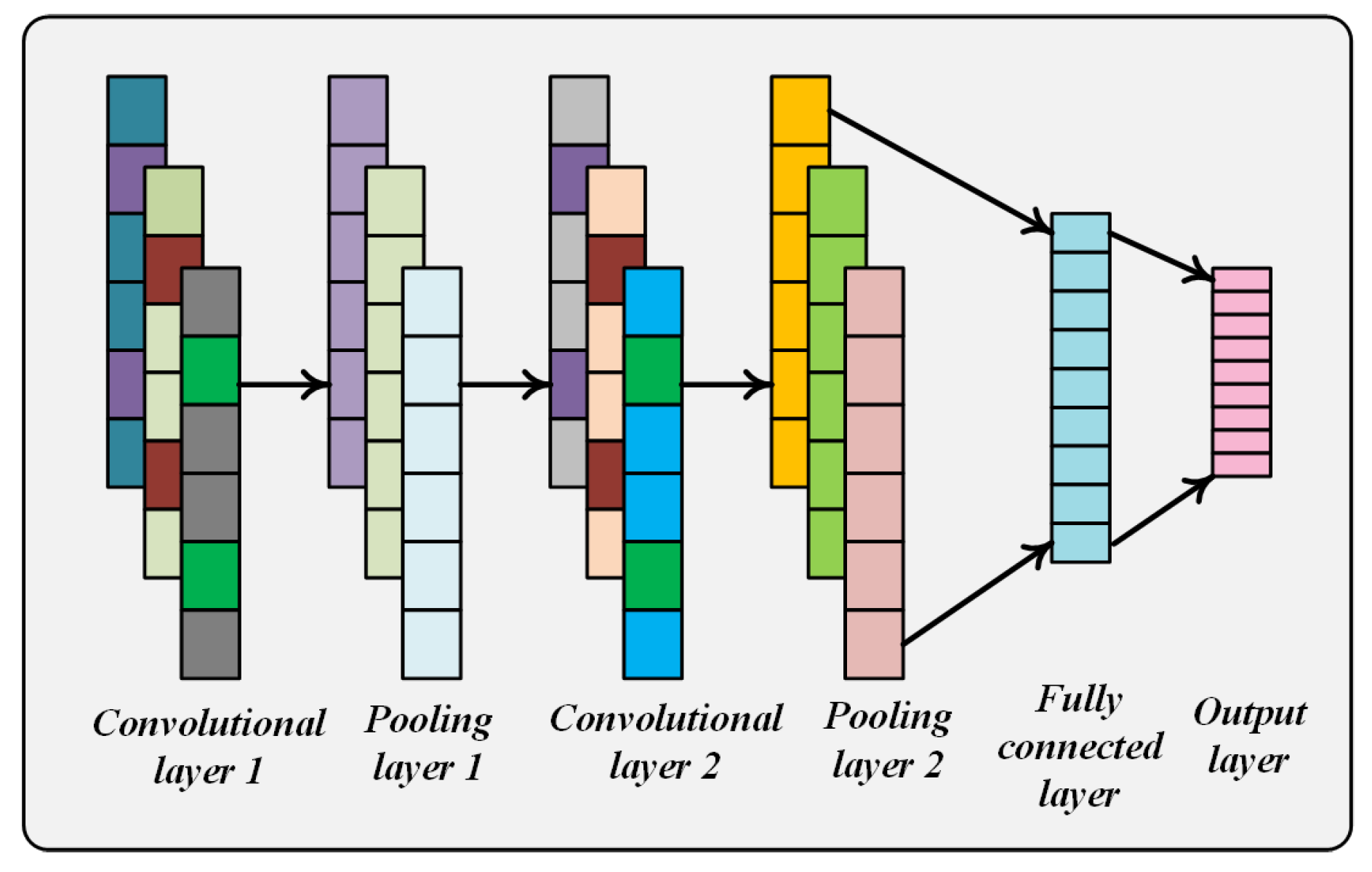
Figure 1. CNN structure diagram.
Processes 12 02845 g001
Figure 2. GRU network structure diagram.
Processes 12 02845 g002
Figure 3. Experimental diagram of CWRU bearing equipment.
Processes 12 02845 g003
Figure 4. Initial data curve of bearings.
Processes 12 02845 g004
Figure 5. Comparison results of different filtering algorithms for bearings.
Processes 12 02845 g005
Figure 6. Box plot of 10 categories of bearing data ((a) original bearing data; (b) filtered bearing data).
Processes 12 02845 g006
Figure 7. CNN-GRU fault diagnosis model.
Processes 12 02845 g007
Figure 8. Accuracy and loss value variation curve during training process.
Processes 12 02845 g008
Figure 9. A visual display of the confusion matrix in the test set.
Processes 12 02845 g009aProcesses 12 02845 g009b
Figure 10. Visualization of t-SNE clustering in different processes of the model.
Processes 12 02845 g010
Table 1. Acronyms and their meanings.
AcronymMeaning
CNNConvolutional Neural Network
GRUGated Recurrent Unit
LSTMLong short-term memory
VMDVariational mode decomposition
RNNRecurrent Neural Network
CWRUCase Western Reserve University
FEFan end
BRolling element
IRInner race
OROuter race
HPHorsepower
Table 2. Data of 10 different categories of bearings.
Data NameFault SizeApplied LoadSpeedSample ShapeFault Label
Normal bearings0HP1797rpm1000 × 1024Normal
Ball damage fault0.007 inch0 HP1797 rpm1000 × 1024FE_B007_0
Ball damage fault0.014 inch0 HP1797 rpm1000 × 1024FE_B014_0
Ball damage fault0.021 inch0 HP1797 rpm1000 × 1024FE_B021_0
Inner damage fault0.007 inch0 HP1797 rpm1000 × 1024FE_IR007_0
Inner damage fault0.014 inch0 HP1797 rpm1000 × 1024FE_IR014_0
Inner damage fault0.021 inch0 HP1797 rpm1000 × 1024FE_IR021_0
Outer damage fault0.007 inch0 HP1797 rpm1000 × 1024FE_OR007@3_0
Outer damage fault0.014 inch0 HP1797 rpm1000 × 1024FE_OR014@3_0
Outer damage fault0.021 inch0 HP1797 rpm1000 × 1024FE_OR021@6_0
Table 3. Specific parameters of CNN-GRU model.
Network Layer NameNumber of Output ChannelsConvolutional Kernel Size wFill SizeStrideActivation FunctionOutput Size
Conv 164(16,1)(1,1)(1,1)ReLU64@1 × 259
Pooling 164(2,1)(2,1)64@1 × 129
Conv 232(3,1)(1,1)(1,1)ReLU32@1 × 127
Pooling 232(2,1)(2,1)32@1 × 63
Conv 332(3,1)(1,1)(1,1)ReLU32@1 × 62
Pooling 332(2,1)(2,1)32@1 × 30
GRU 1128tanh1 × 128
GRU 2256tanh1 × 256
FC 11000ReLU1000
FC 2100ReLU100
FC 310Softmax10
Output1010
Table 4. Average testing accuracy of different models.
Diagnostic ModelAverage Accuracy %Average Error Rate %
RNN98.851.15
GRU99.050.95
CNN99.150.85
ResNet1899.300.70
CNN-GRU99.350.65
Disclaimer/Publisher’s Note: The statements, opinions and data contained in all publications are solely those of the individual author(s) and contributor(s) and not of MDPI and/or the editor(s). MDPI and/or the editor(s) disclaim responsibility for any injury to people or property resulting from any ideas, methods, instructions or products referred to in the content.