Abstract
In the field of industrial equipment reliability assessment, dependency on either degradation or failure time data is common. However, practical applications often reveal that single-type reliability data for certain industrial equipment are insufficient for a comprehensive assessment. This paper introduces a Bayesian-fusion-based methodology to enhance the reliability assessment of industrial equipment. Operating within the hierarchical Bayesian framework, the method innovatively combines the Wiener process with available degradation and failure time data. It further integrates a random effects model to capture individual differences among equipment units. The robustness and applicability of this proposed method are substantiated through an in-depth case study analysis.
1. Introduction
In sectors like energy, transportation, aviation, and aerospace, there is the extensive use of long-life industrial equipment [1,2,3]. These devices are pivotal, handling substantial workloads. Consequently, the assurance of their safe and reliable performance is a shared objective and necessity for both research and development entities and end-users [4,5,6].
The assessment of reliability has become central to the development of failure prevention and maintenance strategies for these devices [7,8]. Accurate reliability assessments enable the effective prediction of potential failures, thereby preventing equipment breakdowns and the subsequent significant economic losses. Traditional reliability assessment approaches depend on failure time data, which are represented through diverse statistical distribution models to convey the product’s reliability information over time. This type of data is typically acquired from field reliability tests, laboratory experiments, or after-sales service reports [9]. However, the extended lifespans of long-life industrial equipment result in infrequent failures, leading to a scarcity of failure time data. This scarcity poses substantial challenges to traditional reliability assessment methods that rely on such data, diminishing their applicability in practical scenarios [10].
In acknowledgement of these challenges, both industrial and academic sectors are increasingly focused on developing more advanced methods for the reliability assessment of long-life industrial equipment. A prominent example of such methods is analysis based on degradation data, which has become a vital component in the reliability assessment of such equipment [11,12,13,14,15]. This approach concentrates on the gradual deterioration of equipment performance indicators, which can often signal impending failures. Equipment performance inevitably degrades over time due to a combination of internal and external factors. This degradation occurs in a random pattern, influenced by variables such as environmental conditions, operational modes, and maintenance strategies. To capture and analyze this complex phenomenon with greater precision, stochastic processes are extensively employed. These processes facilitate a more accurate simulation and analysis of equipment performance degradation. Wiener-process-based models are especially effective in this area, as they precisely depict and predict the degradation trajectories of performance indicators [16]. The adaptability and robustness of these Wiener process models have fostered their extensive research and application in degradation analysis, significantly enhancing the reliability assessment of long-life industrial equipment. Wang et al. [17] explored real-time reliability assessment employing a generalized Wiener-process-based degradation model. They introduced a two-stage parameter estimation method along with adaptive evaluation procedures. Li et al. [18] formulated a reliability modeling approach for satellite momentum wheels utilizing an EM-based Wiener degradation model. This method efficiently estimates model parameters and was validated using specific degradation data. Gao et al. [19] proposed a multi-phase Wiener degradation process model tailored for systems with varying failure thresholds and drift parameters. They provided analytical solutions for assessing reliability in dynamic environments. Wang et al. [20] investigated the impact of inaccuracies in specifying nonlinear Wiener-process-based degradation models on product reliability assessment. Through a fatigue crack case study, they demonstrated that such discrepancies significantly influence mean-time-to-failure estimates. Li et al. [21] introduced a sequential Bayesian updated Wiener process model to enhance remaining useful life (RUL) prediction, employing comprehensive degradation data history for more precise drift parameter updates. Hu et al. [22] devised a real-time RUL prediction method for wind turbine bearings, utilizing a Wiener-process-based performance degradation model. Dai et al. [23] developed a reliability evaluation model for rolling bearings that integrates WaveletKernelNet, a bidirectional gated recurrent unit, and a Wiener process. This innovative method employs WKN-BiGRU for deep feature extraction and health index development, as well as the Wiener process for degradation modeling and uncertainty quantification in reliability assessments, corroborated by a real-case study. Liu et al. [24] merged an artificial neural network with a Wiener process, enhancing reliability estimation from accelerated testing data. This combination improved the accuracy in degradation modeling and life predictions, as confirmed by simulations and a stress relaxation case study. Guan et al. [25] developed a Wiener-process-based RUL prediction method that accounts for parameter dependency on operating conditions, thereby enhancing prediction accuracy. Shi et al. [26] introduced a reliability estimation method that combines a two-phase Wiener process with an evidential variable. This approach significantly improves accuracy in modeling two-phase degradation patterns, as demonstrated by both simulation and practical case studies. Lin et al. [27] proposed a nonlinear multi-phase Wiener process model for RUL prediction, integrating a stage division method with variational Bayesian parameter estimation. Zhang et al. [28] developed a lifetime estimation method for multi-component systems with degrading spare parts, employing Wiener-process-based models under both unit-by-unit and batch-by-batch replacement policies. Ma et al. [29] introduced a multi-phase Wiener-process-based degradation model that considers the impact of imperfect maintenance activities, utilizing a beta distribution for residual degradation and maximum likelihood estimation with Newton iteration for hyper-parameter estimation. Yan et al. [30] developed a multivariate correlated Wiener process model for the RUL prediction of products with multiple performance characteristics.
Industrial equipment, even of the same model and batch, often shows significant individual differences in reliability [31,32,33]. These differences originate from production uncertainties, including minor variations in material properties, fluctuations in processing precision, and slight assembly errors. Operational conditions and service environments also contribute to these individual differences. While seemingly minor at a macroscopic level, these subtle differences can, over time, result in substantial variations in the degradation characteristics among devices from the same production batch. Therefore, these individual differences, though they may seem minor at the level of single units, are crucial in the overall assessment of equipment reliability [34,35].
In the realm of reliability estimation based on degradation data, accurately accounting for individual differences in industrial equipment is essential. Neglecting or oversimplifying these differences results in unreliable estimates, which can adversely affect maintenance planning and risk management [36,37,38,39,40]. Enhancing the accuracy of these estimates necessitates incorporating each equipment’s unique characteristics into the model. A common method to tackle this challenge is the integration of random effects models into stochastic process models. These models enable certain parameters within the stochastic process to conform to specific probability distributions, thereby allowing for a more adaptable depiction and the prediction of each equipment’s degradation process. This approach more accurately captures individual differences [41,42]. Stochastic process models with random effects have gained widespread use in industrial reliability estimation for their efficiency in handling individual variability. These models not only provide more precise and reliable estimates but also lay a solid foundation for developing maintenance strategies and risk assessments. Wang [43] explored maximum likelihood inference for Wiener processes with random effects in degradation data analysis, accommodating unit-to-unit variability. This method employs the EM algorithm for parameter estimation, providing established asymptotic properties and uncertainty assessment via bootstrapping. Hao et al. [44] developed a Bayesian framework for reliability assessment, merging population and individual data. They used a Wiener process with random effects and MCMC for complex parameter estimation, demonstrating the effectiveness of Bayesian updating with a laser data case study. Pan et al. [45] proposed a reliability analysis model using a Wiener process with a truncated normal distribution, addressing unit-to-unit variability in scenarios where traditional normal distribution models are inadequate, such as in train wheel degradation. Zhai et al. [46] introduced a random-effects Wiener process model for product degradation, employing an inverse Gaussian distribution to handle unit-specific heterogeneity. This model, enhancing flexibility in the degradation rate and its variability correlation, was validated with laser and LED datasets for single-stress and multi-level accelerated degradation testing data. Wang et al. [47] developed a generalized Wiener-process-based degradation model with skew-normal random effects, using the EM algorithm and Bayesian updates for accurate residual life estimation. Duan et al. [48] presented an accelerated Wiener process model for RUL evaluation, integrating mixed random effects and measurement errors, validated with stress relaxation data. Wang et al. [49] proposed a Wiener-process-based reliability analysis method for accelerated degradation data, tailored for small samples and including unit variability testing. Zheng et al. [50] introduced an optimal acceptance sampling plan design for degraded products subjected to a Wiener process, optimizing test time and sample size while simplifying acceptance testing with the average degradation rate index. Yan et al. [51] offered a Wiener process model for left-truncated degradation data, incorporating random drift diffusion effects for precise RUL prediction and validated in practical applications. Tang et al. [52] suggested an unbiased parameter estimation method for Wiener-process-based degradation models, improving RUL prediction accuracy. This method, outperforming others in small sample sizes and model accuracy, addresses mis-specification challenges. Hou et al. [53] developed an enhanced random effects Wiener process model for lithium-ion battery reliability assessment, which is especially beneficial for limited sample sizes and long life cycles.
The Bayesian method has gained prominence in reliability assessment due to its effective use of historical and real-time observational data. This method’s primary strength is its capacity to manage uncertainty, enhancing the precision of reliability estimates by incorporating new data into existing prior information [54,55,56,57]. Consequently, it is frequently used to estimate unknown parameters in degradation models, particularly when these parameters exhibit complex distributions or are not directly measurable [58].
In practical applications of the Bayesian method for reliability estimation, a common challenge is the lack of comprehensive prior information. This issue is especially prevalent in assessing the reliability of new or upgraded industrial equipment, which often lacks extensive historical data [59,60,61,62]. A proven solution is to employ the Bayesian method to amalgamate diverse data types, including degradation and failure time data, recognized as multi-source heterogeneous data. Such integration not only maximizes data usage but also bolsters the reliability and precision of the estimates [63]. Pan [64] introduced a Bayesian approach for predicting product reliability, integrating field failure data with accelerated life test results and employing a calibration factor to address field stress uncertainty, as demonstrated with an electronic device case study. Wang et al. [65] developed a Bayesian method that combines accelerated degradation testing and field data for reliability evaluation. They used calibration factors and the Wiener process to align laboratory and field condition data, aiming for more precise real-world reliability predictions. Zhao et al. [66] presented a Bayesian method for estimating the residual life of Weibull-distributed satellite components, enhancing accuracy through multi-source information fusion, as shown in Monte Carlo simulations and a satellite momentum wheel case study. Wang et al. [67] developed Bayesian inference models to integrate diverse data types—Bernoulli, lifetime, and degradation—from multiple sources for comprehensive product reliability evaluation. Chen et al. [68] proposed a reliability estimation model for mechanical components, combining inverse Gaussian processes and copulas to merge degradation and failure time data. Validated through a case study and simulations, this model improves accuracy by accounting for dependencies among multiple performance indicators. Guo et al. [69] introduced a Bayesian information fusion approach for reliability analysis which integrates failure time and degradation data, and is notably effective for small samples. This method involves selecting the most suitable model from Wiener, gamma, and inverse Gaussian processes, using Markov chain Monte Carlo (MCMC) for parameter estimation. Chen et al. [70] proposed a technique to integrate multi-source accelerated degradation testing datasets, tackling disparities and epistemic uncertainties in degradation analysis. This method evaluates dataset quality and employs an uncertain degradation model to minimize analysis uncertainties, proven effective in simulation studies and practical applications. Kang et al. [71] focused on the reliability analysis of electronic devices using small-sample-size degradation data, integrated with historical data through a Wiener process. Their method, which considers consistent failure mechanisms across different data sets, demonstrated improved reliability estimation in both simulations and a real-world application to MOSFET degradation data. It is important to note that existing studies on data fusion have overlooked the individual variability present across different samples.
In high-precision engineering, dependence on degradation data for reliability analysis often falls short of meeting rigorous standards. Degradation data, while providing insight into equipment performance decline, may not comprehensively reflect all reliability-influencing factors, particularly with limited data [72,73,74,75,76]. To address this, we propose a novel Bayesian information fusion method for more accurate reliability analysis, especially effective in situations with small data samples. The uniqueness of this method lies in its integration of both traditional failure time data and degradation data. This integration yields a more holistic view of the factors impacting equipment performance and lifespan, enhancing the precision and trustworthiness of reliability evaluations. Additionally, the method incorporates a random effects model. This model accounts for variations among different devices or components, offering a nuanced understanding of individual differences. By employing this method, we can predict and mitigate potential equipment failures more effectively. Consequently, this approach significantly boosts production efficiency and elevates the safety and reliability of the equipment.
2. Theoretical Foundation
2.1. Wiener Process Model
We can assume that the degradation process of a selected performance indicator follows a Wiener process, which can be expressed as:
where is the drift parameter reflecting the degradation rate, is the diffusion parameter, and represents the standard Brownian motion process depicting the degradation process’s random dynamics.
Characteristics of the Wiener process used to represent the degradation process include:
- (1)
- ;
- (2)
- Independent increments;
- (3)
- The notion that these increments follow a normal distribution.
The probability density function of degradation increments can be represented as:
Since degradation increments can be non-positive, the Wiener process can describe non-monotonic degradation processes. The Wiener process offers significantly broader applicability than the Gamma process and the inverse Gaussian model, which are limited to describing monotonic degradation processes. This versatility becomes particularly relevant in the context of complex electromechanical products, like aircraft engines, where degradation indicators often exhibit non-monotonic behavior. In these instances, the Wiener process proves to be an effective tool for accurately characterizing the nuances of the degradation process [77].
Defining a failure threshold for the degradation process, the first time passage (also described as the product’s failure time) can be expressed as:
According to the basic properties of the Wiener process and the definition of first passage time, it follows an inverse Gaussian distribution: . When , the degradation process is a linear Wiener process, and the first passage time is given by: . The corresponding probability density function (PDF) and reliability function, respectively, are:
2.2. Wiener Process Model Considering Individual Differences
In numerous degradation applications, individuals display distinct degradation patterns, attributing to variations in processing, assembly, and operational conditions. To encapsulate these individual differences, a prevalent approach is the incorporation of individual-specific random effects into the degradation process. This involves using random variables to signify stochastic process parameters that represent individual disparities, allowing them to conform to specific probability distributions. The Wang [33] approach integrates random effects into the drift and diffusion parameters of the Wiener process, based on the assumption that they adhere to particular distributions. Consequently, to represent individual differences in the Wiener process model, random effects models are employed in the following manner:
where the mean of is and its variance is .
Consequently, the marginal density function of can be represented as:
In this equation, follows a t-distribution with degrees of freedom .
According to the basic properties of the Wiener process, after introducing random effects into the model, the first passage time when the failure threshold follows an inverse Gaussian distribution . If the degradation path is monotonic, the failure time distribution has a definite form and is given by:
where is the t-distribution function with degrees of freedom . The reliability function for the Wiener process considering individual differences is:
2.3. Mathematical Expression of Degradation Data Analysis
We can assume that degradation observations for number of samples have been determined, with the sample number being , and all samples’ degradation processes being observed at discrete times, numbered . can be defined as the observation of the sample at time . can be defined as the degradation increment of the sample. For ease of computation, it is usually set as .
- (1)
- Reliability Assessment of Degradation Products Based on the Wiener Process Model
When characterizing the degradation process using the Wiener process, its degradation increments follow a normal distribution, , with . The likelihood function of the degradation process can be expressed as:
where the probability density function of this normal distribution is denoted as . By assuming a joint prior distribution of the model as , the joint posterior distribution of the model’s parameters is:
The reliability function of degradation products based on the Wiener process:
- (2)
- Reliability Assessment of Degradation Products Based on the Wiener Process Model Considering Individual Differences
When incorporating random effects into the Wiener process to represent product individual differences, the degradation increments follow a normal distribution, where , with and . Therefore, its likelihood function is:
where is the probability density function of this gamma distribution. and include all individuals’ random parameters. Their posterior distribution is:
Using the Wiener process that considers individual differences to represent the product’s degradation process, the product’s reliability is:
3. Fusion Model of Failure Time Data and Degradation Data
The reliability of industrial equipment, influenced by its intricate structure and challenging operational environment, is subject to a myriad of factors. These include constraints in data collection and accuracy which introduce uncertainties in both degradation and failure time data. The Bayesian method, renowned for its ability to integrate these data types and quantify uncertainties, emerges as the preferred approach for assessing industrial equipment reliability. Under the Bayesian method, hierarchical Bayesian models tackle the data’s multisource nature. The zeros–ones trick [67] manages data heterogeneity, while the MCMC method estimates the model’s unknown parameters. By acquiring upon these parameter estimates, specific functions can then be applied to evaluate the equipment’s reliability.
- (1)
- Fusion Model of Degradation Data and Failure Time Data Based on Wiener Process
When fusing degradation data with failure time data, it is necessary to define the probability distribution of failure time data corresponding to the stochastic process model. When using the Wiener process to describe degradation data, failure time data follows an inverse Gaussian distribution , with the following probability density function:
Thus, the likelihood function combining degradation data with failure time data can be expressed as:
When using the MCMC method for computation, the zeros–ones trick is also required to transform the data with:
After introducing indicator variables into the calculation, note that when the data type is failure time data , and when it is degradation data :
The likelihood function of the transformed multi-source heterogeneous data can be expressed as follows:
According to the above and the Bayesian theory, by assuming the joint prior distribution of the model’s unknown parameters as , the joint posterior distribution of the model’s unknown parameters can be described as:
Predictions for individual performance degradation and reliability assessment at future observation time points , respectively, are:
- (2)
- Fusion Model of Degradation Data and Failure Time Data Based on the Wiener Process Considering Individual Differences
When using a Wiener process that considers individual differences to describe degradation data, the failure time data follows an inverse Gaussian distribution , with its probability density function being:
where and . The degradation increments follow a normal distribution , with their probability density function . The likelihood function combining both degradation data and failure time data can be expressed as:
When using the MCMC method for computation, the zeros–ones trick is also needed to transform the data, as indicated by:
Upon introducing indicator variables , it can be defined as:
Subsequently, the likelihood function for the fused multi-source heterogeneous data can be expressed as:
The joint posterior distribution of the model’s unknown parameters can be described as:
Predictions for individual performance degradation and reliability assessment at future observation time points , respectively, are:
4. Illustrative Example
Manufacturing is the foundation of modern society and a prerequisite for industrialization [78,79,80]. Heavy-duty CNC machine tools are indispensable in contemporary manufacturing. These tools, governed by computer programming, efficiently perform complex and precise machining tasks. They are critically important in industries like aerospace, automotive manufacturing, mold production, and heavy industry [81,82,83,84]. The primary attributes of these tools include robust machining capabilities and remarkable stability. This combination allows them to process large and heavy workpieces with both high precision and efficiency. At the heart of these machines is the spindle system, a key component responsible for power and torque transmission. The quality and accuracy of machining are significantly influenced by the spindle system’s performance. The spindle system’s efficacy is a major factor in the machine’s overall reliability and efficiency. These aspects are vital in modern manufacturing, where extreme precision and high productivity are paramount [85,86,87,88]. CNC machine tool spindle systems are distinguished by their bespoke design, small-scale production, high precision, robust reliability, and substantial cost. These characteristics invariably result in small-sample challenges in reliability modeling and assessment, including inadequate testing, constrained sample sizes, and limited data collection. To achieve reliable assessment outcomes within these limitations, it is crucial to comprehensively exploit all available reliability information. The data used for assessing the reliability of these spindle systems encompass both performance degradation data from laboratory tests and failure time data from after-sales services. Despite the variation in data types, there is a fundamental interconnectedness between them over the spindle system’s entire lifecycle. Consequently, the reliability assessment derived from these data sources is consistently aligned.
This study models and analyzes data on the degradation of positioning accuracy and the failure time of spindle systems in CNC machines. By examining data [69] from a specific type of spindle system, this paper aims to evaluate the system’s reliability. It also seeks to validate a proposed model that merges diverse data sources and accounts for individual variances in spindle systems.
The spindle system’s positioning accuracy degradation is analyzed using a Wiener process, tailored to accommodate individual variances. We determined the model parameters’ posterior distribution and estimations through 20,000 iterations via the MCMC method in OpenBUGS software (version 3.2.3 rev 1012), a strategy that evaluates the CNC machine tool spindle system’s reliability. Due to the absence of prior data, the model parameters were set to a non-informative uniform prior distribution. This approach reduces the impact of subjective bias, thereby enhancing the accuracy of parameter estimations.
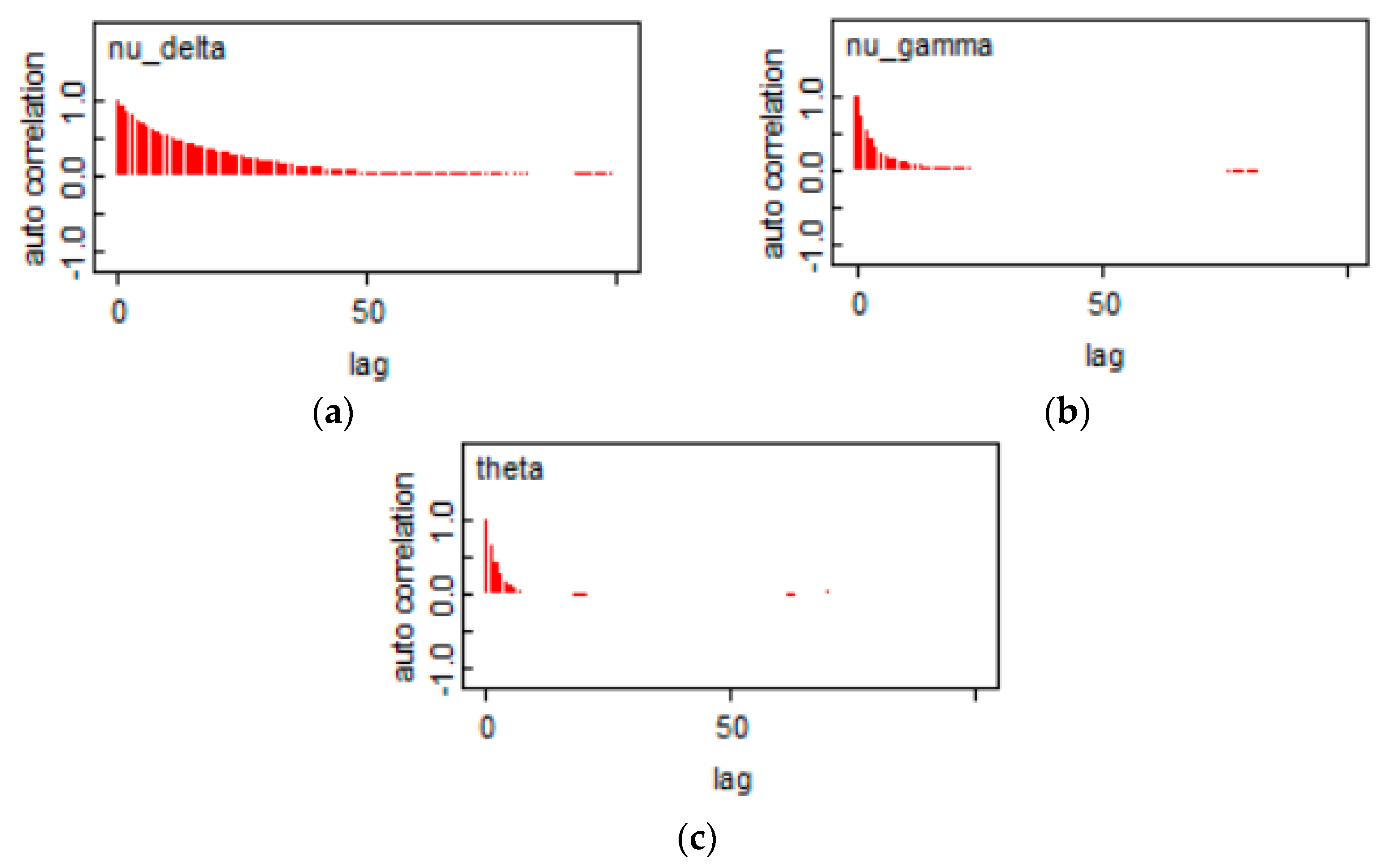
In the MCMC method, convergence assessment is pivotal. Reliance on results from non-convergent MCMC iterations can lead to inaccurate and potentially misleading conclusions. We typically assess convergence using trace plots or autocorrelation function plots. Trace plots juxtapose simulation values of parameters against their iteration counts. A lack of significant irregularities in these plots during the sampling iterations suggests computational convergence. Meanwhile, the autocorrelation function, which evaluates correlations in simulation data sets, also serves as a convergence indicator. When the autocorrelation value nears zero as iterations increase, the algorithm is considered to have achieved convergence. Utilizing OpenBUGS for the MCMC method, the autocorrelation function plot demonstrates satisfactory convergence for all parameters, as shown in Figure 1.
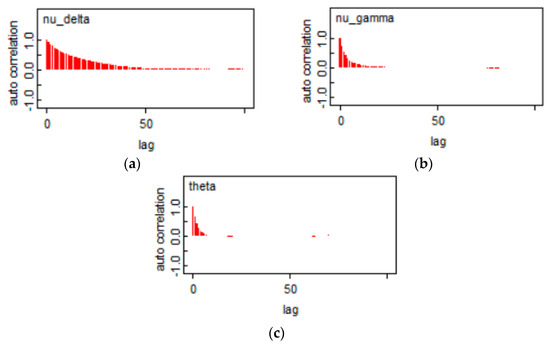
Figure 1.
The autocorrelation functions of parameters. (a) The autocorrelation functions of . (b) The autocorrelation functions of . (c) The autocorrelation functions of .
According to Equation (29), the estimation results of the model parameters can be obtained using the Bayesian computation software OpenBUGS, as shown in Table 1.

Table 1.
Estimation results of model parameters.
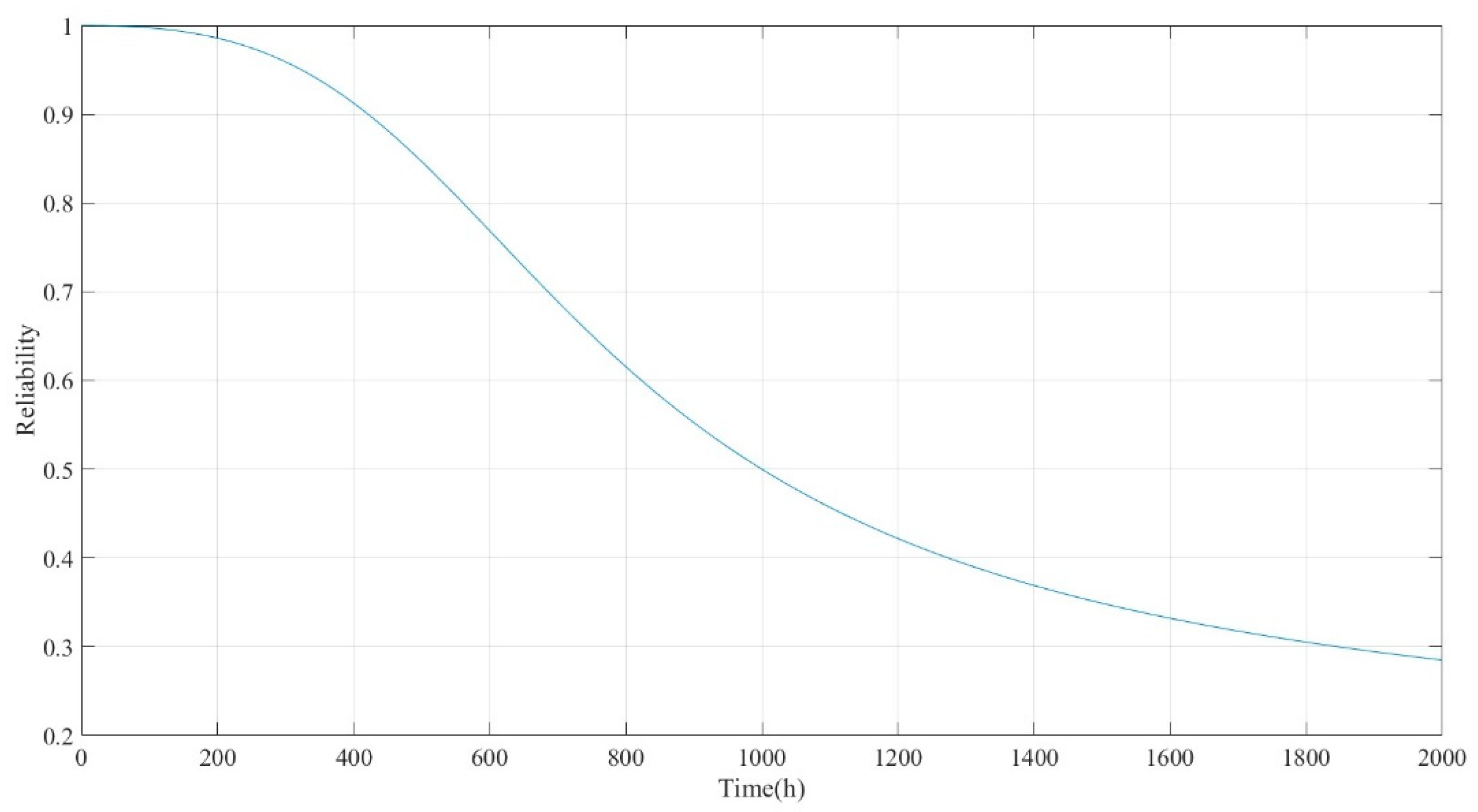
Based on the parameter estimation results shown in Table 1, the reliability assessment results of the spindle system, as illustrated in Figure 2, can be acquired using Equation (31).
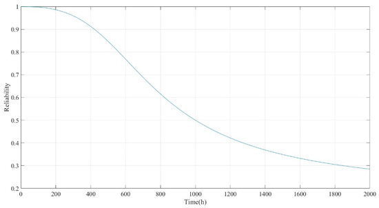
Figure 2.
Reliability of the spindle system.
5. Conclusions
This paper introduces a method for the reliability assessment of industrial equipment through the integration of degradation and failure time data. A holistic framework for reliability analysis is provided by merging these two distinct data types. Employing the Wiener process model, the method captures individual differences in the product degradation process. This dual-pronged approach enhances an understanding of product degradation behaviors and improves predictions of future performance. The methodology addresses both the statistical characteristics of product degradation and variations among products, essential for industrial applications requiring high precision and reliability. This integrated approach enables a more accurate evaluation of equipment reliability over its entire service life, proving valuable for preventive maintenance and risk management.
Potential refinements for the proposed Bayesian-fusion-based methodology could include the integration of more advanced machine learning algorithms to improve the accuracy and efficiency of the model, particularly in handling large datasets. Another area for enhancement is the development of real-time monitoring capabilities, allowing for dynamic updates to reliability assessments as new data become available.
Author Contributions
Methodology, G.-Z.F. and J.G.; Software, X.Z.; Validation, W.L.; Formal analysis, X.Z.; Investigation, J.G.; Writing—original draft, G.-Z.F.; Writing—review & editing, G.-Z.F.; Supervision, G.-Z.F. and W.L. All authors have read and agreed to the published version of the manuscript.
Funding
This research was supported by the Natural Science Foundation of Sichuan, China (grant no. 2023NSFSC856) and National Defense Science and Technology Key Laboratory Stabilization Support.
Data Availability Statement
Data are contained within the article.
Conflicts of Interest
The authors declare no conflict of interest.
References
- Yazdi, M.; Mohammadpour, J.; Li, H.; Huang, H.Z.; Zarei, E.; Pirbalouti, R.G.; Adumene, S. Fault tree analysis improvements: A bibliometric analysis and literature review. Qual. Reliab. Eng. Int. 2023, 39, 1639–1659. [Google Scholar] [CrossRef]
- Li, H.; Guo, J.Y.; Yazdi, M.; Nedjati, A.; Adesina, K.A. Supportive emergency decision-making model towards sustainable development with fuzzy expert system. Neural Comput. Appl. 2021, 33, 15619–15637. [Google Scholar] [CrossRef]
- Li, J.; Zhang, G.; Cabecinhas, D.; Pascoal, A.; Zhang, W. Prescribed performance path following control of USVs via an output-based threshold rule. IEEE Trans. Veh. Technol. 2023, 3338518. [Google Scholar] [CrossRef]
- Nguyen, H.; Sun, X.; Lu, Q.; Zhang, Q.; Li, M. Bayesian heterogeneous degradation performance modeling with an unknown number of sub-populations. Qual. Reliab. Eng. Int. 2023, 39, 2686–2705. [Google Scholar] [CrossRef]
- Li, Y.; Liu, Z.; He, Z.; Tu, L.; Huang, H.Z. Fatigue reliability analysis and assessment of offshore wind turbine blade adhesive bonding under the coupling effects of multiple environmental stresses. Reliab. Eng. Syst. Saf. 2023, 238, 109426. [Google Scholar] [CrossRef]
- Li, H.; Huang, C.G.; Soares, C.G. A real-time inspection and opportunistic maintenance strategies for floating offshore wind turbines. Ocean Eng. 2022, 256, 111433. [Google Scholar] [CrossRef]
- Ye, H.; Li, W.; Lin, S.; Ge, Y.; Lv, Q. A framework for fault detection method selection of oceanographic multi-layer winch fibre rope arrangement. Measurement 2024, 226, 114168. [Google Scholar] [CrossRef]
- Yazdi, M.; Ding, Y.; Adumene, S.; Shafie, P. Progressive system safety and reliability analysis: A sustainable game theory approach. Qual. Reliab. Eng. Int. 2023, 39, 1559–1572. [Google Scholar] [CrossRef]
- Huang, T.; Shao, Z.; Xiahou, T.; Liu, Y. An evidential network approach to reliability assessment by aggregating system-level imprecise knowledge. Qual. Reliab. Eng. Int. 2023, 39, 1863–1877. [Google Scholar] [CrossRef]
- Liu, D.; Ai, S.; Kang, Z.; Sun, L. Fatigue reliability assessment of offshore catenary risers conveying internal slug flow. Qual. Reliab. Eng. Int. 2023, 39, 1994–2010. [Google Scholar] [CrossRef]
- Li, X.Y.; Li, X.; Feng, J.; Li, C.; Xiong, X.; Huang, H.Z. Reliability analysis and optimization of multi-phased spaceflight with backup missions and mixed redundancy strategy. Reliab. Eng. Syst. Saf. 2023, 237, 109373. [Google Scholar] [CrossRef]
- Zhang, Z.; Dong, S.; Li, D.; Liu, P.; Wang, Z. Prediction and Diagnosis of Electric Vehicle Battery Fault Based on Abnormal Voltage: Using Decision Tree Algorithm Theories and Isolated Forest. Processes 2024, 12, 136. [Google Scholar] [CrossRef]
- Li, H.; Soares, C.G.; Huang, H.Z. Reliability analysis of a floating offshore wind turbine using Bayesian Networks. Ocean Eng. 2020, 217, 107827. [Google Scholar] [CrossRef]
- Liu, Z.; Soares, C.G. Sensitivity analysis of the cage volume and mooring forces for a gravity cage subjected to current and waves. Ocean Eng. 2023, 287, 115715. [Google Scholar] [CrossRef]
- Yan, B.; Ma, X.; Huang, G.; Zhao, Y. Two-stage physics-based Wiener process models for online RUL prediction in field vibration data. Mech. Syst. Signal Process. 2021, 152, 107378. [Google Scholar] [CrossRef]
- Huang, C.G.; Zhu, J.; Han, Y.; Peng, W. A novel Bayesian deep dual network with unsupervised domain adaptation for transfer fault prognosis across different machines. IEEE Sens. J. 2021, 22, 7855–7867. [Google Scholar] [CrossRef]
- Wang, X.; Jiang, P.; Guo, B.; Cheng, Z. Real-time reliability evaluation with a general Wiener process-based degradation model. Qual. Reliab. Eng. Int. 2014, 30, 205–220. [Google Scholar] [CrossRef]
- Li, H.; Pan, D.; Chen, C.P. Reliability modeling and life estimation using an expectation maximization based wiener degradation model for momentum wheels. IEEE Trans. Cybern. 2014, 45, 969–977. [Google Scholar]
- Gao, H.; Cui, L.; Kong, D. Reliability analysis for a Wiener degradation process model under changing failure thresholds. Reliab. Eng. Syst. Saf. 2018, 171, 1–8. [Google Scholar] [CrossRef]
- Wang, X.; Balakrishnan, N.; Guo, B. Mis-specification analyses of nonlinear Wiener process-based degradation models. Commun. Stat. Simul. Comput. 2016, 45, 814–832. [Google Scholar] [CrossRef]
- Li, T.; Pei, H.; Pang, Z.; Si, X.; Zheng, J. A sequential Bayesian updated Wiener process model for remaining useful life prediction. IEEE Access 2019, 8, 5471–5480. [Google Scholar] [CrossRef]
- Hu, Y.; Li, H.; Shi, P.; Chai, Z.; Wang, K.; Xie, X.; Chen, Z. A prediction method for the real-time remaining useful life of wind turbine bearings based on the Wiener process. Renew. Energy 2018, 127, 452–460. [Google Scholar] [CrossRef]
- Dai, L.; Guo, J.; Wan, J.L.; Wang, J.; Zan, X. A reliability evaluation model of rolling bearings based on WKN-BiGRU and Wiener process. Reliab. Eng. Syst. Saf. 2022, 225, 108646. [Google Scholar] [CrossRef]
- Liu, D.; Wang, S.; Zhang, C. Reliability estimation from two types of accelerated testing data based on an artificial neural network supported Wiener process. Appl. Math. Comput. 2022, 417, 126757. [Google Scholar] [CrossRef]
- Guan, Q.; Wei, X.; Zhang, H.; Jia, L. Remaining useful life prediction for degradation processes based on the Wiener process considering parameter dependence. Qual. Reliab. Eng. Int. 2023, 3461. [Google Scholar] [CrossRef]
- Shi, J.; Qiao, Y.; Wang, S.; Cui, X.; Liu, D. A reliability estimation method based on two-phase Wiener process with evidential variable using two types of testing data. Qual. Reliab. Eng. Int. 2023, 39, 229–243. [Google Scholar] [CrossRef]
- Lin, W.; Chai, Y.; Fan, L.; Zhang, K. Remaining useful life prediction using nonlinear multi-phase Wiener process and variational Bayesian approach. Reliab. Eng. Syst. Saf. 2023, 242, 109800. [Google Scholar] [CrossRef]
- Zhang, Z.; Zhang, J.; Du, D.; Li, T.; Si, X. A lifetime estimation method for multi-component degrading systems with deteriorating spare parts. Reliab. Eng. Syst. Saf. 2023, 238, 109427. [Google Scholar] [CrossRef]
- Ma, J.; Cai, L.; Liao, G.; Yin, H.; Si, X.; Zhang, P. A multi-phase Wiener process-based degradation model with imperfect maintenance activities. Reliab. Eng. Syst. Saf. 2023, 232, 109075. [Google Scholar] [CrossRef]
- Yan, B.; Wang, H.; Ma, X. Correlation-driven multivariate degradation modeling and RUL prediction based on Wiener process model. Qual. Reliab. Eng. Int. 2023, 39, 3203–3229. [Google Scholar] [CrossRef]
- Yazdi, M.; Khan, F.; Abbassi, R. Operational subsea pipeline assessment affected by multiple defects of microbiologically influenced corrosion. Process Saf. Environ. Prot. 2022, 158, 159–171. [Google Scholar] [CrossRef]
- Li, X.; Zhan, K.; Xiong, X.; Vu, T.Q. A copula-based reliability model for phased mission systems with dependent components PMS with dependent components. Qual. Reliab. Eng. Int. 2023, 39, 1533–1547. [Google Scholar] [CrossRef]
- Wang, Z.; Guo, J.; Wang, J.; Yang, Y.; Dai, L.; Huang, C.G.; Wan, J.L. A deep learning based health indicator construction and fault prognosis with uncertainty quantification for rolling bearings. Meas. Sci. Technol. 2023, 34, 105015. [Google Scholar] [CrossRef]
- Ni, Q.; Ji, J.C.; Halkon, B.; Feng, K.; Nandi, A.K. Physics-Informed Residual Network (PIResNet) for rolling element bearing fault diagnostics. Mech. Syst. Signal Process. 2023, 200, 110544. [Google Scholar] [CrossRef]
- Zhang, M.; Li, D.; Wang, K.; Li, Q.; Ma, Y.; Liu, Z.; Kang, T. An adaptive order-band energy ratio method for the fault diagnosis of planetary gearboxes. Mech. Syst. Signal Process. 2022, 165, 108336. [Google Scholar] [CrossRef]
- Li, H.; Diaz, H.; Soares, C.G. A developed failure mode and effect analysis for floating offshore wind turbine support structures. Renew. Energy 2021, 164, 133–145. [Google Scholar] [CrossRef]
- Yazdi, M.; Zarei, E.; Pirbalouti, R.G.; Li, H. A comprehensive resilience assessment framework for hydrogen energy infrastructure development. Int. J. Hydrogen Energy 2024, 51, 928–947. [Google Scholar] [CrossRef]
- Li, D.; Zhang, M.; Kang, T.; Ma, Y.; Xiang, H.; Yu, S.; Wang, K. Frequency Energy Ratio Cell Based Operational Security Domain Analysis of Planetary Gearbox. IEEE Trans. Reliab. 2022, 72, 49–60. [Google Scholar] [CrossRef]
- Li, H.; Díaz, H.; Soares, C.G. A failure analysis of floating offshore wind turbines using AHP-FMEA methodology. Ocean Eng. 2021, 234, 109261. [Google Scholar] [CrossRef]
- Mi, J.; Lu, N.; Li, Y.F.; Huang, H.Z.; Bai, L. An evidential network-based hierarchical method for system reliability analysis with common cause failures and mixed uncertainties. Reliab. Eng. Syst. Saf. 2022, 220, 108295. [Google Scholar] [CrossRef]
- Li, F.; Yang, S.; Yang, Z.; Shi, H.; Zeng, J.; Ye, Y. A novel vertical elastic vibration reduction for railway vehicle carbody based on minimum generalized force principle. Mech. Syst. Signal Process. 2023, 189, 110035. [Google Scholar] [CrossRef]
- Jiang, G.; Duan, Z.; Zhao, Q.; Li, D.; Luan, Y. Remaining useful life prediction of rolling bearings based on TCN-MSA. Meas. Sci. Technol. 2023, 35, 025125. [Google Scholar] [CrossRef]
- Wang, X. Wiener processes with random effects for degradation data. J. Multivar. Anal. 2010, 101, 340–351. [Google Scholar] [CrossRef]
- Hao, H.; Su, C. A Bayesian framework for reliability assessment via wiener process and MCMC. Math. Probl. Eng. 2014, 2014, 486368. [Google Scholar] [CrossRef]
- Pan, D.; Liu, J.B.; Huang, F.; Cao, J.; Alsaedi, A. A Wiener process model with truncated normal distribution for reliability analysis. Appl. Math. Model. 2017, 50, 333–346. [Google Scholar] [CrossRef]
- Zhai, Q.; Chen, P.; Hong, L.; Shen, L. A random-effects Wiener degradation model based on accelerated failure time. Reliab. Eng. Syst. Saf. 2018, 180, 94–103. [Google Scholar] [CrossRef]
- Wang, X.; Balakrishnan, N.; Guo, B. Residual life estimation based on a generalized Wiener process with skew-normal random effects. Commun. Stat. Simul. Comput. 2016, 45, 2158–2181. [Google Scholar] [CrossRef]
- Duan, F.; Wang, G.; Wei, W.; Jiang, M. Remaining useful life evaluation for accelerated Wiener degradation process model with mixed random effects and measurement errors. Qual. Reliab. Eng. Int. 2023, 39, 1334–1351. [Google Scholar] [CrossRef]
- Wang, X.; Wang, B.X.; Wu, W.; Hong, Y. Reliability analysis for accelerated degradation data based on the Wiener process with random effects. Qual. Reliab. Eng. Int. 2020, 36, 1969–1981. [Google Scholar] [CrossRef]
- Zheng, H.; Yang, J.; Xu, H.; Zhao, Y. Reliability acceptance sampling plan for degraded products subject to Wiener process with unit heterogeneity. Reliab. Eng. Syst. Saf. 2023, 229, 108877. [Google Scholar] [CrossRef]
- Yan, B.; Wang, H.; Ma, X. Modeling left-truncated degradation data using random drift-diffusion Wiener processes. Qual. Technol. Quant. Manag. 2023, 21, 2187011. [Google Scholar] [CrossRef]
- Tang, S.; Wang, F.; Sun, X.; Xu, X.; Yu, C.; Si, X. Unbiased parameters estimation and mis-specification analysis of Wiener process-based degradation model with random effects. Appl. Math. Model. 2022, 109, 134–160. [Google Scholar] [CrossRef]
- Hou, Y.; Du, Y.; Peng, Y.; Liu, D. An improved random effects Wiener process accelerated degradation test model for lithium-ion battery. IEEE Trans. Instrum. Meas. 2021, 70, 3091457. [Google Scholar] [CrossRef]
- Wang, L.; Zhang, Y.; Bao, Y.; Ma, T. Numerical study of transient flow characteristics of gas-liquid two-phase flow in inclined upward tube under periodic vibration. Ocean Eng. 2023, 282, 115024. [Google Scholar] [CrossRef]
- Zeng, Y.; Huang, T.; Zhang, T.; Huang, H.Z. System Level Performance Degradation Prediction for Power Converters Based on SSA Elman NN and Empirical Knowledge. IEEE Trans. Ind. Inform. 2024, 20, 1240–1250. [Google Scholar] [CrossRef]
- Guo, J.; Zan, X.; Wang, L.; Lei, L.; Ou, C.; Bai, S. A random forest regression with Bayesian optimization-based method for fatigue strength prediction of ferrous alloys. Eng. Fract. Mech. 2023, 293, 109714. [Google Scholar] [CrossRef]
- Yazdi, M.; Khan, F.; Abbassi, R. A dynamic model for microbiologically influenced corrosion (MIC) integrity risk management of subsea pipelines. Ocean Eng. 2023, 269, 113515. [Google Scholar] [CrossRef]
- Yazdi, M.; Moradi, R.; Pirbalouti, R.G.; Zarei, E.; Li, H. Enabling Safe and Sustainable Hydrogen Mobility: Circular Economy-Driven Management of Hydrogen Vehicle Safety. Processes 2023, 11, 2730. [Google Scholar] [CrossRef]
- Bai, S.; Huang, T.; Li, Y.F.; Lu, N.; Huang, H.Z. A probabilistic fatigue life prediction method under random combined high and low cycle fatigue load history. Reliab. Eng. Syst. Saf. 2023, 238, 109452. [Google Scholar] [CrossRef]
- Chen, H.; He, X.; Yang, H.; Wu, Y.; Qing, L.; Sheriff, R.E. Self-supervised cycle-consistent learning for scale-arbitrary real-world single image super-resolution. Expert Syst. Appl. 2023, 212, 118657. [Google Scholar] [CrossRef]
- Zhu, R.; Peng, W.; Wang, D.; Huang, C.G. Bayesian transfer learning with active querying for intelligent cross-machine fault prognosis under limited data. Mech. Syst. Signal Process. 2023, 183, 109628. [Google Scholar] [CrossRef]
- Guo, J.; Wan, J.L.; Yang, Y.; Dai, L.; Tang, A.; Huang, B.; Zhang, F.; Li, H. A deep feature learning method for remaining useful life prediction of drilling pumps. Energy 2023, 282, 128442. [Google Scholar] [CrossRef]
- Li, H.; Teixeira, A.P.; Soares, C.G. A two-stage Failure Mode and Effect Analysis of offshore wind turbines. Renew. Energy 2020, 162, 1438–1461. [Google Scholar] [CrossRef]
- Pan, R. A Bayes approach to reliability prediction utilizing data from accelerated life tests and field failure observations. Qual. Reliab. Eng. Int. 2009, 25, 229–240. [Google Scholar] [CrossRef]
- Wang, L.; Pan, R.; Li, X.; Jiang, T. A Bayesian reliability evaluation method with integrated accelerated degradation testing and field information. Reliab. Eng. Syst. Saf. 2013, 112, 38–47. [Google Scholar] [CrossRef]
- Zhao, Q.; Jia, X.; Cheng, Z.; Guo, B. Bayesian estimation of residual life for Weibull-distributed components of on-orbit satellites based on multi-source information fusion. Appl. Sci. 2019, 9, 3017. [Google Scholar] [CrossRef]
- Wang, L.; Pan, R.; Wang, X.; Fan, W.; Xuan, J. A Bayesian reliability evaluation method with different types of data from multiple sources. Reliab. Eng. Syst. Saf. 2017, 167, 128–135. [Google Scholar] [CrossRef]
- Chen, R.; Zhang, C.; Wang, S.; Hong, L. Bivariate-Dependent Reliability Estimation Model Based on Inverse Gaussian Processes and Copulas Fusing Multisource Information. Aerospace 2022, 9, 392. [Google Scholar] [CrossRef]
- Guo, J.; Li, Y.F.; Peng, W.; Huang, H.Z. Bayesian information fusion method for reliability analysis with failure-time data and degradation data. Qual. Reliab. Eng. Int. 2022, 38, 1944–1956. [Google Scholar] [CrossRef]
- Chen, W.B.; Li, X.Y.; Kang, R. Integration for degradation analysis with multi-source ADT datasets considering dataset discrepancies and epistemic uncertainties. Reliab. Eng. Syst. Saf. 2022, 222, 108430. [Google Scholar] [CrossRef]
- Kang, W.; Tian, Y.; Xu, H.; Wang, D.; Zheng, H.; Zhang, M.; Mu, H. Reliability analysis based on the Wiener process integrated with historical degradation data. Qual. Reliab. Eng. Int. 2023, 39, 1376–1395. [Google Scholar] [CrossRef]
- Li, H.; Soares, C.G. Assessment of failure rates and reliability of floating offshore wind turbines. Reliab. Eng. Syst. Saf. 2022, 228, 108777. [Google Scholar] [CrossRef]
- Huang, P.; Li, H.; Gu, Y.; Qiu, G.; Ding, Y. Experimental tolerance design of robot manipulators accounting for positioning accuracy reliability. Qual. Reliab. Eng. Int. 2023, 39, 1573–1587. [Google Scholar] [CrossRef]
- Wang, J.; Guo, J.; Wang, L.; Yang, Y.; Wang, Z.; Wang, R. A hybrid intelligent rolling bearing fault diagnosis method combining WKN-BiLSTM and attention mechanism. Meas. Sci. Technol. 2023, 34, 085106. [Google Scholar] [CrossRef]
- Wang, L.; Chen, J.; Ma, T.; Ma, R.; Bao, Y.; Fan, Z. Numerical study of leakage characteristics of hydrogen-blended natural gas in buried pipelines. Int. J. Hydrog. Energy 2023, 49, 1166–1179. [Google Scholar] [CrossRef]
- Li, H.; Peng, W.; Huang, C.G.; Guedes Soares, C. Failure rate assessment for onshore and floating offshore wind turbines. J. Mar. Sci. Eng. 2022, 10, 1965. [Google Scholar] [CrossRef]
- Niazi, S.G.; Huang, T.; Zhou, H.; Bai, S.; Huang, H.Z. Multi-scale time series analysis using TT-ConvLSTM technique for bearing remaining useful life prediction. Mech. Syst. Signal Process. 2024, 206, 110888. [Google Scholar] [CrossRef]
- Yazdi, M.; Golilarz, N.A.; Nedjati, A.; Adesina, K.A. An improved lasso regression model for evaluating the efficiency of intervention actions in a system reliability analysis. Neural Comput. Appl. 2021, 33, 7913–7928. [Google Scholar] [CrossRef]
- Jiang, G.J.; Yang, J.S.; Cheng, T.C.; Sun, H.H. Remaining useful life prediction of rolling bearings based on Bayesian neural network and uncertainty quantification. Qual. Reliab. Eng. Int. 2023, 39, 1756–1774. [Google Scholar] [CrossRef]
- Li, Y.F.; Huang, H.Z.; Mi, J.; Peng, W.; Han, X. Reliability analysis of multi-state systems with common cause failures based on Bayesian network and fuzzy probability. Ann. Oper. Res. 2022, 311, 195–209. [Google Scholar] [CrossRef]
- Guo, J.; Wang, J.; Wang, Z.; Gong, Y.; Qi, J.; Wang, G.; Tang, C. A CNN-BiLSTM-Bootstrap integrated method for remaining useful life prediction of rolling bearings. Qual. Reliab. Eng. Int. 2023, 39, 1796–1813. [Google Scholar] [CrossRef]
- Li, Y.F.; Mi, J.; Liu, Y.U.; Yang, Y.J.; Huang, H.Z. Dynamic fault tree analysis based on continuous-time Bayesian networks under fuzzy numbers. Proc. Inst. Mech. Eng. Part O J. Risk Reliab. 2015, 229, 530–541. [Google Scholar] [CrossRef]
- Chen, H.; He, X.; Yang, H.; Feng, J.; Teng, Q. A two-stage deep generative adversarial quality enhancement network for real-world 3D CT images. Expert Syst. Appl. 2022, 193, 116440. [Google Scholar] [CrossRef]
- Yang, Y.J.; Liu, G.H.; Yu, P.; Huang, C.; Li, L. Dynamic response and safety analysis of polyethylene pipeline under rockfall conditions. Qual. Reliab. Eng. Int. 2023, 39, 2044–2068. [Google Scholar] [CrossRef]
- Yazdi, M.; Khan, F.; Abbassi, R. Microbiologically influenced corrosion (MIC) management using Bayesian inference. Ocean Eng. 2021, 226, 108852. [Google Scholar] [CrossRef]
- Cai, W.; Wu, X.; Chi, M.; Huang, H.Z. High-order wheel polygonal wear growth and mitigation: A parametric study. Mech. Syst. Signal Process. 2023, 186, 109917. [Google Scholar] [CrossRef]
- Zeng, Y.; Huang, T.; Li, Y.F.; Huang, H.Z. Reliability modeling for power converter in satellite considering periodic phased mission. Reliab. Eng. Syst. Saf. 2023, 232, 109039. [Google Scholar] [CrossRef]
- Xu, Z.; Bashir, M.; Liu, Q.; Miao, Z.; Wang, X.; Wang, J.; Ekere, N. A novel health indicator for intelligent prediction of rolling bearing remaining useful life based on unsupervised learning model. Comput. Ind. Eng. 2023, 176, 108999. [Google Scholar] [CrossRef]
Disclaimer/Publisher’s Note: The statements, opinions and data contained in all publications are solely those of the individual author(s) and contributor(s) and not of MDPI and/or the editor(s). MDPI and/or the editor(s) disclaim responsibility for any injury to people or property resulting from any ideas, methods, instructions or products referred to in the content. |
© 2024 by the authors. Licensee MDPI, Basel, Switzerland. This article is an open access article distributed under the terms and conditions of the Creative Commons Attribution (CC BY) license (https://creativecommons.org/licenses/by/4.0/).