Quality of Mixedness Using Information Entropy in a Counter-Current Three-Phase Bubble Column

Abstract

Knowledge of mixing phenomena is of great value in the mineral and other chemical and biochemical industries. This work aims to analyze the quality of mixedness (QM), the intrinsic mass transfer (MT) number, and the MT efficiency based on information entropy theory in the counter-current microstructured slurry bubble column. A thorough analysis is conducted to assess the effects of particle loading, gas and slurry velocity, and axial variation on the QM. The range of gas velocity, slurry velocity, particle size, and particle loading was 0.011–0.075 m/s, 0.018–0.058 m/s, 242.72–408.31 μm, and 15.54–88.94 kg/m³, respectively. QM is a time-dependent parameter, and the concept of contact time has been used for scale-up purposes. The maximum QM was achieved at dimensionless times of 0.40 × 10⁻³, 0.15 × 10⁻³, and 0.85 × 10⁻³ for the maximum superficial gas velocity, particle loading, and axial height, respectively. The gas velocity positively influenced both the intrinsic MT number and its efficiency. In contrast, the slurry velocity and particle loading had a negative effect. The present theoretical analysis will pave the path for industrial process intensification in counter-current flow systems.

1. Introduction

A slurry bubble column (SBC) is a three-phase contactor and is widely used for its simple construction, low operating cost, low maintenance, excellent mass transfer (MT) and heat transfer, high slurry content, low energy consumption, owing to the inlet gas-induced mixing, and high selectivity [1,2]. SBCs are used in the petrochemical, biochemical, and mineral industries. Depending on the requirement, these columns are typically operated in one of three modes, namely semi-batch, co-current, and counter-current. Hydrodynamic studies such as gas holdup, bubble size distribution, frictional pressure drop, and mixing characteristics are some of the important design parameters for scale-up purposes and for improving the efficiency of the process in the SBC. Mixing characteristics are one of the most important design parameters for defining the performance of the SBC. Several researchers have quantified mixing experimentally; however, the enunciation of mixing in terms of the quality of mixedness (QM) applying the information entropy (IE) theory in counter-current systems still remains unexplored. Therefore, the current study mainly focuses on the theoretical analysis of the mixing quality in the counter-current SBC.

Studying hydrodynamic characteristics in the two-phase system is easier than in the three-phase system. Also, adding the third phase as a solid particle complicates the hydrodynamic behavior in terms of control, ease of operation, and low interfacial area of contact between the phases. A large number of mixing studies have been conducted by researchers, mainly in the two-phase semi-batch [3,4], co-current up flow [5,6], and counter-current mode [7]. Some studies in the three-phase semi-batch, co-current up flow [8], and counter-current [9] systems were also performed. Studies conducted in the counter-current three-phase system are relatively scarce compared to the two-phase semi-batch, co-current up, and downflow systems. Therefore, understanding the mixing behavior in the counter-current three-phase system is of utmost importance.

Backmixing is prevalent in the cylindrical column [10]. It adversely affects selectivity and conversion [11,12], especially when the intermediate is the desired product [13]. Some authors have reported using internals (i.e., sieve plates, packing, channels, etc.) to reduce global liquid circulation [14,15,16]. However, other researchers have reported that arranging internals such as vertical tubes can accelerate liquid phase circulation [17,18]. A rectangular column with a small depth can also be helpful in reducing the amount of backmixing in the SBC. Peclet number is said to characterize the intensity of the backmixing [19]. The lower the Peclet number, the higher the backmixing. The degree of axial mixing increases with the diameter of the column [20,21,22]. Several two- and three-phase studies have reported that the axial mixing increases as the gas inlet increases, regardless of the mode of operation [4,20,21,23]. However, the influence of the continuous phase velocity on axial mixing depends on the operating mode. Axial mixing increases as the liquid velocity increases in both co-current and counter-current modes (in the two-phase system) [20], has a negligible influence on the inlet slurry velocity in the co-current operation (in the three-phase) [23], and increases with the slurry velocity [24]. Notably, the axial mixing reported in the counter-current mode was higher compared to the co-current mode [20]. The hydrodynamic characteristics of the three-phase system are entirely different from those of the two-phase system. The addition of the third phase as a solid to the liquid and its concentration and size significantly influence the behavior of the axial mixing. Some studies suggest that the addition of solid particles to the liquid reduces axial mixing [24,25], whereas other authors have reported a negligible effect [23]. An approximately 40% decrease in axial mixing has been reported by Ityokumbul et al. [25] in the presence of solid particles. The size of the particles in the three-phase system influences the intensity of axial mixing. The effect of particle size on axial mixing is not clear. In the three-phase co-current operation, axial mixing was independent of the particle size [23]. Some researchers have quantified the axial and radial mixing [1,26], indicating that the value of radial mixing was 1/10 [1] and 1% [26] of axial mixing.

The axial mixing of the slurry phase can be quantified by analyzing the QM behavior in the SBC. Based on the IE theory, Nedeltchev et al. [27] introduced the fundamental concept of “quality of mixedness” (QM). The IE theory has been used in the past for the identification of flow regimes in SBC [28]. A comprehensive literature review reveals that there is no information available on the QM, the intrinsic MT number, and the overall MT efficiency based on the IE theory in the counter-current microstructured SBC. The effects of gas and slurry flow rates, particle loading, and axial variation are studied. In the present work, experimental data from Prakash et al. [24] are used to enunciate the QM by applying the IE theory proposed by Nedeltchev et al. [27]. Understanding the QM, intrinsic MT number, and overall MT efficiency is crucial for both scaling up the process and enhancing its efficiency in counter-current SBCs. This knowledge is essential for optimizing conditions and ensuring effective MT in the system, contributing to improved performance and scalability.

2. Experimentation

The schematic diagram of the experimental setup is shown in Figure 1. In-depth details of the experimentation are given elsewhere [24]. The experimental setup consists of the microstructured column (length: 0.63 m, width: 0.19 m, and depth: 0.03 m) and other accessories such as the gas rotameter, the electromagnetic flow meter, the solenoid valve, the stirrer, the slurry pump, the slurry tank, the air compressor, the stainless steel porous plate cylindrical sparger (average pore diameter of about 20 µm), the control valves, and the needle valve. The height of the gas–slurry dispersion in the column was kept at a constant level of 0.49 m for all the experiments. Air, water, and coal particles were used as the gas, liquid, and solid phases. The experiment was carried out in the range of inlet gas velocities from 0.011 to 0.075 m/s, the inlet slurry velocities range from 0.018 to 0.058 m/s, the particle loading range from 15.54 to 88.94 kg/m³, and the average particle size range from 63.01 to 408.31 μm. The inlet gas and slurry velocity were calculated by dividing the volumetric flow rate by the cross-sectional area of the column. Slurry consists of coal particles and water. All the experiments were conducted with the Methyl Isobutyl Carbinol surfactant. One molar of 10 mL of potassium chloride (KCl) was used as a tracer. A high-pressure spring-loaded syringe introduced the tracer to the inlet slurry. The conductivity probes determined the mixing characteristics by online measuring the tracer concentration over time. Mixing was studied at six different positions in the axial and transverse directions. The aspect ratio (AR) in the axial direction was as follows: 0.89 (probe 1), 1.63 (probe 2), 2.11 (probe 3), and 2.11 (probe 4), and in the transverse direction, 0.53 (probe 2), 0.74 (probe 5), and 1.0 (probe 6). The particle shape, the particle size distribution, the physical properties of the slurry, and the conductivity meter calibration table are provided in the previous article [24].

3. Theoretical Background

3.1. Information Entropy (IE) Theory

Mixing characteristics in the SBC reactor can also be analyzed by means of the IE theory. This theory contributes to the idea of the QM, which helps to determine the efficiency of SBCs. The IE method measures the extent of the uncertainty related to an arbitrary variable [27]. The cumulative distribution function defines the randomness of a variable and estimates the probability distribution of a control volume. A probability distribution can completely describe the probability distribution related to a real-valued random variable (X). For each real number x, the cumulative distribution function of X is expressed as

$$x\to F_{\mathrm{x}}\left(x\right)=P(X\le x)$$

(1)

The IE of a discrete random variable $X$ can be taken as a range of values, such as $\left\{x_1,x_2..............x_{\mathrm{n}}\right\}$ and can be expressed as

$$(X)=E(I(X))=-{\sum }_{i=1}^n{P}_{\mathrm{i}}\left(x_{\mathrm{i}}\right)\log (x_{\mathrm{i}})$$

(2)

where $P\left(x_{\mathrm{i}}\right)$ denotes the probability of a tracer in a column and $I\left(X\right)$ indicates the amount of information.

The IE is related to the average amount of information conveyed by an event when considering all possible outcomes expressed in terms of probabilities. It measures the expected (i.e., average) amount of information obtained by identifying the outcome of a random trial. The IE could be interpreted as a measure of how informative the average outcome of an event is. The IE definition is based on the probability distribution when observing a specific event. In the case of a highly likely event, very little information is obtained, and vice versa. Uniform probability yields maximum uncertainty and, therefore, maximum IE. When the IE is zero bits, then there is no uncertainty at all. The IE of a system can also be interpreted as the amount of “missing” information needed to determine a microstate, provided that the macrostate is known.

The IE is analogous to the entropy in statistical thermodynamics. The IE definition is much more straightforward than the definitions of Kolmogorov entropy, Shannon entropy, Gibbs entropy, thermodynamic entropy, etc.

3.2. Application of IE Theory in a Counter-Current SBC

The SBC was symmetrically divided into layers of semi-rectangular shells with small volumes to implement the IE theory. The tracer concentration needs to be determined in each semi-rectangular shell of a small volume. The total volume of the column was discretized into 1000 parts. The probability of the appearance of the tracer $\left(P_{\mathrm{i}}\right(t\left)\right)$ in a given semi-rectangular shell could then be derived from experimentally determined concentration values $\left(C_{\mathrm{i}}\right(t\left)\right)$ of the tracer, as follows:

$$P_{\mathrm{i}}(t)=\frac{C_{\mathrm{i}}\left(t\right)V_{\mathrm{i}}}{{\sum }_{i=1}^n{C}_{\mathrm{i}}\left(t\right)V_{\mathrm{i}}}$$

(3)

where V_i denotes the volume of semi-rectangular shells of a small volume. This probability calculation allows for a quantitative understanding of the tracer distribution within the various small volumes, forming the basis for subsequent analysis using IE theory. The amount of information I(X) can be evaluated as

$$I_{\mathrm{i}}\left(t\right)=-\mathit{log}(P_{\mathrm{i}}\left(t\right))$$

(4)

Therefore, the IE is represented as

$$H(t)=\sum _{i=1}^n{P}_{\mathrm{i}}\left(t\right)(-\mathit{log}(P_{\mathrm{i}}))$$

(5)

The minimum value of entropy $(H_{\mathrm{m}\mathrm{i}\mathrm{n}}$) is given as

$$H_{\mathrm{m}\mathrm{i}\mathrm{n}}=0$$

(6)

The maximum value of entropy $\left(H_{\mathrm{m}\mathrm{a}\mathrm{x}}\right)$ is represented by

$${H_{\mathrm{m}\mathrm{a}\mathrm{x}}=\frac{V_{\mathrm{i}}}{{\sum }_{i=1}^n{V}_{\mathrm{i}}}\mathit{log}\left(\frac{V_{\mathrm{i}}}{{\sum }_{i=1}^n{V}_{\mathrm{i}}}\right)}_{\mathrm{m}\mathrm{a}\mathrm{x}}$$

(7)

The QM index measures the extent of the asymptotic approach to the state of equilibrium. It can be defined as the degree to which the concentration distribution within the slurry column tends toward uniformity or homogeneity. This measure of mixedness is indicative of how effectively the different components in the system, such as the gas, liquid, and solid phases, are mixed and distributed throughout the column, ultimately influencing the overall performance and efficiency of the counter-current SBC.

$$M(t)=\frac{H\left(t\right)-H_{\mathrm{m}\mathrm{i}\mathrm{n}}}{H_{\mathrm{m}\mathrm{a}\mathrm{x}}}$$

(8)

The QM value $M\left(t\right)$ varies with time (t). The $M\left(t\right)$ values are in the range of $0<M\left(t\right)<1$. The following relationship can express the variation in $M\left(t\right)$ over time:

$$M(t)=\frac{H\left(t\right)-H_{\mathrm{m}\mathrm{i}\mathrm{n}}}{H_{\mathrm{m}\mathrm{a}\mathrm{x}}=f\left(T_{\mathrm{c}}\right)}$$

(9)

where $T_{\mathrm{c}}$ is the ratio of the time $\left(t\right)$ and the average contact time $\left(t_{\mathrm{c}}\right)$ between the bubble and the slurry. The contact time serves as a measure of the duration during which micro eddies reside, playing a crucial role in facilitating MT within the liquid film at the interface between the bubble and the liquid. The dynamics of micro-scale eddies behind the bubbles dictate the control of the surface area at the bubble–liquid interface. The following equation determines the average contact time:

$$t_{\mathrm{c}}=\frac{4E_{\mathrm{z}}}{\pi k_{\mathrm{s}\mathrm{l}}^2}$$

(10)

where $k_{\mathrm{s}\mathrm{l}}$ is the slurry phase MT coefficient and $E_{\mathrm{z}}$ is the axial (longitudinal) mixing coefficient, which can be estimated using the following Equation (11) [24]:

$$\frac{E_{\mathrm{z}}}{u_{\mathrm{g}}z}=0.035{\left(\frac{g{d}_{\mathrm{c}}}{u_{\mathrm{g}}^2}\right)}^{0.380}{\left(\frac{{\rho }_{\mathrm{s}\mathrm{l}}{u}_{\mathrm{l}}^2{d}_{\mathrm{p}}}{{\sigma }_{\mathrm{s}\mathrm{l}}}\right)}^{0.424}{\left(\frac{z}{d_{\mathrm{p}}}\right)}^{0.341}$$

(11)

The value of k_sl is obtained as

$$k_{\mathrm{s}\mathrm{l}}=\frac{k_{\mathrm{s}\mathrm{l}}{ad}_{32}}{6{\alpha }_{\mathrm{g}}}$$

(12)

where ${\alpha }_{\mathrm{g}}$ and $d_{32}$ indicate the volume fraction of gas and the Sauter-mean bubble diameter. In the case of a spherical bubble, the surface area $\left(s_{\mathrm{b}}\right)$ can be calculated as $\pi d_{32}^2$. In the case of an ellipsoidal bubble, the equivalent diameter was measured using the major and minor axes of the bubble [29]. The ${\alpha }_{\mathrm{g}}$ was estimated using the phase isolation technique, which can be estimated by using Equation (13) [30]:

$${\alpha }_{\mathrm{g}}=7.75{\left(\frac{g{d}_{\mathrm{c}}}{u_{\mathrm{g}}^2}\right)}^{-0.639}{\left(\frac{d_{\mathrm{p}}{\rho }_{\mathrm{s}\mathrm{l}}{u}_{\mathrm{l}}^2}{{\sigma }_{\mathrm{s}\mathrm{l}}}\right)}^{0.078}$$

(13)

The bubble size was measured using the photography technique, and the Sauter mean diameter $\left(d_{32}\right)$ was calculated using the following Equation (14), which is expressed as

$$\frac{d_{32}}{d_{\mathrm{c}}}=6\times 10^{-2}{\left(\frac{{\rho }_{\mathrm{s}\mathrm{l}}{u}_{\mathrm{l}}^2{d}_{\mathrm{c}}}{{\sigma }_{\mathrm{s}\mathrm{l}}}\right)}^{-0.018}{\left(\frac{g{d}_{\mathrm{p}}}{u_{\mathrm{g}}^2}\right)}^{-0.124}(1-w_{\mathrm{s}}{)}^{-4.963}$$

(14)

The surface area of the ellipsoidal bubble can be determined using the Fan and Tsuchiya [31] equation:

$$s_{\mathrm{b}}=\pi \left[\frac{l_{\mathrm{m}\mathrm{a}\mathrm{x}}^2}{2}+\frac{l_{\mathrm{m}\mathrm{i}\mathrm{n}}^2}{4\phi }\mathit{ln}\left(\frac{1+\phi }{1-\phi }\right)\right]$$

(15)

where $\phi$ is the aspect ratio and can be determined as

$$\phi =\sqrt{1-\frac{l_{\mathrm{m}\mathrm{i}\mathrm{n}}^2}{l_{\mathrm{m}\mathrm{a}\mathrm{x}}^2}}$$

(16)

The volume of the ellipsoidal bubble $\left(v_{\mathrm{b}}\right)$ is estimated as

$$v_{\mathrm{b}}=\frac{\pi }{6}{l}_{\mathrm{m}\mathrm{a}\mathrm{x}}^2{l}_{\mathrm{m}\mathrm{i}\mathrm{n}}^2$$

(17)

The bubble rise velocity $\left(u_{\mathrm{b}}\right)$ in the three-phase system is calculated by Clift et al. [32]

$$u_{\mathrm{b}}={\left[\frac{2.14{\sigma }_{\mathrm{s}\mathrm{l}}}{{\rho }_{\mathrm{s}\mathrm{l}}{d}_{32}}+0.505g{d}_{32}\right]}^{0.5}$$

(18)

The rate of surface formation $\left(r_{\mathrm{s}}\right)$ of the ellipsoidal bubble is estimated as

$$r_{\mathrm{s}}=u_{\mathrm{b}}{\left[\frac{3}{8}\left(l_{\mathrm{m}\mathrm{a}\mathrm{x}}^2+l_{\mathrm{m}\mathrm{i}\mathrm{n}}^2\right)+\frac{l_{\mathrm{m}\mathrm{a}\mathrm{x}}^2{l}_{\mathrm{m}\mathrm{i}\mathrm{n}}^2}{4}\right]}^{0.5}$$

(19)

The availability of the number of bubbles $\left(n_{\mathrm{b}}\right)$ in the gas–slurry dispersion height is estimated as

$$n_{\mathrm{b}}={\upsilon }_{\mathrm{b}}\frac{h_{\mathrm{m}}}{u_{\mathrm{b}}}$$

(20)

where $\left({\upsilon }_{\mathrm{b}}\right)$ and $\left(h_{\mathrm{m}}\right)$ denote the frequency of bubble formation and the height of the gas–slurry dispersion from the base of the column, respectively. The frequency of bubble formation is estimated as

$${\upsilon }_{\mathrm{b}}=\frac{u_{\mathrm{g}}{A}_{\mathrm{c}}}{v_{\mathrm{b}}}$$

(21)

According to Nedeltchev et al. [33], the correction factor $\left(f_{\mathrm{c}}\right)$ as a function of the Eötvös number $\left(Eo\right)$ [33] can be represented by

$$f_{\mathrm{c}}=0.211E{o}^{0.63}$$

(22)

The correction factor $\left(f_{\mathrm{c}}\right)$ was applied for the correction of the Eo, which was used for the correct measurement of the volumetric MT coefficient (Equation (24)). The correction factor was applied in MT calculations to account for non-ideal conditions in real-world systems. The volumetric MT coefficient $\left(k_{\mathrm{s}\mathrm{l}}a\right)$ is a measure of the efficiency of MT between phases (gas and slurry). The correction factor accounts for non-ideal conditions, the gas–liquid contact area, the temperature and pressure, the liquid properties, and the agitation and mixing.

The Eo can be defined as

$$Eo=\frac{g\left({\rho }_{\mathrm{s}\mathrm{l}}-{\rho }_{\mathrm{g}}\right)d_{32}^2}{{\sigma }_{\mathrm{s}\mathrm{l}}}$$

(23)

The volumetric slurry-side MT coefficient $\left(k_{\mathrm{s}\mathrm{l}}a\right)$ is defined as

$$k_{\mathrm{s}\mathrm{l}}a=f_{\mathrm{c}}\frac{{\upsilon }_{\mathrm{b}}{s}_{\mathrm{b}}}{A_{\mathrm{c}}{u}_{\mathrm{b}}}\sqrt{\frac{4D_{\mathrm{l}}{r}_{\mathrm{s}}}{\pi s_{\mathrm{b}}}}$$

(24)

Using Equations (10)–(24), finally, the QM equation (Equation (9)) is represented as a function of the intrinsic MT number $\left(M_i\right)$ and the Sherwood number $\left(Sh\right)$.

$$M(t)=\frac{H\left(t\right)-H_{\mathrm{m}\mathrm{i}\mathrm{n}}}{H_{\mathrm{m}\mathrm{a}\mathrm{x}}=f\left(T_{\mathrm{c}}\right)=f(M_{\mathrm{i}},Sh)}$$

(25)

The intrinsic MT number indicates the effective MT from the gas phase to the slurry phase during a given contact time and can be represented as

$$M_{\mathrm{i}}=\frac{k_{\mathrm{s}\mathrm{l}}at}{{\alpha }_{\mathrm{g}}}$$

(26)

4. Results and Discussions

4.1. Enunciation of QM Using the IE Theory

In this section, the QM parameter based on the IE theory is enunciated for a three-phase counter-current BC operated under different experimental conditions. The QM is a measure of how well the tracer is distributed throughout the slurry column. The QM has been investigated on the basis of experimental data from Prakash et al. [24] and the proposed model [33]. The QM profile as a function of time is shown in Figure 2. It is observed that the QM increases linearly with time and reaches the maximum value of 1. This implies that the dimensionless QM is a time-dependent quantity.

When scale-up is considered, it is suitable to investigate the behavior of the QM as a function of dimensionless time. For this purpose, dimensionless time is taken as t/t_c. The contact time $\left(t_{\mathrm{c}}\right)$ is calculated using Equation (10). The behavior of the QM $\left(M\right(t\left)\right)$ in various experimental conditions is illustrated in Figure 3a–d. The variation in the QM with dimensionless time at different inlet gas velocities $(u_{\mathrm{g}}=0.011\text{–}0.075\mathrm{m}/\mathrm{s})$, and at a constant slurry velocity $(u_{\mathrm{l}}=0.018\mathrm{m}/\mathrm{s})$, fixed particle loading $(c_{\mathrm{s}}=15.54\mathrm{kg}/{\mathrm{m}}^3)$, and average particle size $(d_{\mathrm{p}}=242.72\mathsf{\mu }\mathrm{m})$, is shown in Figure 3a. It can be seen that the QM $\left(M\right(t\left)\right)$ is higher at $u_{\mathrm{g}}=0.075\mathrm{m}/\mathrm{s}$ compared to $u_{\mathrm{g}}=0.011\mathrm{m}/\mathrm{s}$ and 0.043 m/s. This implies that the QM increases with increasing gas velocity. The increase in gas velocity increases the generation of bubbles, which, in turn, increases the population of bubbles in the column. Turbulence is caused by an increase in the number of bubbles and their velocity. As a result, turbulence enhances the spread of the tracer particles in the column. Hence, the QM improves. The relationship between M(t) and dimensionless time, $(T_{\mathrm{c}}=t/t_{\mathrm{c}})$ as shown in Equation (27), is obtained by performing a regression analysis on the experimental data

$$M\left(t\right)=3.89\times 10^4{T}_{\mathrm{c}}^{1.48},R^2=0.98$$

(27)

Similarly, the dependency of $M\left(t\right)$ on $Sh$ and $Mi$, as shown in Equation (28), is represented as

$$M\left(t\right)=4.91\times 10^{-6}{\left(Sh.M_{\mathrm{i}}\right)}^{1.47},R^2=0.98$$

(28)

The variation in the QM with dimensionless time $(t/t_{\mathrm{c}})$ at various slurry velocities $(u_{\mathrm{l}}=0.018\text{–}0.058\mathrm{m}/\mathrm{s})$, and at a constant gas velocity $u_{\mathrm{g}}=0.075\mathrm{m}/\mathrm{s}$, particle loading $(c_{\mathrm{s}}=30.79\mathrm{kg}/{\mathrm{m}}^3)$, and average particle size $(d_{\mathrm{p}}=242.72\mathsf{\mu }\mathrm{m})$, is illustrated in Figure 3b. Here, it is observed that the QM is higher at the maximum slurry velocity $(u_{\mathrm{l}}=0.058\mathrm{m}/\mathrm{s})$ compared to the other velocities. In the counter-current system, the slurry flows from top to bottom, while the gas flows in the opposite direction from the slurry flow. As the slurry velocity increases, the circulation and spreading of the phases also increase, which, in turn, increases the QM. Here, it can be inferred that the QM improves with increasing slurry velocity. Figure 3c demonstrates the effect of different particle loadings on the QM at $u_{\mathrm{g}}=0.011\mathrm{m}/\mathrm{s}$ and $u_{\mathrm{l}}=0.058\mathrm{m}/\mathrm{s}$. It is found that the QM is higher at low particle loadings $(c_{\mathrm{s}}=15.54\mathrm{kg}/{\mathrm{m}}^3)$ compared to higher particle loadings $(\mathrm{at}{c}_{\mathrm{s}}=30.79\mathrm{and}88.94\mathrm{kg}/{\mathrm{m}}^3)$. The slurry viscosity increases as the particle loading increases, which restricts the dispersion of the tracer particles in the column. Consequently, the QM deteriorates. The influence of different axial locations on the QM is shown in Figure 3d. The position of the probes in the SBC is explained in the experimental section. The QM is highest at probe 1 $(\mathrm{A}\mathrm{R}=0.95)$, followed by probe 2 $(\mathrm{A}\mathrm{R}=1.69)$, probe 3 $(\mathrm{A}\mathrm{R}=2.16)$, and probe 4 $(\mathrm{A}\mathrm{R}=2.27)$. Probe 1 is located in the vicinity of the gas sparger, while probe 4 is the farthest from the sparger (but nearest to the tracer inlet location), and the remaining probes are located between these two probes. The location of probe 1 is in the high turbulence zone because of the continuous formation of a large number of bubbles at the sparger. Due to the higher turbulence in the sparger zone, the QM is higher with probe 1. Probe 4 is the farthest from the sparger. Consequently, the turbulence intensity is minimal, which leads to poor QM.

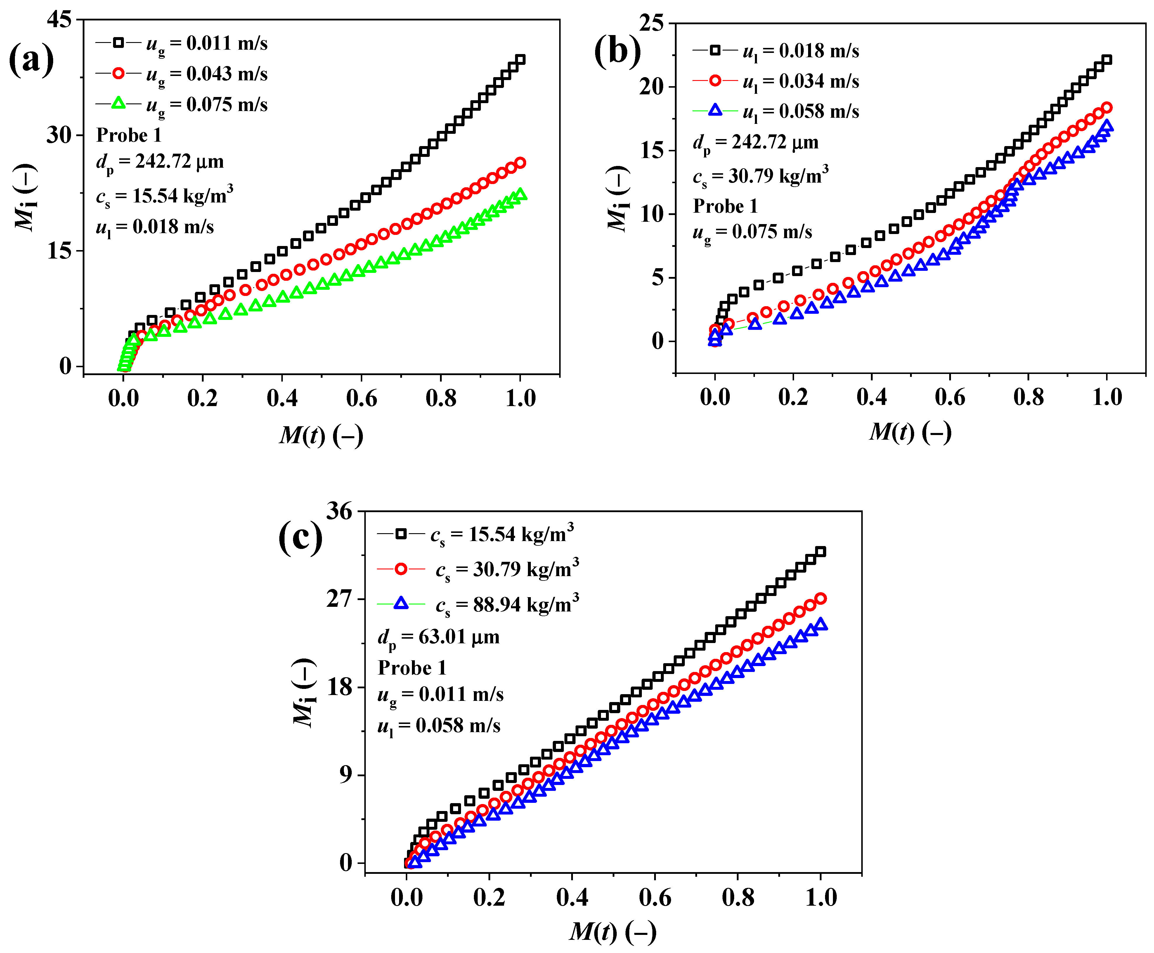
4.2. Dependency of the Intrinsic MT Number on the QM

Intrinsic MT number $\left(M_{\mathrm{i}}\right)$ as a function of the QM in the various experimental conditions is shown in Figure 4a–c. As expected, the increase in $M_{\mathrm{i}}$ was accompanied by an increase in $M\left(t\right)$ for all experimental conditions. It is observed that $M_{\mathrm{i}}$ reduces as the gas velocity increases, as shown in Figure 4a. As the gas velocity increases, the coalescence rate of the bubble also increases, hence the bubble size. The interfacial area of contact between the gas and slurry decreases as the bubble size increases. As a result, $M_{\mathrm{i}}$ decreases. The influence of slurry velocity on $M_{\mathrm{i}}$ is demonstrated in Figure 4b. It can be seen that the $M_{\mathrm{i}}$ reduces as the velocity of the slurry increases. The $M_{\mathrm{i}}$ reflects the MT between the bubble and the slurry. The contact time between the bubble and slurry decreases as the slurry velocity increases while the circulation and turbulence accelerate. The reduced contact time and increased circulation and turbulence reduce the $M_{\mathrm{i}}$. The influence of particle loading on the $M_{\mathrm{i}}$ is displayed in Figure 4c. The $M_{\mathrm{i}}$ is higher at a lower particle loading $(c_{\mathrm{s}}=15.54\mathrm{kg}/{\mathrm{m}}^3)$, and it decreases as the particle loading increases from $c_{\mathrm{s}}=15.54\mathrm{to}88.94\mathrm{kg}/{\mathrm{m}}^3$. It is obvious that the increase in particle loading increases the viscosity of the system, thereby decreasing the intensity of the turbulence. Reduced turbulence leads to the formation of a laminar film boundary layer between the bubble and the slurry. Therefore, the $M_{\mathrm{i}}$ decreases.

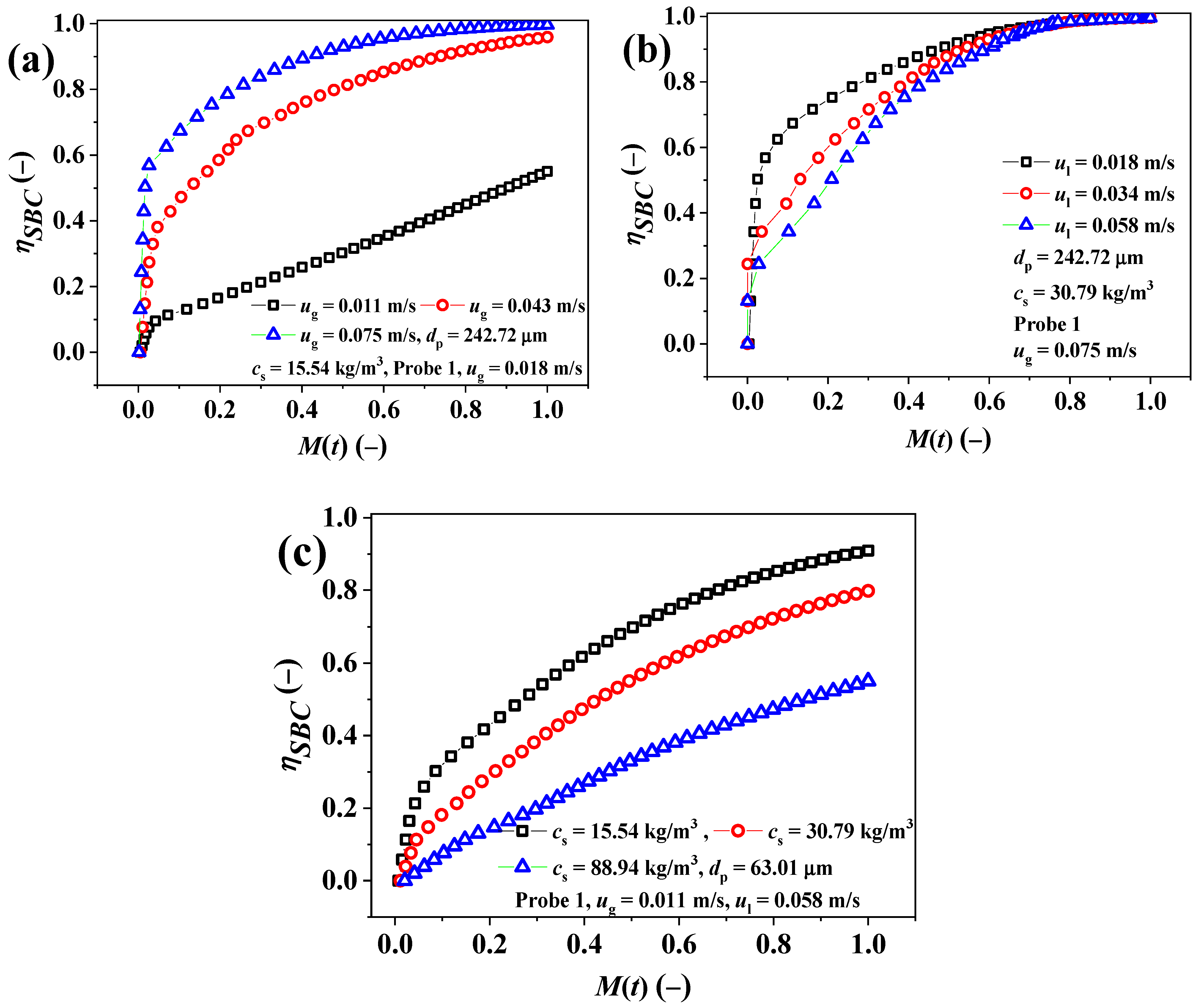
4.3. Mass Transfer (MT) Efficiency Based on the QUALITY of Mixedness (QM)

For MT studies in the gas–slurry system, the slurry-side MT coefficient and the QM are considered the most important transport properties. MT efficiency based on the IE theory in the three-phase co-current downflow BC has also been reported by other researchers [34]. At a complete mixing condition, the MT rate is given as

$$\frac{d{c}_{\mathrm{l}}}{dt}=k_{\mathrm{s}\mathrm{l}}a\left(c_{\mathrm{l}}^{\mathrm{e}}-c_{\mathrm{l}}\right)$$

(29)

In integral form, Equation (29) can be written as

$${\int }_{c_{\mathrm{l},h_{\mathrm{i}-1}}}^{c_{\mathrm{l},h_{\mathrm{i}}}}\frac{d{c}_{\mathrm{l}}}{c_{\mathrm{l}}^{\mathrm{e}}-c_{\mathrm{l}}}=k_{\mathrm{s}\mathrm{l}}a{\int }_{t_{\mathrm{i}-1}}^{t_{\mathrm{i}}}dt$$

(30)

After integration with suitable boundary conditions, Equation (30) can be written as

$$\frac{c_{\mathrm{l},h_{\mathrm{i}}}-c_{\mathrm{l},h_{\mathrm{i}-1}}}{c_{\mathrm{l},h_{\mathrm{i}}}^{\mathrm{e}}-c_{\mathrm{l},h_{\mathrm{i}-1}}}=1-e^{-k_{\mathrm{s}\mathrm{l}}a{t}_{\mathrm{i},\mathrm{i}-1}}$$

(31)

The equilibrium concentration $\left(c_{\mathrm{l},h_{\mathrm{i}}}^e\right)$ in the slurry as a function of the gas–slurry dispersion height can be defined as

$$c_{\mathrm{l},h_{\mathrm{i}}}^{\mathrm{e}}\lambda =P_{{\mathrm{h}}_{\mathrm{i}}}{y}_{{\mathrm{h}}_{\mathrm{i}}}$$

(32)

where $\lambda$ and $P_{{\mathrm{h}}_{\mathrm{i}}}$ denotes Henry’s law constant and the pressure at various axial heights in the column. The pressure $\left(P_{{\mathrm{h}}_{\mathrm{i}}}\right)$ as a function of the total pressure $\left(P_{\mathrm{t}}\right)$, the ratio between the hydrostatic pressure and the total pressure of the column $\left(\beta \right)$, and the dimensionless height $(h_{\mathrm{r},\mathrm{i}}=h_{\mathrm{i}}/h_{\mathrm{m}})$ can be represented as

$$P_{\mathrm{h},\mathrm{i}}=\left(1+\beta (1-h_{\mathrm{r},\mathrm{i}})\right)P_{\mathrm{t}}$$

(33)

The total column pressure can be defined as

$$P_{\mathrm{t}}=\left(P_{\mathrm{a}\mathrm{t}\mathrm{m}}\right)+\left({\rho }_{\mathrm{s}\mathrm{l}}g{h}_{\mathrm{i}}\right)+\left(4{\sigma }_{\mathrm{s}\mathrm{l}}/d_{32}\right)$$

(34)

The ratio $\left(\beta \right)$ between the hydrostatic pressure and the total pressure of the column can be calculated as follows:

$$\beta =\frac{1-{\alpha }_{\mathrm{g}}}{P_{\mathrm{r}}+h_{\mathrm{r},\mathrm{i}}+{\gamma }_{\mathrm{b}}}$$

(35)

where $P_{\mathrm{r}}=P_{\mathrm{t}}/{\rho }_{\mathrm{s}\mathrm{l}}g{h}_{\mathrm{m}}$ and ${\gamma }_{\mathrm{b}}=4{\sigma }_{\mathrm{s}\mathrm{l}}/{\rho }_{\mathrm{s}\mathrm{l}}g{h}_{\mathrm{m}}{d}_{32}$. The substitution of Equation (33) into Equation (32) yields the equilibrium concentration at a fixed gas-phase molar concentration

$$c_{\mathrm{l},h_{\mathrm{i}}}^{\mathrm{e}}=\frac{1}{\lambda }{P}_{\mathrm{t}}\left[1+\beta (1-h_{\mathrm{r},\mathrm{i}})\right]y_{\mathrm{h},\mathrm{i}}$$

(36)

Solution and saturation concentrations vary axially in the column. The local MT efficiency $\left({\eta }_{{\mathrm{h}}_{\mathrm{i}-1}}^{{\mathrm{h}}_{\mathrm{i}}}\right)$ at a fixed height can be given as

$${\eta }_{{\mathrm{h}}_{\mathrm{i}-1}}^{h_{\mathrm{i}}}=\frac{c_{\mathrm{l},{\mathrm{h}}_{\mathrm{i}}}-c_{\mathrm{l},{\mathrm{h}}_{\mathrm{i}-1}}}{c_{\mathrm{l},{\mathrm{h}}_{\mathrm{i}}}^e-c_{\mathrm{l},{\mathrm{h}}_{\mathrm{i}-1}}}$$

(37)

From Equations (31) and (37), ${\eta }_{{\mathrm{h}}_{\mathrm{i}-1}}^{{\mathrm{h}}_{\mathrm{i}}}$ can be defined as

$${\eta }_{{\mathrm{h}}_{\mathrm{i}-1}}^{{\mathrm{h}}_{\mathrm{i}}}=\frac{c_{\mathrm{l},{\mathrm{h}}_{\mathrm{i}}}-c_{\mathrm{l},{\mathrm{h}}_{\mathrm{i}-1}}}{c_{\mathrm{l},{\mathrm{h}}_{\mathrm{i}}}^{\mathrm{e}}-c_{\mathrm{l},{\mathrm{h}}_{\mathrm{i}-1}}}=1-e^{-k_{\mathrm{s}\mathrm{l}}a{t}_{\mathrm{i},\mathrm{i}-1}}$$

(38)

If the average bulk concentration of liquid at the inlet and outlet is $c_{\mathrm{l},{\mathrm{h}}_{\mathrm{i}\mathrm{n}}}$ and $c_{\mathrm{l},{\mathrm{h}}_{\mathrm{o}\mathrm{u}\mathrm{t}}}$, respectively, then the MT efficiency of the whole column can be represented as

$${\eta }_{\mathrm{S}\mathrm{B}\mathrm{C}}=\frac{c_{\mathrm{l},{\mathrm{h}}_{\mathrm{m}}}-c_{\mathrm{l},{\mathrm{h}}_{\mathrm{i}\mathrm{n}}}}{c_{\mathrm{l},{\mathrm{h}}_{\mathrm{m}}}^{\mathrm{e}}-c_{\mathrm{l},{\mathrm{h}}_{\mathrm{i}\mathrm{n}}}}=1-e^{-k_{\mathrm{s}\mathrm{l}}a{t}_{\mathrm{i},\mathrm{i}-1}}$$

(39)

MT efficiency of the SBC depends on the QM. Therefore, the overall efficiency of the column as a function of the QM can be represented as

$${\eta }_{\mathrm{S}\mathrm{B}\mathrm{C}}=\frac{c_{\mathrm{l},{\mathrm{h}}_{\mathrm{m}}}-c_{\mathrm{l},{\mathrm{h}}_{\mathrm{i}\mathrm{n}}}}{c_{\mathrm{l},{\mathrm{h}}_{\mathrm{m}}}^{\mathrm{e}}-c_{\mathrm{l},{\mathrm{h}}_{\mathrm{i}\mathrm{n}}}}=1-\mathit{exp}\left[\frac{E_{\mathrm{z}}{\alpha }_{\mathrm{g}}}{k_{\mathrm{s}\mathrm{l}}{d}_{32}\left(A\right(1-M\left(t\right)){)}^{\mathrm{B}}}\right]$$

(40)

where A and B are the constants, which can be estimated from the experimental values. The effect of the QM on the MT efficiency $\left({\eta }_{\mathrm{S}\mathrm{B}\mathrm{C}}\right)$ of the counter-current SBC is illustrated in Figure 5a–c. It is observed that the ${\eta }_{\mathrm{S}\mathrm{B}\mathrm{C}}$ increases with the QM $\left(M\right(t\left)\right)$ for all experimental conditions. It is noticed that the $M\left(t\right)$ increases as the gas velocity increases, as shown in Figure 5a. The increase in ${\eta }_{\mathrm{S}\mathrm{B}\mathrm{C}}$ is attributed to the higher interaction between bubbles and slurry in the column. Figure 5b shows that the ${\eta }_{\mathrm{S}\mathrm{B}\mathrm{C}}$ is higher for u_l = 0.018 m/s compared to other slurry velocities $(u_{\mathrm{l}}=0.034\mathrm{and}0.058\mathrm{m}/\mathrm{s})$, up to M(t) = 0.8. After $M\left(t\right)=0.8$, the ${\eta }_{\mathrm{S}\mathrm{B}\mathrm{C}}$ is almost equal to all other slurry velocities. Although it has been observed that the $M\left(t\right)$ as a function of dimensionless time $(t/t_{\mathrm{c}})$ is greater at a higher slurry velocity (as shown in Figure 5b), the ${\eta }_{\mathrm{S}\mathrm{B}\mathrm{C}}$ as a function of increased slurry velocity decreases. The reason may be that the higher slurry velocity may not facilitate sufficient contact time for MT between the bubble and the slurry. The effect of particle loading on ${\eta }_{\mathrm{S}\mathrm{B}\mathrm{C}}$ is shown in Figure 5c. As observed, there is a significant difference in the ${\eta }_{\mathrm{S}\mathrm{B}\mathrm{C}}$ curve at different solid loadings. The increase in the loading of the particles significantly changes the viscosity of the slurry. Therefore, the intensity of the coalescence of the bubbles increases. The increase in bubble size results in a low interfacial area between the bubble and the slurry and a low MT rate. The increased slurry viscosity reduces the degree of turbulence in the column, which, in turn, reduces the collision of particles with the effective boundary layer thickness between the gas and the slurry [34]. Hence, the ${\eta }_{\mathrm{S}\mathrm{B}\mathrm{C}}$ reduces.

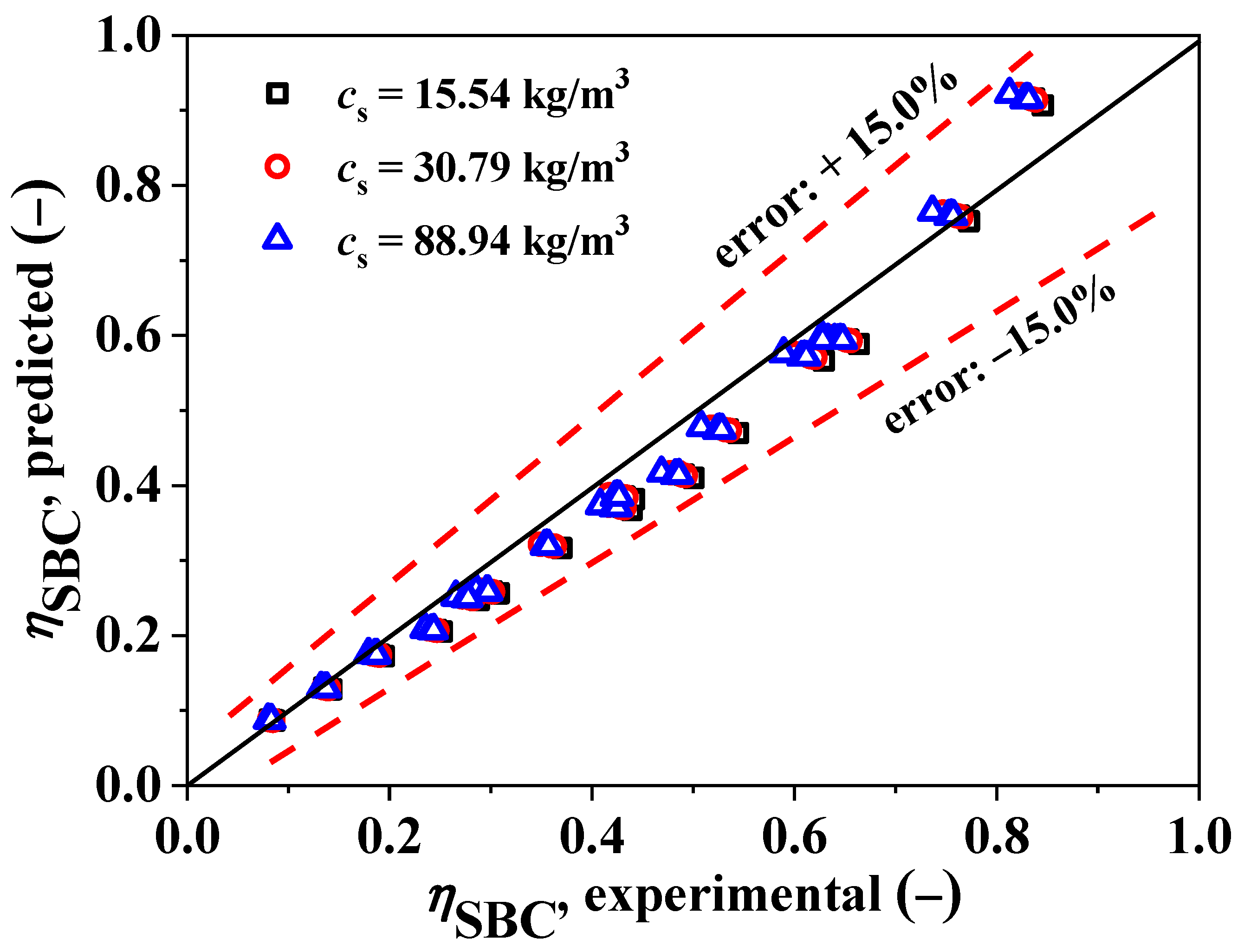
Prediction of MT Efficiency

For predicting MT efficiency, an empirical correlation is developed by taking into account the inlet gas velocity $\left(u_{\mathrm{g}}\right)$, the inlet slurry velocity $\left(u_{\mathrm{l}}\right)$, the column diameter $\left(d_{\mathrm{c}}\right)$, the slurry density $\left({\rho }_{\mathrm{s}\mathrm{l}}\right)$, the slurry surface tension $\left({\mathsf{\sigma }}_{\mathrm{s}\mathrm{l}}\right)$, and the acceleration due to gravity $\left(g\right)$. MT efficiency as a function of different dimensionless groups is given as

$${\eta }_{SBC}=\varphi {\left(\frac{{\rho }_{sl{u}_l^2{d}_c}}{{\sigma }_{sl}}\right)}^b{\left(\frac{g_{d_c}}{u_g^2}\right)}^c$$

(41)

The values of $\varphi$, $b$, and $c$ are obtained after regression analysis as 3.11, −0.37, and −0.39, respectively. The final form of Equation (41) is given as

$${\eta }_{SBC}=3.11{\left(\frac{{\rho }_{sl{u}_l^2{d}_c}}{{\sigma }_{sl}}\right)}^{-0.37}{\left(\frac{g_{d_c}}{u_g^2}\right)}^{-0.39}$$

(42)

The range of parameters is $0.229\le {\rho }_{sl}{u}_l^2{d}_c/{\sigma }_{sl}\le 2.489$; $91.445\le g{d}_c/u_g^2\le 4122.477$. The predicted values are in the range of ±15.0% error and 9.22% absolute average relative error (AARE). The correlation coefficient (R²) of Equation (42) was 0.99. The parity plot of ${\eta }_{\mathrm{S}\mathrm{B}\mathrm{C}}$ is shown in Figure 6.

5. Conclusions

The present research reports the QM, the MT number, and the overall MT efficiency based on the IE theory in the three-phase counter-current microstructured bubble column. The importance and significance of IE theory and the algorithm for IE calculation have been clearly explained. The IE definition is based on the probability distribution when observing a specific event. The slurry-phase mixing characteristics are reported in relation to the QM. An in-depth analysis was conducted to understand the influence of gas velocity, slurry velocity, solid loading, and axial height on the QM, MT number, and overall MT efficiency. It was noted that these variables have an intense effect on the QM. Based on the analysis, the following conclusions can be drawn:

• The QM parameter based on the IE in various experimental conditions varies between 0 (the minimum value) and 1 (the ultimate value). The QM is a time-dependent parameter. For scale-up purposes, time is made dimensionless $(t/t_c)$, such as the ratio of time and contact time between bubbles and slurry. The QM is modeled as a function of the Sherwood and the intrinsic MT numbers. The inlet gas and slurry velocity positively affect the QM, while particle loading and the axial height reduce the QM. The QM is higher in the sparger region compared to the other axial positions. The QM in the transverse direction is maximum at the central part of the column compared to other transverse positions.
• The intrinsic MT number exhibits an efficient MT from the gas phase to the liquid phase over a specified contact period. It depends on the interfacial contact area between the gas and slurry phases and the average contact time. The intrinsic MT number decreases as the inlet slurry velocity rate and particle loading increase, whereas it intensifies with an increase in the inlet gas velocity.
• The overall MT efficiency was presented as a function of the QM based on the IE theory. Increasing the inlet gas velocity enhances the overall MT efficiency. However, it reduces as the inlet slurry velocity and particle loading increase.
• The mixing results can help better understand intensify the processes, and model the counter-current microstructured SBCs in industrial applications.

References

1. Deckwer, W.-D. Bubble Column Reactors; Wiley: Chichester, UK, 1992. [Google Scholar]
2. Emami, A.; Briens, C. A method for the detection of defluidized zones in slurry bubble columns. Can. J. Chem. Eng. 2003, 81, 451–455. [Google Scholar] [CrossRef]
3. Muhsin, H.A.A.-k.; Mohammad, F.A. Experimental study of liquid dispersion in bubble column. Diyala J. Eng. Sci. 2008, 1, 56–85. [Google Scholar] [CrossRef]
4. Wadaugsorn, K.; Limtrakul, S.; Vatanatham, T.; Ramachandran, P.A. Mixing characteristics of gas and liquid phases in bubble column reactors from virtual tracer simulation. Ind. Eng. Chem. Res. 2018, 57, 14064–14079. [Google Scholar] [CrossRef]
5. Ekambara, K.; Joshi, J.B. CFD simulation of mixing and dispersion in bubble columns. Chem. Eng. Res. Des. 2003, 81, 987–1002. [Google Scholar] [CrossRef]
6. Bhusare, V.H.; Kalaga, D.V.; Dhiman, M.K.; Joshi, J.B.; Roy, S. Mixing in a co-current upflow bubble column reactors with and without internals. Can. J. Chem. Eng. 2018, 96, 1957–1971. [Google Scholar] [CrossRef]
7. Ansari, M.; Turney, D.E.; Yakobov, R.; Kalaga, D.V.; Kleinbart, S.; Banerjee, S.; Joshi, J.B. Chemical hydrodynamics of a downward microbubble flow for intensification of gas-fed bioreactors. AIChE J. 2018, 64, 1399–1411. [Google Scholar] [CrossRef]
8. Pareek, V.K.; Yap, Z.; Brungs, M.P.; Adesina, A.A. Particle residence time distribution (RTD) in three-phase annular bubble column reactor. Chem. Eng. Sci. 2001, 56, 6063–6071. [Google Scholar] [CrossRef]
9. Kumar, R.; Pant, H.J.; Goswami, S.; Sharma, V.K.; Dash, A.; Mishra, S.; Bhanja, K.; Mohan, S.; Mahajani, S.M. Investigation of holdup and axial dispersion of liquid phase in a catalytic exchange column using radiotracer technique. Appl. Radiat. Isot. 2017, 121, 51–60. [Google Scholar] [CrossRef]
10. Shah, M.; Kiss, A.A.; Zondervan, E.; Van der Schaaf, J.; De Haan, A.B. Gas holdup, axial dispersion, and mass transfer studies in bubble columns. Ind. Eng. Chem. Res. 2012, 51, 14268–14278. [Google Scholar] [CrossRef]
11. Ekambara, K.; Dhotre, M.T. CFD simulation of bubble column. Nucl. Eng. Des. 2010, 240, 963–969. [Google Scholar] [CrossRef]
12. Shaikh, A.; Al-Dahhan, M. Scale-up of bubble column reactors: A review of current state-of-the-art. Ind. Eng. Chem. Res. 2013, 52, 8091–8108. [Google Scholar] [CrossRef]
13. Gao, Y.; Muzzio, F.J.; Ierapetritou, M.G. A review of the Residence Time Distribution (RTD) applications in solid unit operations. Powder Technol. 2012, 228, 416–423. [Google Scholar] [CrossRef]
14. Palaskar, S.N.; De, J.K.; Pandit, A.B. Liquid phase RTD studies in sectionalized bubble column. Chem. Eng. Technol. 2000, 23, 61–69. [Google Scholar] [CrossRef]
15. Bhatia, B.; Nigam, K.D.P.; Auban, D.; Hebrard, G. Effect of a new high porosity packing on hydrodynamics and mass transfer in bubble columns. Chem. Eng. Process. Process Intensif. 2004, 43, 1371–1380. [Google Scholar] [CrossRef]
16. Wu, Y.; Cheng, Z.-M.; Huang, Z.-B. Backmixing reduction of a bubble column by interruption of the global liquid circulation. Ind. Eng. Chem. Res. 2009, 48, 6558–6563. [Google Scholar] [CrossRef]
17. Forret, A.; Schweitzer, J.M.; Gauthier, T.; Krishna, R.; Schweich, D. Liquid dispersion in large diameter bubble columns, with and without internals. Can. J. Chem. Eng. 2003, 81, 360–366. [Google Scholar] [CrossRef]
18. Agahzamin, S.; Pakzad, L. CFD investigation of the gas dispersion and liquid mixing in bubble columns with dense vertical internals. Chem. Eng. Sci. 2019, 203, 425–438. [Google Scholar] [CrossRef]
19. Belfares, L.; Cassanello, M.; Grandjean, B.P.; Larachi, F.ç. Liquid back-mixing in packed-bubble column reactors: A state-of-the-art correlation. Catal. Today 2001, 64, 321–332. [Google Scholar] [CrossRef]
20. Eissa, S.H.; Schügerl, K. Holdup and backmixing investigations in cocurrent and countercurrent bubble columns. Chem. Eng. Sci. 1975, 30, 1251–1256. [Google Scholar] [CrossRef]
21. Abdulrazzaq, B.S. Gas holdup and axial liquid dispersion in three phase bubble columns. J. Eng. Sustain. Dev. 2015, 19, 132–146. [Google Scholar]
22. Forret, A.; Schweitzer, J.M.; Gauthier, T.; Krishna, R.; Schweich, D. Scale up of slurry bubble reactors. Oil Gas Sci. Technol. 2006, 61, 443–458. [Google Scholar] [CrossRef]
23. Kelkar, B.G.; Shah, Y.T.; Carr, N.L. Hydrodynamics and axial mixing in a three-phase bubble column. Effects of slurry properties. Ind. Eng. Chem. Process Des. Dev. 1984, 23, 308–313. [Google Scholar] [CrossRef]
24. Prakash, R.; Majumder, S.K.; Singh, A. Dispersion characteristics in a counter-current microstructured slurry bubble column and its analysis based on the turbulence and circulation. Ind. Eng. Chem. Res. 2020, 59, 8093–8111. [Google Scholar] [CrossRef]
25. Ityokumbul, M.T.; Kosaric, N.; Bulani, W. Effect of fine solids and frother on gas hold-up and liquid mixing in a flotation column. Miner. Eng. 1995, 8, 1369–1380. [Google Scholar] [CrossRef]
26. Rubio, F.C.; Mirón, A.S.; García, M.-C.C.; Camacho, F.G.; Grima, E.M.; Chisti, Y. Mixing in bubble columns: A new approach for characterizing dispersion coefficients. Chem. Eng. Sci. 2004, 59, 4369–4376. [Google Scholar] [CrossRef]
27. Nedeltchev, S.; Ookawara, S.; Ogawa, K. A fundamental approach to bubble column scale-up based on quality of mixedness. J. Chem. Eng. Jpn. 1999, 32, 431–439. [Google Scholar] [CrossRef]
28. Li, W.-L.; Zhong, W.-Q.; Jin, B.-S.; Xiao, R.; He, T.-T. Flow regime identification in a three-phase bubble column based on statistical, Hurst, Hilbert–Huang transform and Shannon entropy analysis. Chem. Eng. Sci. 2013, 102, 474–485. [Google Scholar] [CrossRef]
29. Zhang, X.; Guo, K.; Qi, W.; Zhang, T.; Liu, C. Gas holdup, bubble behaviour, and mass transfer characteristics in a two-stage internal loop airlift reactor with different screens. Can. J. Chem. Eng. 2017, 95, 1202–1212. [Google Scholar] [CrossRef]
30. Prakash, R.; Bhattacharyya, A.; Majumder, S.K. Experimental investigation and its analysis of gas holdup in a three-phase counter-current microstructured bubble column. J. Dispers. Sci. Technol. 2022, 43, 243–258. [Google Scholar] [CrossRef]
31. Fan, L.S.; Tsuchiya, K. Bubble Wake Dynamics in Liquid and Liquid-Solid Suspensions, Butter-Worth-Heinemann Series in Chemical Engineering; Elsevier: Amsterdam, The Netherlands, 1990. [Google Scholar]
32. Clift, R.; Grace, J.R.; Weber, M.E. Bubbles, Drops and Particles; Academic Press: New York, NY, USA, 1978. [Google Scholar]
33. Nedeltchev, S.; Jordan, U.; Schumpe, A. A new correction factor for theoretical prediction of mass transfer coefficients in bubble columns. J. Chem. Eng. Jpn. 2006, 39, 1237–1242. [Google Scholar] [CrossRef]
34. Majumder, S.K. Hydrodynamics and Mass Transfer in Downflow Slurry Bubble Columns; CRC Press: Waretown, NJ, USA, 2019. [Google Scholar]
Figure 1. Schematic configuration of the experimental setup (adapted with permission from Prakash et al. [24]). The conductivity probes were 1, 2, 3, and 4 in the axial direction, and probes 2, 5, and 6 in the transverse direction.
Processes 12 00281 g001
Figure 2. Quality of mixedness as a function of time.
Processes 12 00281 g002
Figure 3. Variation in QM with dimensionless time: influence of (a) u g , (b) u l , (c) c s , and (d) aspect ratios.
Processes 12 00281 g003aProcesses 12 00281 g003b
Figure 4. Variation in Mi as a function of (a) the gas velocity, (b) the slurry velocity, and (c) the particle loading.
Processes 12 00281 g004
Figure 5. Variation in η S B C as a function of (a) gas velocity, (b) slurry velocity, and (c) particle loading.
Processes 12 00281 g005
Figure 6. Parity plot of the overall MT efficiency.
Processes 12 00281 g006
Disclaimer/Publisher’s Note: The statements, opinions and data contained in all publications are solely those of the individual author(s) and contributor(s) and not of MDPI and/or the editor(s). MDPI and/or the editor(s) disclaim responsibility for any injury to people or property resulting from any ideas, methods, instructions or products referred to in the content.