Feature Extraction and Diagnosis of Periodic Transient Impact Faults Based on a Fast Average Kurtogram–GhostNet Method

Abstract

This paper proposes an improved fault diagnosis algorithm that combines a modified fast kurtogram (FK) method with the lightweight convolutional neural network GhostNet. The FK algorithm can adaptively select resonance demodulation bands for envelope demodulation to extract fault features, but it may be disturbed by non-Gaussian noise. Hence, the fast average kurtogram (FAK) method based on sub-band averaging was introduced. This method effectively weakens the impact of pulse noise on the kurtosis graph by splitting the signal into equal-length sub-signals and calculating the average kurtosis value of all sub-signal filters. Simultaneously, to fully utilize the advantages of deep learning technology in feature extraction and classification, this study used the FAK to convert vibration signals from one-dimensional to two-dimensional kurtosis graphs as the input for the GhostNet model. This combination not only achieved accurate fault diagnosis and classification but also showed significant advantages in processing efficiency and resource utilization. The experimental results indicate that the algorithm excelled in extracting features and diagnosing periodic transient impact faults, and compared with traditional methods, it exhibited noticeable improvements in computational efficiency and resource management.

1. Introduction

In the context of today’s industrial automation and intelligent manufacturing, there are higher requirements for mechanical equipment health monitoring and fault diagnosis technology. Given the increasing maturity of technologies, such as the industrial Internet of things, mobile Internet and cloud computing, the combination of these technologies brings new opportunities to the mechanical fault diagnosis field. In practical applications, rotating machinery fault diagnosis, especially for critical components, such as gears, bearings and rotors, remains a challenge. Therefore, the development of intelligent fault diagnosis technology that can accurately and efficiently diagnose these critical components is crucial to improving equipment reliability and safety [1].

Spectral kurtosis (SK), which is an efficient signal processing method, was first proposed by Dwyer for frequency domain analysis [2]. Antoni further refined the mathematical definition of spectral kurtosis and introduced the fast kurtogram (FK), which has been successfully applied to vibration monitoring and fault detection in rolling bearings. Additionally, Lei and others [3] suggested replacing the finite impulse response filters in FK with wavelet packet transform, utilizing its local characteristics in time and frequency spaces for more accurate fault feature extraction. However, the wavelet packet transform can be affected by boundary effects, leading to inaccurate analysis results. Zhang Y and Randall R B [4] combined FK with genetic algorithms to optimize the resonance demodulation parameters in bearing fault diagnosis. This resolved the issue of not being able to independently select the filter center frequency and bandwidth, thus enhancing the diagnostic precision. However, genetic algorithms often involve extensive iterations and computations, potentially increasing the computational costs when dealing with large amounts of data. Studies showed that FK is easily disturbed by non-Gaussian noise, which can mask or confuse the signal features caused by faults, thus affecting the accuracy of fault diagnosis [5,6]. To address this, Dai and others [7] proposed a fast spectral kurtosis algorithm based on sub-band spectral kurtosis averaging, effectively mitigating pulse interference. Building on this, Wang L and others [8] replaced the wavelet packet with dual-tree complex wavelet packets in FK. The use of two orthogonally oriented wavelet trees can effectively capture local features of the signal, reducing impacts due to signal shifts. This method greatly reduces the impact of non-Gaussian noise and achieves good results in diagnosing faults in planetary gearboxes and rolling bearings.

However, traditional signal processing typically requires manual feature engineering and has limited generalization capabilities. Deep learning can compensate for these shortcomings, providing stronger data analysis and pattern recognition capabilities, especially when dealing with large-scale and variable data. Deep learning models, particularly convolutional neural networks (CNNs), have become a hot topic in the field of intelligent fault diagnosis [9]. Wang and others [10] combined CNNs with long short-term memory networks to propose an improved method for bearing fault diagnosis. Huang and others [11] introduced a multi-scale convolutional network that enhanced the model’s expressive power by adding a multi-scale cascading layer in front of the regular CNN, but this also significantly increased the computational load, making it difficult to deploy the model on resource-limited mobile or embedded devices. To address efficiency and storage issues, lightweight network designs, like MobileNet, ShuffleNet and SqueezeNext, emerged [12,13,14]. Although these models achieve remarkable performance with minimal floating points, they do not fully utilize the correlations and redundancies between feature maps. Han and others [15] introduced a lightweight Ghost convolutional neural network (GhostNet), which replaced standard convolution operations with low-rank linear transformations and group convolution-based residual connections. This significantly reduced the computational costs and parameter count while maintaining accuracy. Combining lightweight networks with signal processing technology can provide a more powerful and intelligent solution for fault diagnosis and prevention.

In summary, this paper proposes a new fault diagnosis method based on FAK-GhostNet, aiming to overcome the limitations of existing technologies. By averaging the kurtosis of sub-signal band-pass filters, this method effectively eliminates the impact of non-Gaussian noise. Using the two-dimensional features extracted from different faults by the FAK algorithm, it successfully applies them to the GhostNet model for fault identification and classification. Experimental validation on critical components of rotating machinery not only confirmed the effectiveness of the proposed method but also demonstrated its significant advantages in improving the accuracy and efficiency of fault diagnosis.

2. Optimized Algorithm Based on the Fast Kurtogram

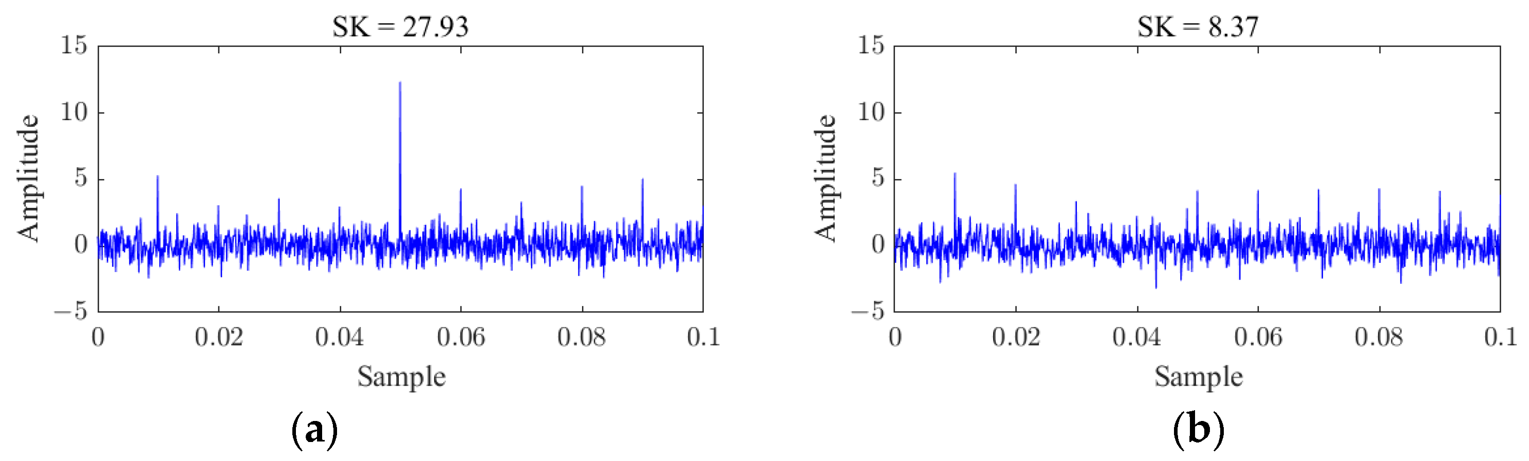
2.1. Spectral Kurtosis Definition

Spectral kurtosis characterizes a signal’s non-Gaussianity through its frequency domain statistical properties. It is commonly used in nonlinear systems analysis, fault diagnosis, biomedical signal analysis and other fields. In the time domain, kurtosis is typically expressed as

$$K\left(x\right)=\frac{〈{\left(x-\mu \right)}^4〉}{{\sigma }^4}-3$$

(1)

In the formula, $\mu$ is the mean, $\sigma$ is the standard deviation and $〈·〉$ denotes the expected value.

Kurtosis is a statistic that describes a signal’s distribution shape in the time domain; spectral kurtosis converts a signal from the time domain to the frequency domain for analysis, reflecting the change in signal kurtosis value with frequency. According to Antoni, the $Wold-Gram\acute{e}r$ decomposition of the zero-mean nonstationary signal $x\left(t\right)$ is defined as

$$x(t)={\displaystyle \underset{-1/2}{\overset{1/2}{\int }}{e}^{j2\pi fn}H(t,f)d{Z}_x(f)}$$

(2)

In this formula, $H(t,f)$ is the complex envelope of signal $x\left(t\right)$ at frequency $f$, $d{Z}_x\left(f\right)$ is the orthogonal spectral increment and $e^{j2\pi fn}H(t,f)d{Z}_x\left(f\right)$ is the output of an infinitely narrow band filter centered at frequency $f$. The definition of spectral kurtosis can then be expressed as [16]

$$K_x(f)=\frac{〈{\left|H(t,f)\right|}^4〉}{{〈{\left|H(t,f)\right|}^2〉}^2}-2$$

(3)

In this formula, $〈{\left|H\left(t,f\right)\right|}^2〉$ represents the second-order moment, indicating the signal’s energy, and $〈{\left|H\left(t,f\right)\right|}^4〉$ stands for the fourth-order moment, which depicts the kurtosis of the power spectrum. This equation describes the shape of the signal’s power spectrum at frequency $f$.

2.2. Fast Kurtogram Algorithm Definition

The fast spectral kurtosis algorithm, which was developed to address the high computational cost of traditional spectral kurtosis methods when dealing with large datasets, operates by decomposing signals using a predefined filter bank. This approach seeks the optimal combination of frequency and frequency resolution across the entire frequency band plane, enabling the precise determination of the frequency band position and the interval for transient impact components. This algorithm’s primary implementation steps include the following [17]:

• As shown in Equations (4) and (5), two quasi-analytic filters are constructed, namely, a low-pass filter $h_0\left(n\right)$ and high-pass filter $h_1\left(n\right)$, where $h\left(n\right)$ is a low-pass filter with a cutoff frequency $f_c=\frac{1}{8}+\epsilon (\epsilon \ge 0)$; $h_0\left(n\right)$ is a quasi-analytic low-pass filter with a bandwidth of $\left[\mathrm{0,1}/4\right]$ and the frequency shift of $h\left(n\right)$ is 0.125; $h_1\left(n\right)$ is a quasi-analytic high-pass filter with a bandwidth of $\left[1/4, 1/2\right]$ obtained via a frequency shift of 0.375 from $h\left(n\right)$.

  $$h_0(n)=h(n)e^{j\pi n/4}$$

  (4)

  $$h_1(n)=h(n)e^{3j\pi n/4}$$

  (5)
• As shown in Figure 1a, the filters $h_0\left(n\right)$ and $h_1\left(n\right)$ are used to filter the signal, and the twofold downsampling method is adopted for iteration to keep the total amount of data unchanged. In Figure 1a, $c_l^i(n)$ is the coefficient sequence of the $i$th filter at the $l$th level $(i=0,\dots ,2^l-1, l=0,\dots ,L-1)$, where $L$ is the number of decomposition levels of the filter, and two new sequences $c_{l+1}^{2i}(n)$ and $c_{l+1}^{2i+1}(n)$ are generated in layer $l+1$ after filtering. It is worth noting that multiplying the $h_1\left(n\right)$ filter by ${(-j)}^n$ is to convert the high-pass sequence to the low-pass sequence, thus complying with the frequency ordering. This process iterates from layer $l=0$ and continues to $L-1$, resulting in a tree-like filter bank at each layer with $2^l$ sub-bands, as shown in Figure 1b. Therefore, the coefficient $c_l^i(n)$ can be interpreted as a complex envelope of the signal $x\left(n\right)$ located at the central frequency $f_i$, and $∆f$ is the bandwidth.

  $$f_i=(i+2^{-1})2^{-l-1}$$

  (6)

  $$(\Delta f)=2^{-k-1}$$

  (7)
• The spectral kurtosis value of each frequency band is calculated. From Formula (3), the spectral kurtosis of the complex envelope ci can be calculated at the center frequency $f_i$ with bandwidth $∆f$. Therefore, Formula (3) can be rewritten as

  $$K_l^i=\frac{〈{\left|c_l^i(n)\right|}^4〉}{{〈{\left|c_l^i(n)\right|}^2〉}^2}-2$$

  (8)

2.3. Fast Averaging Kurtogram Algorithm Definition

The FK algorithm, as an efficient tool for detecting and analyzing non-steady-state components of vibration signals, is often used in rotating machinery fault diagnosis. The algorithm can adaptively determine the optimal demodulation frequency band of the shock signal related to a fault and realize the fault signal’s location and analysis. However, as shown in Figure 2, the FK method is susceptible to pulse interference with a large kurtosis value in the vibration signal, which interferes with the accuracy of the optimal frequency band selection. Studies showed that frequency–domain averaging is commonly used to improve the SNR and can effectively remove non-periodic random interference in the spectrum [18]. To address this, this section proposes a new method that applies an equalization approach to spectral kurtosis to eliminate the impact of pulse interferences, termed the fast average kurtogram (FAK) algorithm. The main steps of this algorithm are as follows:

• Original signal segmentation by dividing the vibration signal x(t) into M equal-length sub-signals {x_m (t)|m = 1,2, …, M}.
• Sub-signal spectral kurtosis value calculation of the kurtosis values of each sub-signal after the dual-tree complex wavelet packet transform (DTCWPT):

  $$K_x(f)=\frac{〈{\left|H(t,f)\right|}^4〉}{{〈{\left|H(t,f)\right|}^2〉}^2}-2$$

  (9)
• Average the kurtosis values of each sub-band and sum the corresponding positions of the M group spectral kurtosis arrays obtained in the previous step to find the average:

  $$\overline{K}=\frac{1}{M}{\displaystyle {\sum }_{m=1}^M}{K}_m$$

  (10)
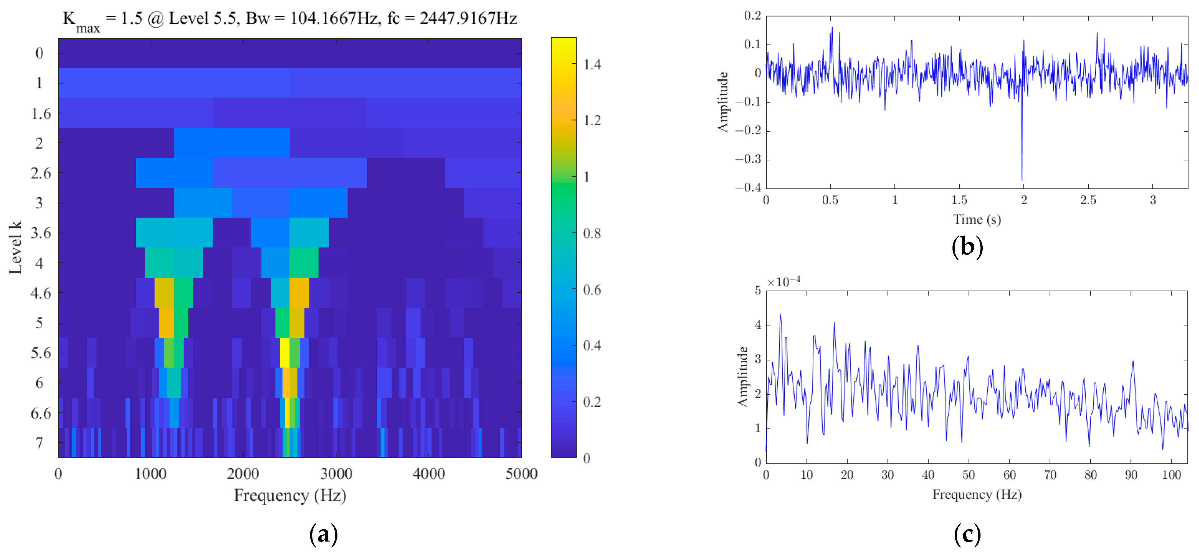
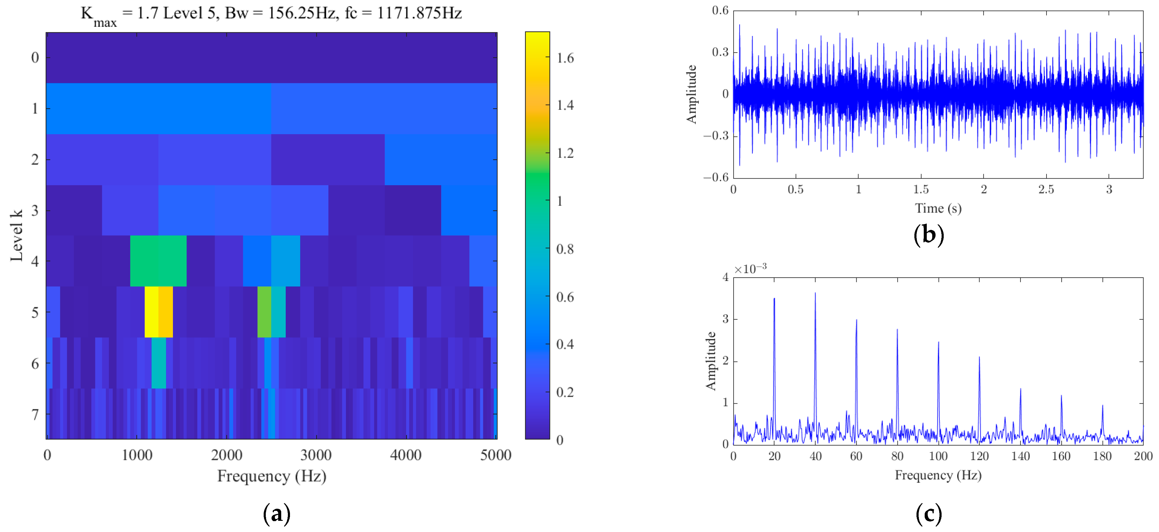
• Select the optimal demodulation band to determine the best frequency band based on the center frequency and bandwidth at the point of maximum kurtosis ($\overline{K}$) value.
• Perform an envelope analysis on the optimal frequency band to extract the fault characteristic frequencies.

The proposed method constructed the FAK through DTCWT and used the squared envelope spectrum (SES) to extract periodic transient signals from the optimal frequency bands identified using the FAK. The SES is widely used in rotating machinery fault diagnosis to highlight fault signal frequency components by emphasizing signal amplitude changes, which makes them more obvious during the spectrum analysis [19,20].

3. Bearing Fault Diagnosis Method Based on the FAK

Bearings are a key component of rotating machinery; their failure leads to equipment performance degradation, reliability reduction, and even serious production accidents. Therefore, effective identification of the bearing health status is key to ensuring safe machinery operation and improving the equipment utilization rate [21]. While a bearing operates, contact between the rolling element and the fault point produces a specific transient impact. This impact is periodic due to the bearing’s rotation. This section describes how FAK and FK algorithms are used to diagnose and compare open bearing data and experimental data, respectively.

Figure 3 shows the cross-sectional schematic diagram of an angular contact ball bearing; its fault characteristic frequency calculation formula is as follows [22]:

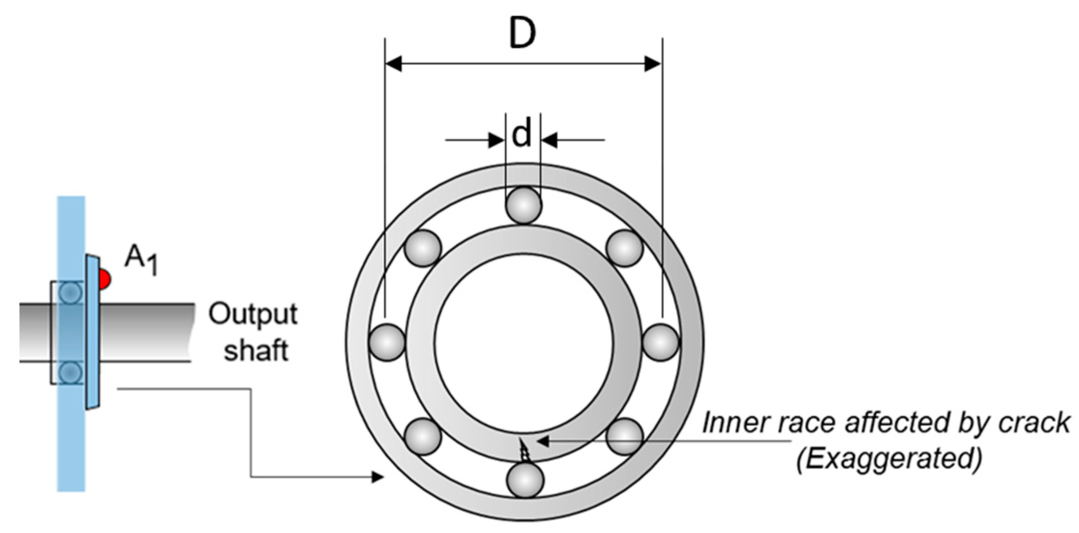
• Ball pass frequency, outer race:

$$f_{BPFO}=\frac{1}{2}{f}_r(1-\frac{d}{D}\cos \alpha )z$$

(11)

• Ball pass frequency, inner race:

$$f_{BPFI}=\frac{1}{2}{f}_r(1+\frac{d}{D}\cos \alpha )z$$

(12)

• Fundamental train frequency, also known as the cage speed:

$$f_{FTF}=\frac{1}{2}{f}_r\left(1-\frac{d}{D}\cos \alpha \right)$$

(13)

• Ball (roller) spin frequency:

$$f_{BSF}=\frac{D}{2d}{f}_r\left[1-{\left(\frac{d}{D}\cos \alpha \right)}^2\right]$$

(14)

In this formula, $f_r$ is the shaft frequency, $D$is the pitch diameter, $d$ is the ball diameter, $\alpha$ is the bearing contact angle and $z$ is the number of rolling elements.

3.1. Simulation Verification

To verify this method’s feasibility, a multi-component simulated signal was constructed for simulation experiments, expressed as follows:

$$s(t)=x(t)+y(t)+z(t)+n(t)$$

(15)

• The signal $x\left(t\right)$ represents a simulated bearing fault signal, which is constructed by superimposing a series of decaying transient sinusoidal waves to model periodic transient impacts caused by faults during the bearing’s operation:

$$x(t)={\displaystyle {\sum }_{k=0}^{100}{\mathrm{e}}^{-80\pi (t-0.05k)}\sin \left[2500\pi (t-0.05k)\right]}$$

(16)

• $y\left(t\right)$ represents an interference signal composed of two low-frequency sinusoidal harmonics:

$$y(t)=0.4\sin (1000\pi t-\pi /4)+0.2\sin (500\pi t)$$

(17)

• $z\left(t\right)$ represents two oscillatory decaying pulse interferences:

$$z(t)=\left\{\begin{array}{ll}{e}^{-20\pi (t-1)}\sin \left[1000\pi (t-1)\right],\hfill & 0\le \mathrm{t}<2\hfill \\ 3e^{-180\pi (t-2)}\sin \left[5000\pi (t-2)\right],\hfill & 2\le \mathrm{t}\hfill \end{array}\right.$$

(18)

• $n\left(t\right)$ represents Gaussian white noise:

$$n(t)=\sqrt{0.5} \mathrm{rand} (t)$$

(19)

Figure 4 shows the time domain waveform and fast Fourier transform (FFT) of the simulated signal, which consists of periodic transient impulses, harmonics, single-pulse interference and Gaussian white noise. Each part’s components are shown in Figure 5 (with a 10,000 Hz sampling frequency and a 33,000 data length).

Figure 6 and Figure 7 show the simulated signal results processed using FK and FAK algorithms, respectively. As shown in Figure 6, the FK algorithm determined the optimal center frequency and bandwidth to be $f_c$ = 2447.916 Hz and $B_w$ = 104.1667 Hz, which was close to the pulse interference fundamental frequency at 2500 Hz. However, as shown in Figure 6b, periodic shocks could not be observed in the band-pass-filtered signal’s time domain. In addition, SES analysis (Figure 6c) failed to accurately extract the periodic transient shock characteristic frequency, indicating that the FK algorithm was affected by pulse interference.

In contrast, the optimal center frequency and bandwidth selected using the FAK algorithm were $f_c$ = 1171.875 Hz and $B_w$ = 156.25 Hz, which was close to the 1250 Hz fundamental frequency of the analog signal’s periodic transient impulse signal. As shown in Figure 7b, the filtered signal clearly displayed an impact waveform with a period of 0.05 s. More importantly, SES analysis was able to accurately extract the characteristic frequencies and harmonics of periodic transient shocks (Figure 7c). The simulation results show that the proposed method could effectively reduce the influence caused by pulse interference, which verified the FAK algorithm’s feasibility and effectiveness.

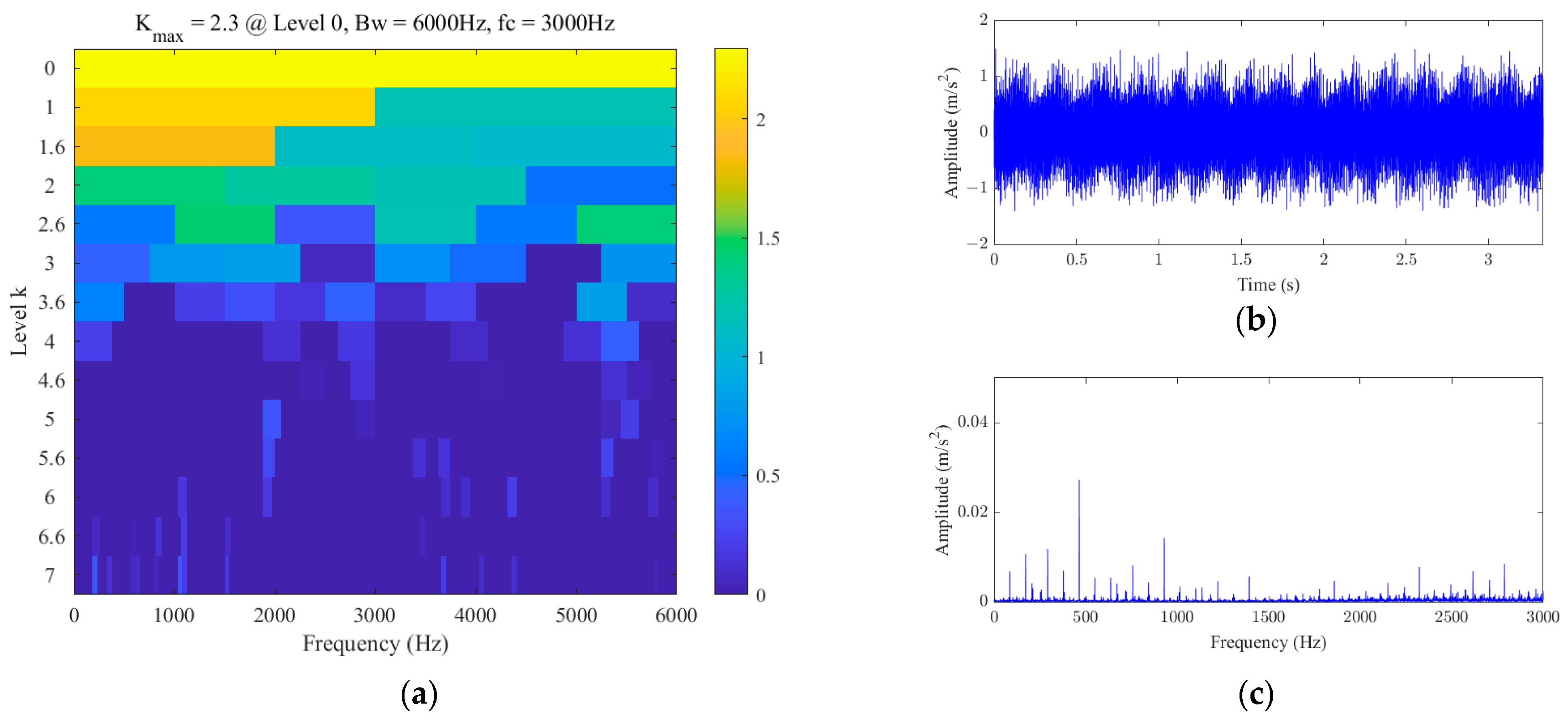
3.2. Open Dataset Test Analysis

3.2.1. Data Source

This section describes the analysis of the public dataset from Case Western Reserve University (CWRU), USA (Figure 8); these data are widely used in the development and evaluation of bearing fault diagnosis technologies. This study analyzed the motor drive-end bearing; detailed parameters are presented in

Table 1. Parameters of 6205-2RS JEM SKF deep-groove ball bearing.

Number of Rolling Elements (z)	Rolling Element Size (d/mm)	Pitch Diameter (D/mm)	Contact Angle ($\mathit{\alpha }/°$)
9	7.94	39.04	0

. An accelerometer was mounted on the bearing housing to collect vibration signals. Test data analyzed included the drive-end bearing’s outer and inner ring faults at a 12 kHz sampling frequency, with a 1730 r/min motor output speed, a 3 HP load, a 0.007 in fault diameter, a 103.36 Hz outer ring fault characteristic frequency and a 156.13 Hz inner ring fault characteristic frequency [23].

3.2.2. Results Analysis

Figure 9 and Figure 10 show the FK and FAK algorithm results, respectively, as applied to the bearings’ outer ring data. Due to the public dataset’s standard nature, both the FK and FAK algorithms selected the same optimal frequency band’s center frequency and bandwidth: $f_c$ = 4500 Hz and $B_w$ = 3000 Hz (Figure 9a and Figure 10a). Similarly, the bearing outer ring’s fault characteristic frequency was successfully extracted from the SES analysis of both methods (Figure 9c and Figure 10c). However, compared with the FAK, the effect was better, the fault characteristic frequency was more prominent and the amplitude was larger. The experimental results of the bearing inner ring are shown in Figure 11 and Figure 12. It can be observed from the figure that the results are consistent with the inner ring experiment. The FAK had a better effect on the fault feature extraction, and the main frequency amplitude of the fault feature frequency extracted by the FAK (Figure 12c) was higher than that of the FK method (Figure 11c). The application to the dataset of Western Reserve University further demonstrated that the FAK algorithm was better than the FK algorithm at the bearing fault diagnosis.

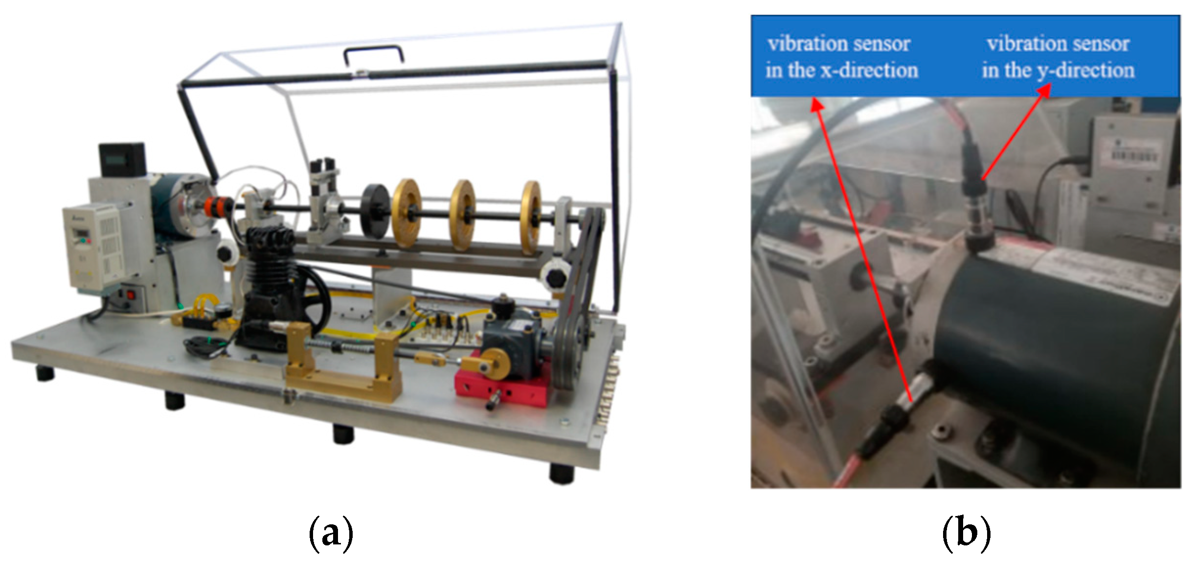
3.3. Laboratory Data Testing Analysis

3.3.1. Experimental Setup

The fault simulation experiments used the Mechanical Fault Simulation (MFS) Testbed produced by Spectra Quest Inc. (Richmond, VA, USA). The test bench was primarily composed of a three-phase asynchronous motor, variable frequency driver, coupling, bearing assembly, rotor assembly, drive shaft, conical gearbox and magnetic brake; its structure is shown in Figure 13a. This experimental platform can be used for rotor dynamics, rotating machinery fault diagnosis, condition monitoring and predictive maintenance experiments. The data acquisition module was a USB-6221 high-speed board card suitable for various data collection and control applications, with a 250 ks/s maximum sampling rate. The vibration accelerometer was a PCB 608A11 piezoelectric sensor, with a 0.5 Hz to 10k Hz frequency range, a 100 m V/g sensitivity and a 350 $\mathsf{\mu }$V broadband resolution.

In this experiment, motor faults were simulated using fault injection, employing a 0.5 horsepower AC motor with an outer ring bearing fault. Detailed bearing parameters can be found in

Table 2. MB ER-10K bearing parameters.

Number of Rolling Elements (z)	Rolling Element Size (d/in)	Pitch Diameter (D/in)	Contact Angle ($\mathit{\alpha }$)
8	0.3125	1.319	0

. The experimental setup used a LabVIEW measurement and control system, with two vibration sensors (in horizontal X- and vertical Y-directions) mounted on the front cover of the motor for data collection, as shown in Figure 13b. The motor’s operating speed was set to 1800 r/min, the magnetic brake gear was set to position 3 and the sampling frequency was set to 12 kHz. Sampling was conducted every 10 s for 1 min, resulting in a total of 12 data segments (6 each in the X- and Y-directions). By analyzing the first three segments of data in the X-direction, we calculated the fault characteristic frequency of the motor bearing outer ring to be 91.56 Hz and conducted envelope analysis on the frequency band with the highest kurtosis value indicated by the FAK. For the validation of the analysis, the remaining three segments of data were used for cross-validation.

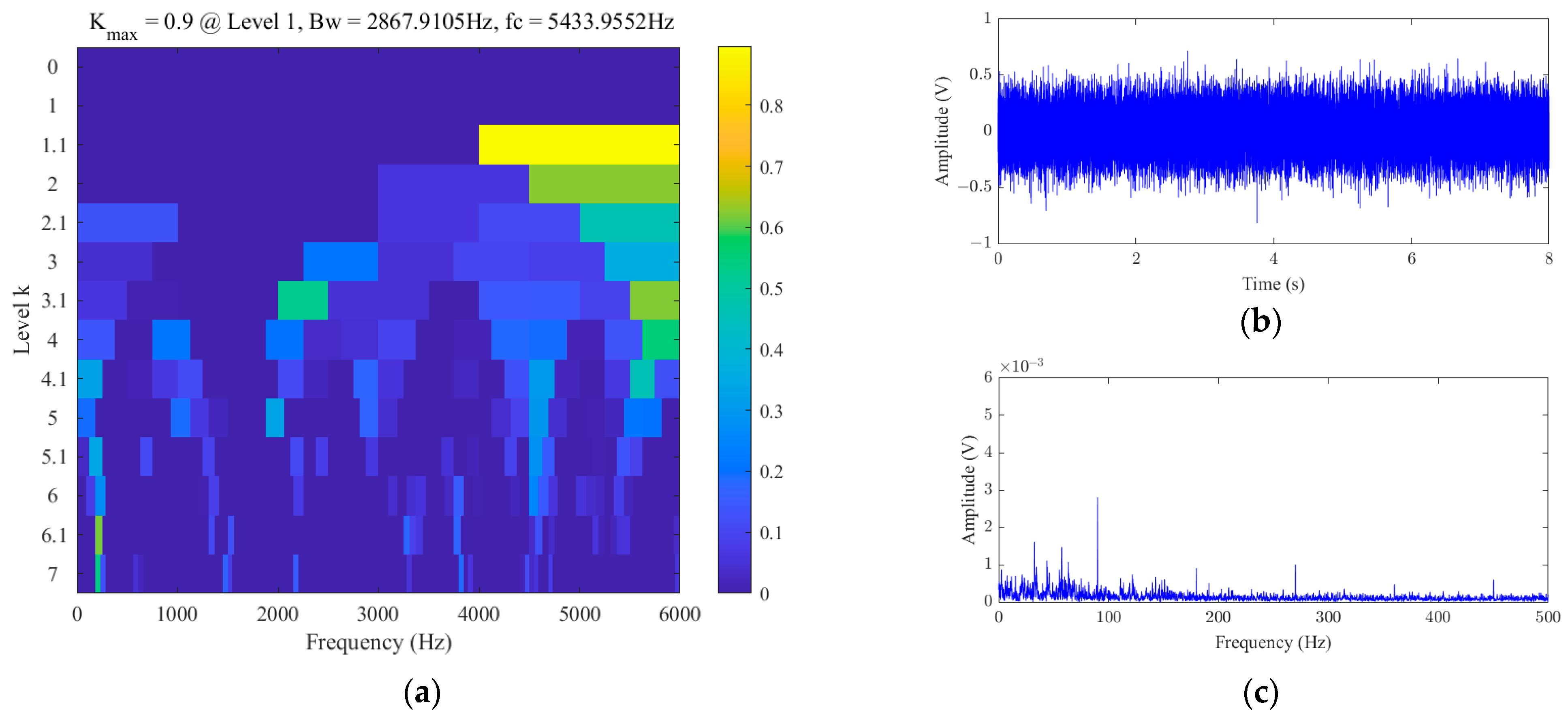
3.3.2. Results Analysis

Figure 14 and Figure 15 show the experimental data results processed using the FK and FAK algorithms, respectively. The optimal center frequency and bandwidth determined using the two methods differed, as shown in Figure 14a and Figure 15a, indicating that the FK algorithm might have been affected by pulse noise. Comparing the SES analyses (Figure 14c and Figure 15c) showed that the FAK (Figure 15c) was more accurate in extracting the characteristic frequencies and harmonics of periodic transient shocks. This further confirmed this method’s advantages and wide applicability in bearing fault diagnosis.

4. Application of Deep Learning in Fault Diagnosis

4.1. Introduction to Convolutional Neural Networks

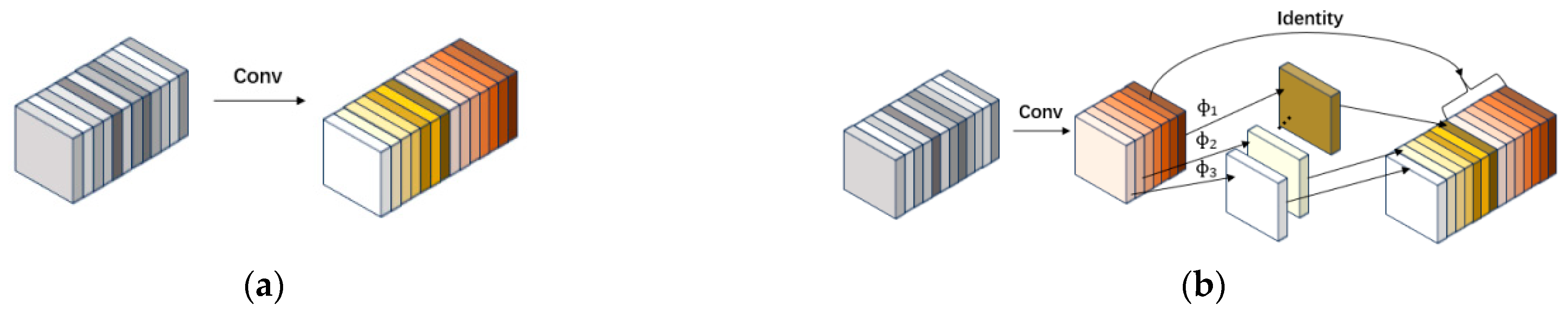
With significant improvements in computational power and substantial increases in data volume, deep learning, especially CNNs, has become a popular research direction in the fault diagnosis field [24]. CNNs can learn fault features from complex sensor data and automatically identify different types of mechanical faults. This method greatly reduces the dependence on expert knowledge compared with traditional diagnostic techniques and improves fault diagnosis accuracy and efficiency. With the diversification and complexity of application scenarios, traditional CNN models might experience slow computational speed and high memory usage, especially in resource-limited environments [25,26,27]. To address this, researchers have developed various high-efficiency, compact and lightweight models, including the GhostNet model, to enhance the models’ robustness and processing speeds [28].

4.2. GhostNet Model

GhostNet is a lightweight convolutional neural network that was proposed in 2020 and designed to provide efficient computational performance while reducing the model size. Its core is the “Ghost Module”, which first generates fewer “eigenfeature graphs” compared with traditional full convolution, and then obtains “Ghost feature graphs” through low-cost linear transformations. Finally, the eigenfeature map and Ghost feature map are combined to obtain the same number of feature maps at a lower computational cost [29]. Compared with current mainstream convolution operations, the Ghost Module has the following advantages [30,31]:

• Model compression: As the Ghost Module performs real convolution operations on only a subset of channels, it requires significantly fewer parameters than traditional convolutions. This design strategy reduces the model’s storage requirements and makes it more suitable for resource-limited environments.
• Design flexibility: the Ghost Module introduces a new hyperparameter, namely, the ratio of output channels that undergo actual convolution, offering researchers the possibility to adjust the balance between computation and performance, facilitating optimization according to actual application needs.
• High integrability: the Ghost Module is highly adaptable and can be used as a plug-and-play module to upgrade existing convolutional neural networks for various image classification tasks.
• For a typical convolutional layer, as shown in Figure 16a, its computational process can be represented as

$$Y=X\times f+b$$

(20)

In this formula, $X\in R^{c\times h\times w}$ represents the given input data, where $h$ and $w$ are the height and width of the input data, respectively; $c$ is the number of channels; $\times$ denotes the convolution operation; $f\in R^{c\times k\times k\times n}$ is the convolution kernel of the layer, where $k\times k$ is the kernel size; $b$ is the bias term; and $Y{\in R}^{h^{\prime }\times w^{\prime }\times n}$ is the output feature map, where $h^{\prime }$ and $w^{\prime }$ are the feature map’s height and width, respectively, and $n$ is the number of output channels.

The Ghost Module’s convolutional calculation process is shown in Figure 16b. In the first step, fewer convolutional kernels were used to generate an eigenmap; in the second step, a series of linear transformations were performed on each eigenmap to obtain the same number of output eigenmaps as an ordinary convolutional layer would.

The first step’s standard convolutional computation process is

$$Y^{\prime }=X\times f^{\prime }$$

(21)

In this formula, $X\in R^{c\times h\times w}$ represents the given input data; $f^{\prime }\in R^{c\times k\times k\times m}$ is the convolution kernel used $(m\le n)$; $Y^{\prime }\in R^{h^{\prime }\times w^{\prime }\times m}$ is the output intermediate feature map, where $m$ is the number of output channels; and for simplicity, the bias term was set to 0.

The second step’s linear transformation computational process is

$$y_{ij}={\Phi }_{ij}\left(y_i^{\prime }\right), \forall i=1,\dots ,m j=1,\dots ,s$$

(22)

In this formula, $y_i^{\prime }$ is the ith feature map in $Y^{\prime }$ and ${\Phi }_{ij}$ is the function of the jth linear transformation of $y_i^{\prime }$. For each $y_i^{\prime }$, there are $s$ linear transformations, one of which is an identity mapping (usually ${\Phi }_{is}$); the remaining $s-1$ are different linear operations, which are typically simple convolution calculations.

Through the above transformation, we can obtain $m·s=n$ feature graphs $Y^{″}=\left[y_{11},y_{12}, \dots ,y_{ms}\right]$ as Ghost Module output data. In this way, the same number of output feature maps as produced by ordinary convolutional layers can be generated, which can then be integrated into the existing designed neural network structure to effectively reduce the computational cost. Specifically, the Ghost Module has $m·(s-1)$ linear transformations and $m$ identity mapping operations, with a $d\times d$ convolution kernel size for each linear operation. Each linear operation can theoretically have a different convolution kernel, but given the efficiency of the CPU and GPU, the same-sized convolution kernel is usually used in a Ghost Module.

A Ghost Module’s theoretical speed-up ratio compared with standard convolution is

$$r_s=\frac{n·h^{\prime }·w^{\prime }·c·k·k}{\frac{n}{s}·h^{\prime }·w^{\prime }·c·k·k+\left(s-1\right)·\frac{n}{s}·h^{\prime }·w^{\prime }·d·d}=\frac{c·k·k}{\frac{1}{s}·c·k·k+\frac{s-1}{s}d·d}\approx \frac{s·c}{s+c-1}\approx s$$

(23)

The theoretical parameter compression ratio is

$$r_c=\frac{n·c·k·k}{\frac{n}{s}·c·k·k+\left(s-1\right)·\frac{n}{s}·d·d}\approx \frac{s·c}{s+c-1}\approx s$$

(24)

In this formula, $d\times d$ and $k\times k$ are of similar magnitude and s ≪ c. According to the research in [32], when$d=3$ and $s=2$, the Ghost Module exhibits better performance compared with other values.

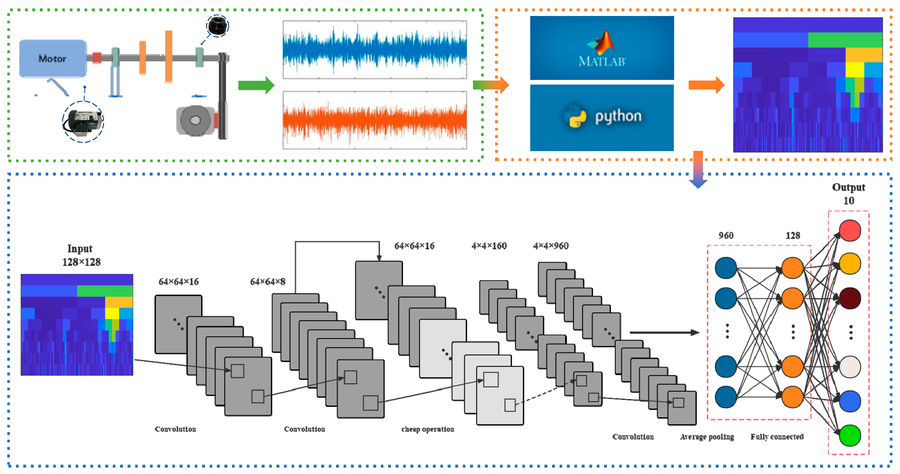
5. Intelligent Fault Diagnosis Method Based on FAK-GhostNet

5.1. Method Overview

Currently, many CNN-based fault diagnosis systems use it as both a feature extractor and a classifier. However, the collected signal often contains a variety of components, which may be caused by different mechanical faults or operating conditions, and key fault features are often masked by background noise. This makes the direct input of the original signal into the deep learning model potentially less accurate for diagnosis [33]. CNNs are highly effective deep learning architectures that are widely used in image classification and computer vision, often requiring two-dimensional images as input. Therefore, this paper proposes a feature extraction and diagnosis method for periodic transient shock faults based on FAK-GhostNet. As shown in Figure 17, the method mainly includes four parts: data acquisition, feature extraction, fault diagnosis and classification.

First, the experimental environment is set up, and the bearing vibration signal is collected. The FAK algorithm is then used to convert the one-dimensional signal into a two-dimensional feature graph. This step is critical because it allows us to efficiently express and analyze signals that would otherwise be difficult to parse in two-dimensional space. The converted 2D feature map is then analyzed using the GhostNet model to accurately identify and classify different fault types in bearings. As shown in Section 2, we verified the effectiveness of the FAK algorithm through a series of experiments. Compared with the traditional FK method, FAK showed remarkable advantages in eliminating pulse noise interference and significantly improved the ability to extract fault features. At the same time, combined with the lightweight GhostNet model, our approach greatly improved the processing efficiency while ensuring diagnostic accuracy.

5.2. Rolling Bearing Fault Diagnosis Experiment

5.2.1. Experimental Setup

The bearing fault simulation experiment used the Mechanical Fault Simulation (MFS) Testbed with the M-BFK-3/4 bearing fault kit. The kit includes bearings with inner ring faults, outer ring faults, rolling element faults and composite faults (comprising the previous three types). Specific bearing parameters are listed in

Table 3. MB ER-12K bearing parameters.

Number of Rolling Elements (z)	Rolling Element Size (d/in)	Pitch Diameter (D/in)	Contact Angle ($\mathit{\alpha }/°$)
8	0.3125	1.318	0

. The motor’s output speed was set to 1800 r/min, the force brake was set to position 3, and the sampling frequency was 12 kHz. In each experiment, only the faulty bearing was replaced while the motor and other conditions remained unchanged. Sampling was conducted every 10 s for 2 min, thus obtaining six segments of data in both the X- and Y-directions for each type of fault. Since the bearing on the left side of the motor output shaft might be significantly affected by the noise and vibration of the motor itself, only sensor data from the bearing on the right side was considered. This setup was intended to ensure the accuracy of the data, making the vibration signals more truly reflect the state of the bearing faults rather than the operation of the motor (Figure 18). This experimental configuration is consistent with the previous motor bearing fault simulation experiments.

In this study, the seven-level FAK of vibration signals under five different bearing states was calculated, including an inner ring fault, outer ring fault, rolling element fault, compound fault (combination of an inner ring and outer ring fault) and normal state, to show the vibration characteristics of different fault types, and the obtained FAK image size was 128 × 128. In the experiment, 5000 samples (1000 instances of each state) were randomly assigned to the training set, the validation set, and the test set, in proportions of 80%, 10%, and 10%. This allocation was designed to ensure that the model was adequately trained on all types of data while retaining enough data for validation and testing. As shown in Figure 19, FAK images of different bearing states presented unique patterns, providing rich feature information for the GhostNet model.

As shown in

Table 4. GhostNet architecture.

Input	Output	Operator	#exp	SE	Stride
128 × 128 × 3	64 × 64 × 16	Conv2d 3 × 3	-	-	2
64 × 64 × 16	64 × 64 × 16	G-bneck	16	-	1
64 × 64 × 16	32 × 32 × 24	G-bneck	48	-	2
32 × 32 ×24	32 × 32 × 24	G-bneck	72	-	1
32 × 32 × 24	16 × 16 × 40	G-bneck	72	1	2
16 × 16 × 40	16 × 16 × 40	G-bneck	120	1	1
16 × 16 × 40	8 × 8 × 80	G-bneck	240	-	2
8 × 8 × 80	8 × 8 × 80	G-bneck	200	-	1
8 × 8 × 80	8 × 8 × 80	G-bneck	184	-	1
8 × 8 × 80	8 × 8 × 80	G-bneck	184	-	1
8 × 8 × 80	8 × 8 × 112	G-bneck	480	1	1
8 × 8 × 112	8 × 8 × 112	G-bneck	672	1	1
8 × 8 × 112	4 × 4 × 160	G-bneck	672	1	2
4 × 4 × 160	4 × 4 × 160	G-bneck	960	-	1
4 × 4 × 160	4 × 4 × 160	G-bneck	960	1	1
4 × 4 × 160	4 × 4 × 160	G-bneck	960	-	1
4 × 4 × 160	4 × 4 × 160	G-bneck	960	1	1
4 × 4 × 160	4 × 4 × 960	Conv2d 1 × 1	-	-	1
4 × 4 × 960	1 × 1 × 960	AvgPool4 × 4	-	-	-
1 × 1 × 960	1 × 1 × 128	FC	-	-	-
1 × 1 × 128	1 × 1 × 5	FC	-	-	-

, the first layer of the GhostNet network is the standard convolution layer, which contains 16 convolution cores and is mainly used to extract primary features. Subsequent layers 2 through 17 contain a series of Ghost Bottleneck (G-bneck) structures, which are responsible for further extracting and refining higher-level features. At the end of the network, a global average pooling layer and a fully connected layer are used to integrate these features to complete the final classification task. When the model is trained, the batch size is set to 32 to balance the memory usage and training efficiency. A total of five training cycles were performed, each consisting of 125 iterations, which was a setup designed to optimize the model performance while avoiding overfitting. In order to reflect the advantages of lightweight convolutional neural network GhostNet, ResNet18 and lightweight network MobileNetV2 are also introduced for comparison.

ResNet18 is a classic deep convolutional neural network model that is notable for introducing the concept of residual blocks to address the issues of vanishing and exploding gradients in deep convolutional networks. These residual blocks allow for information to be transmitted across layers via “skip connections”, effectively solving the vanishing gradient problem in deep networks. ResNet18 has been widely applied in various image recognition tasks, including image classification, object detection and image segmentation [34]. Compared with ResNet18, GhostNet significantly reduces the computational demands and model size using an efficient method of feature map generation. This design allows GhostNet to excel in edge computing and mobile devices while maintaining accuracy comparable with ResNet18.

MobileNetV2 is a lightweight deep learning architecture designed specifically for computer vision tasks on mobile and embedded devices. It is part of the MobileNet series developed by Google’s research team. MobileNetV2 is based on a structure known as depthwise separable convolutions, which decomposes standard convolutions into depthwise and pointwise convolutions. This design reduces the model’s parameter count and computational load while maintaining strong performance [35]. Both MobileNetV2 and GhostNet are designed to provide efficient deep learning solutions on mobile and edge devices. However, as MobileNetV2 was introduced earlier, its performance and efficiency are slightly inferior to those of GhostNet.

5.2.2. Results Analysis

Table 5. Models’ performance comparison.

Model	Acc. (%)	MFLOPs	Params/106	MemR + W(MB)	Images/s
FK–GhostNet	0.9848	49.51	2.79	36.5	82
FAK–GhostNet	0.9902	49.51	2.79	36.5	85
FAK–ResNet18	0.9930	594.58	11.18	59.77	59
FAK-MobileNetV2	0.9820	104.16	2.23	57.11	57

summarizes the performance indicators of the four models in the task of bearing fault diagnosis, namely, FK-GhostNet, FAK-GhostNet, FAK-ResNet18 and FAK-MobileNetV2, with Figure 20 presenting the confusion matrices of these methods. This study evaluated each model’s accuracy, computational complexity (MFLOPs), number of parameters (params), memory requirements (MemR+W) and processing speed (images/second). In terms of accuracy, FAK-ResNet18 led with 99.3%, followed by FAK-GhostNet at 99.02%, FAK-MobileNetV2 at 98.90% and FK-GhostNet at 98.48%. This indicates that the FAK method had a significant advantage over FK in eliminating noise interference, as such noise often affected the extraction of fault features and reduced the model accuracy. It also validated the effectiveness of the FAK as a feature extraction method in accurately identifying bearing faults. In terms of computational resource consumption, the GhostNet architecture showed higher efficiency compared with MobileNetV2, with approximately half the computational complexity and memory requirements of MobileNetV2. Compared with FAK-ResNet18, GhostNet’s computational complexity was only about a tenth, with about a fifth of the number of parameters and half the memory requirement. These metrics indicate that FAK-GhostNet significantly reduced the demand for computational resources while maintaining high accuracy.

Overall, FAK-GhostNet significantly reduced the consumption of computational resources while maintaining accuracy comparable with traditional CNNs. Compared with the typical lightweight network MobileNetV2, it did not compromise on accuracy and had a smaller model size and lower computational demands. The FAK-GhostNet model stood out among these four bearing fault diagnosis methods due to its balance between accuracy and computational efficiency. It demonstrates potential for application in resource-constrained environments and offers an efficient and reliable solution for real-time bearing fault monitoring.

6. Discussion

The FAK-GhostNet method provides a highly efficient and accurate new approach for diagnosing periodic transient impact faults. It combines advanced signal processing techniques with deep learning. This study improved the original FK (frequency kurtosis) algorithm by replacing its filters with DTCWPT (dual-tree complex wavelet packet transform) and integrating the concept of frequency domain averaging into the algorithm design. This enhancement not only improves the algorithm’s ability to suppress high kurtosis value pulse noise but also enhances the efficiency and accuracy of fault feature extraction. As shown in the second section, the effectiveness of this method was validated using simulation signals, namely, the publicly available bearing dataset from Case Western Reserve University, and experimental results from the Mechanical Fault Simulation Testbed.

Next, this study input the kurtosis graph extracted by the FAK algorithm as a two-dimensional feature into the GhostNet model, successfully solving the challenges of rolling bearing fault diagnosis and classification. Comparative analysis, especially based on the bearing data from the Mechanical Fault Simulation Testbed, showed that FAK-GhostNet outperformed other fault diagnosis models in the feature extraction and diagnosis of periodic transient impact faults.

However, the FAK-GhostNet method also has potential limitations. On the one hand, the computational complexity introduced by the DTCWPT component may affect the real-time application performance of the algorithm. On the other hand, compared with the traditional FK algorithm, DTCWPT’s more refined frequency band division and its binary tree structure (equivalent to 0.5) may not be as flexible as the FK algorithm’s ternary tree structure (0.333) in some cases. Additionally, while this method effectively suppresses high kurtosis value pulse noise, it may overlook important fault indicators in certain situations. Therefore, finding a balance between noise reduction and preserving fault features is a key direction for future research.

7. Conclusions

The FAK-GhostNet method provides a highly efficient and accurate new approach for diagnosing periodic transient impact faults. It combines advanced signal processing techniques with deep learning models, demonstrating significant performance advantages. This method can suppress the impact of non-Gaussian noise in the signal on the kurtosis graph, enhancing the accuracy of the filter center frequency and bandwidth selection in envelope analysis, and can accurately extract the characteristic frequencies of rolling bearing faults. In this study, the 0.5-binary tree kurtosis graph generated using the FAK algorithm was used as input, solving the problem of representing one-dimensional mechanical signals in a two-dimensional format. This representation provides an efficient data input format for the lightweight convolutional neural network GhostNet, enabling it to extract high-quality discriminative features from these graphs. Moreover, GhostNet showed a high level of generalization ability when classifying unknown samples. The experimental results indicate that this method could achieve high-precision intelligent fault diagnosis of rolling element bearings under various rotational speeds. Furthermore, this study also found that the FAK graph of mechanical equipment vibration signals could serve as an input image for the CNN structure, without the need for significant modifications to the internal structure of the CNN, demonstrating the method’s wide applicability and flexibility in the field of mechanical fault diagnosis.

References

1. Wang, C.Y.; Jiang, W.L.; Yue, Y.; Zhang, S.Q. Research on Prediction Method of Gear Pump Remaining Useful Life Based on DCAE and Bi-LSTM. Symmetry 2022, 14, 1111. [Google Scholar] [CrossRef]
2. Dwyer, R. Use of the Kurtosis Statistic in the Frequency Domain as an Aid in Detecting Random Signals. IEEE J. Ocean. Eng. 1984, 9, 85–92. [Google Scholar] [CrossRef]
3. Lei, Y.; Lin, J.; He, Z.; Zi, Y. Application of an Improved Kurtogram Method for Fault Diagnosis of Rolling Element Bearings. Mech. Syst. Signal Process. 2011, 25, 1738–1749. [Google Scholar] [CrossRef]
4. Zhang, Y.; Randall, R.B. Rolling Element Bearing Fault Diagnosis Based on the Combination of Genetic Algorithms and Fast Kurtogram. Mech. Syst. Signal Process. 2009, 23, 1509–1517. [Google Scholar] [CrossRef]
5. Chen, B.; Zhang, Z.; Zi, Y.; He, Z.; Sun, C. Detecting of Transient Vibration Signatures Using an Improved Fast Spatial–Spectral Ensemble Kurtosis Kurtogram and Its Applications to Mechanical Signature Analysis of Short Duration Data from Rotating Machinery. Mech. Syst. Signal Process. 2013, 40, 1–37. [Google Scholar] [CrossRef]
6. Li, B.; Xu, X.; Tan, H.; Shi, P.; Qiao, Z. Cyclogram: An Effective Method for Selecting Frequency Bands for Fault Diagnosis of Rolling Element Bearings. Meas. Sci. Technol. 2023, 34, 094003. [Google Scholar] [CrossRef]
7. Dai, S.-C.; Guo, Y.; Wu, X.; Na, J. Improvement of fast spectral kurtograph algorithm based on subband spectral kurtosis average. Vib. Shock 2015, 34, 98–102. [Google Scholar]
8. Wang, L.; Liu, Z.; Cao, H.; Zhang, X. Subband Averaging Kurtogram with Dual-Tree Complex Wavelet Packet Transform for Rotating Machinery Fault Diagnosis. Mech. Syst. Signal Process. 2020, 142, 106755. [Google Scholar] [CrossRef]
9. Tian, Z.; Wong, L.; Safaei, N. A Neural Network Approach for Remaining Useful Life Prediction Utilizing Both Failure and Suspension Histories. Mech. Syst. Signal Process. 2010, 24, 1542–1555. [Google Scholar] [CrossRef]
10. Wang, J.; Yu, L.-C.; Lai, K.R.; Zhang, X. Dimensional Sentiment Analysis Using a Regional CNN-LSTM Model. In Proceedings of the 54th Annual Meeting of the Association for Computational Linguistics (Volume 2: Short Papers), Berlin, Germany, 7–12 August 2016; Erk, K., Smith, N.A., Eds.; Association for Computational Linguistics: Berlin, Germany, 2016; pp. 225–230. [Google Scholar]
11. Huang, C.; Kong, C.; Lucey, S. CNNs Are Globally Optimal Given Multi-Layer Support. arXiv 2017, arXiv:1712.02501. [Google Scholar]
12. Chu, D.C.; Humphrey, M. Mobile OGSI.NET: Grid Computing on Mobile Devices. In Proceedings of the Fifth IEEE/ACM International Workshop on Grid Computing, Pittsburgh, PA, USA, 8 November 2004; pp. 182–191. [Google Scholar]
13. Paul, R.R.; Valgenti, V.C.; Kim, M.S. Real-Time Netshuffle: Graph Distortion for on-Line Anonymization. In Proceedings of the 2011 19th IEEE International Conference on Network Protocols, Vancouver, BC, Canada, 17–20 October 2011; pp. 133–134. [Google Scholar]
14. Gholami, A.; Kwon, K.; Wu, B.; Tai, Z.; Yue, X.; Jin, P.; Zhao, S.; Keutzer, K. SqueezeNext: Hardware-Aware Neural Network Design. In Proceedings of the 2018 IEEE/CVF Conference on Computer Vision and Pattern Recognition Workshops (CVPRW), Salt Lake City, UT, USA, 18–22 June 2018; pp. 1719–171909. [Google Scholar]
15. Cao, M.; Fu, H.; Zhu, J.; Cai, C. Lightweight Tea Bud Recognition Network Integrating GhostNet and YOLOv5. Math. Biosci. Eng. 2022, 19, 12897–12914. [Google Scholar] [CrossRef]
16. Antoni, J. The Spectral Kurtosis: A Useful Tool for Characterising Non-Stationary Signals. Mech. Syst. Signal Process. 2006, 20, 282–307. [Google Scholar] [CrossRef]
17. Antoni, J. Fast Computation of the Kurtogram for the Detection of Transient Faults. Mech. Syst. Signal Process. 2007, 21, 108–124. [Google Scholar] [CrossRef]
18. Borghesani, P.; Ricci, R.; Chatterton, S.; Pennacchi, P. A New Procedure for Using Envelope Analysis for Rolling Element Bearing Diagnostics in Variable Operating Conditions. Mech. Syst. Signal Process. 2013, 38, 23–35. [Google Scholar] [CrossRef]
19. Randall, R.B.; Antoni, J.; Chobsaard, S. The relationship between spectral correlation and envelope analysis in the diagnostics of bearing faults and other cyclostationary machine signals. Mech. Syst. Signal Process. 2001, 15, 945–962. [Google Scholar] [CrossRef]
20. Yu, L.; Hai, L. Fault diagnosis method of rolling bearings with different specifications based on federated model migration. Vib. Shock 2023, 42, 184–192. [Google Scholar]
21. Zhi, C.; Xu, C. Application of deep learning in equipment failure prediction and health management. Chin. J. Sci. Instrum. 2020, 40, 206–226. [Google Scholar]
22. Randall, R.B. Rolling Element Bearing Diagnostics—A Tutorial. Mech. Syst. Signal Process. 2011, 25, 485–520. [Google Scholar] [CrossRef]
23. Smith, W.A.; Randall, R.B. Rolling Element Bearing Diagnostics Using the Case Western Reserve University Data: A Benchmark Study. Mech. Syst. Signal Process. 2015, 64–65, 100–131. [Google Scholar] [CrossRef]
24. Liu, H.; Ma, R.; Li, D.; Yan, L.; Ma, Z. Machinery Fault Diagnosis Based on Deep Learning for Time Series Analysis and Knowledge Graphs. J. Signal Process. Syst. 2021, 93, 1433–1455. [Google Scholar] [CrossRef]
25. Shao, S.; Zhang, S.; Jiang, W.; Li, Z. Study on the Health Condition Monitoring Method of Hydraulic Pump Based on Convolutional Neural Network. In Proceedings of the 2020 12th International Conference on Measuring Technology and Mechatronics Automation (ICMTMA), Phuket, Thailand, 28–29 February 2020; pp. 149–153. [Google Scholar]
26. Ming, D.; Bao, W. Fault diagnosis of hydraulic pump based on empirical wavelet decomposition and convolutional neural network. Chin. Hydraul. Pneum. 2020, 1, 163–170. [Google Scholar]
27. Khan, A.; Sohail, A.; Zahoora, U.; Qureshi, A.S. A Survey of the Recent Architectures of Deep Convolutional Neural Networks. Artif. Intell. Rev. 2020, 53, 5455–5516. [Google Scholar] [CrossRef]
28. Zhou, Y.; Chen, S.; Wang, Y.; Huan, W. Review of Research on Lightweight Convolutional Neural Networks. In Proceedings of the 2020 IEEE 5th Information Technology and Mechatronics Engineering Conference (ITOEC), Chongqing, China, 12–14 June 2020; pp. 1713–1720. [Google Scholar]
29. Han, K.; Wang, Y.; Tian, Q.; Guo, J.; Xu, C.; Xu, C. GhostNet: More Features from Cheap Operations. In Proceedings of the 2020 IEEE/CVF Conference on Computer Vision and Pattern Recognition (CVPR), Seattle, WA, USA, 13–19 June 2020; pp. 1577–1586. [Google Scholar]
30. Lang, X.; Han, F. MFL Image Recognition Method of Pipeline Corrosion Defects Based on Multilayer Feature Fusion Multiscale GhostNet. IEEE Trans. Instrum. Meas. 2022, 71, 1–8. [Google Scholar] [CrossRef]
31. Li, S.; Sultonov, F.; Tursunboev, J.; Park, J.-H.; Yun, S.; Kang, J.-M. Ghostformer: A GhostNet-Based Two-Stage Transformer for Small Object Detection. Sensors 2022, 22, 6939. [Google Scholar] [CrossRef] [PubMed]
32. Chi, J.; Guo, S.; Zhang, H.; Shan, Y. L-GhostNet: Extract Better Quality Features. IEEE Access 2023, 11, 2361–2374. [Google Scholar] [CrossRef]
33. Udmale, S.S.; Patil, S.S.; Phalle, V.M.; Singh, S.K. A Bearing Vibration Data Analysis Based on Spectral Kurtosis and ConvNet. Soft Comput. 2019, 23, 9341–9359. [Google Scholar] [CrossRef]
34. Huang, B.; Liu, J.; Zhang, Q.; Liu, K.; Li, K.; Liao, X. Identification and Classification of Aluminum Scrap Grades Based on the Resnet18 Model. Appl. Sci. 2022, 12, 11133. [Google Scholar] [CrossRef]
35. Sandler, M.; Howard, A.; Zhu, M.; Zhmoginov, A.; Chen, L.-C. MobileNetV2: Inverted Residuals and Linear Bottlenecks. In Proceedings of the 2018 IEEE/CVF Conference on Computer Vision and Pattern Recognition, Salt Lake City, UT, USA, 18–23 June 2018; pp. 4510–4520. [Google Scholar]
Figure 1. FK algorithm diagrams: (a) low-pass/high-pass filters and (b) fast computation of the kurtogram by means of an arborescent filter bank structure.
Processes 12 00287 g001
Figure 2. Kurtosis of signal: (a) single pulse interference and (b) periodic transient impact signal.
Processes 12 00287 g002
Figure 3. Rolling bearing section diagram.
Processes 12 00287 g003
Figure 4. Simulated signal s ( t ) : (a) time domain waveform and (b) fast Fourier transform spectrum.
Processes 12 00287 g004
Figure 5. Simulated signal components: (a) periodic transient impulse signal x ( t ) , (b) harmonic signal y ( t ) , (c) single-pulse interference z ( t ) and (d) Gaussian white noise n ( t ) .
Processes 12 00287 g005
Figure 6. FK algorithm processing results: (a) kurtogram, (b) filtered signal and (c) SES.
Processes 12 00287 g006
Figure 7. FAK algorithm processing results: (a) kurtogram, (b) filtered signal and (c) SES.
Processes 12 00287 g007
Figure 8. Case Western Reserve University (CWRU) bearing fault test bench.
Processes 12 00287 g008
Figure 9. FK algorithm processing results for outer race fault: (a) kurtogram, (b) filtered signal and (c) SES.
Processes 12 00287 g009
Figure 10. FAK algorithm processing results for outer race fault: (a) kurtogram, (b) filtered signal and (c) SES.
Processes 12 00287 g010
Figure 11. FK algorithm processing results for inner race fault: (a) kurtogram, (b) filtered signal and (c) SES.
Processes 12 00287 g011
Figure 12. FAK algorithm processing results for inner race fault: (a) kurtogram, (b) filtered signal and (c) SES.
Processes 12 00287 g012
Figure 13. SQI fault simulation test bench: (a) test bench, (b) sensor position installation.
Processes 12 00287 g013
Figure 14. FK algorithm processing results for inner race fault: (a) kurtogram, (b) filtered signal and (c) SES.
Processes 12 00287 g014
Figure 15. FAK algorithm processing results for motor bearing inner race fault: (a) kurtogram, (b) filtered signal and (c) SES.
Processes 12 00287 g015
Figure 16. Convolution computation diagram: (a) classical convolution and (b) Ghost Module.
Processes 12 00287 g016
Figure 17. FAK-GhostNet fault diagnosis flowchart.
Processes 12 00287 g017
Figure 18. Sensor layout diagram.
Processes 12 00287 g018
Figure 19. FAK of various rolling-element bearing states: (a) normal, (b) inner, (c) outer, (d) roller and (e) compound.
Processes 12 00287 g019
Figure 20. Confusion matrices: (a) FK–GhostNet, (b) FAK–GhostNet, (c) FAK–ResNet18 and (d) FAK–MobileNetV2.
Processes 12 00287 g020