Health Management of Bearings Using Adaptive Parametric VMD and Flying Squirrel Search Algorithms to Optimize SVM

Abstract

Bearing, as one of the core parts of rotating machinery, has a running state which is related to the overall operation of the system. Due to the bearing structure and its complex operating environment, running condition monitoring and fault diagnosis is always a key problem in the field of bearing health management, which is of great significance for bearing maintenance and equipment reliability and safety. In view of the difficulty in parameter selection and poor feature extraction ability of variational mode decomposition (VMD) in existing feature extraction, this paper uses the flying squirrel search algorithm (SSA) to optimize the parametric of decomposition layer k and penalty factor α in VMD, and forms an adaptive VMD signal decomposition method. To solve the problem of high dimensionality and long extraction time of multi-domain fault feature set, kernel principal component analysis (KPCA) is used to reduce feature dimensionality. Then, the processed features are input into the support vector machine (SVM) for fault diagnosis and classification, and the parameter optimization ability of SSA is used again to build the SSA-SVM fault diagnosis model. To evaluate the running state of bearings, an alarm threshold method based on the root mean square value calculated by cosine similarity and 3σ is proposed to divide samples of different health states. Finally, the method constructed in this paper is compared with other methods by using simulation and experimental data sets, and the running condition monitoring and fault diagnosis of rolling bearings are successfully realized, which shows the superiority and effectiveness of the method proposed in this paper.

1. Introduction

As a crucial component of rotating mechanical equipment, working in a long-term operating state, there will be a tendency to degradation, which has a significant impact on the overall performance of the mechanical system [1,2]. Consequently, the health management of bearings directly impacts equipment performance, service life, production capacity, and operational efficiency of the entire manufacturing system.

Health management research primarily focuses on fault diagnosis and health state assessment. However, the vibration signals used as input for bearing condition monitoring models are often nonlinear, non-smooth, and characterized by weak fault signals and significant background noise, making it challenging to extract effective fault characteristics [3,4,5]. In terms of optimal demodulation frequency band (ODFB), Wang et al. [6] proposed an ergodic index enhanced graph (TIEgram), which uses the ergodic segmentation model to transfer the original signal into the frequency domain to solve the problem that a single indicator cannot detect different signals. In recent years, empirical mode decomposition (EMD) has been widely applied in fault feature extraction [7]. Aggarwal et al. [8] used EMD to process current signals and carried out feature extraction for 10 kinds of shunt faults. However, EMD lacks theoretical basis, and there are some deficiencies such as mode aliasing of adjacent mode components and end effects of data divergence at both ends of the envelope [9]. In this regard, Dragomiretskiy et al. [10] proposed variational mode decomposition (VMD) to avoid EMD mode aliasing and end effects. However, VMD also has defects and deficiencies, and its decomposition effect is closely related to the selection of model parameters [11], involving decomposition layers k and penalty factor α. Wu et al. [12] used the spectrum trend algorithm to find the resonance band boundary and determine the relevant parameters of the VMD algorithm, but the obtained parameter values need to be returned to the model for re-input, which increases the complexity of the algorithm. Wang et al. [13] constructed a method to reduce the overlap index of adjacent modes to determine the number of decomposition layers in VMD, but ignored the problem of optimization of penalty factor parameters. In addition, parameter optimization combined with intelligent optimization algorithm is also a popular method in recent years [14,15,16], but the optimization effect can only be obtained through iterative calculation, which will increase the running time of the model. Ni et al. [17] proposed a VMD method guided by fault information, which used a nested statistical model of two fault cycle information to approximate the number of modes. Inspired by the idea of appellate research, this study proposes a new fault feature extraction method, which uses KPCA feature reduction and SSA optimization VMD to characterize bearing fault vibration. Aiming at the problem of slow parameter optimization by intelligent optimization algorithm, KPCA is used for feature extraction, feature reduction and feature selection after feature extraction by VMD. The problem of long running time of the algorithm can be avoided, and the fault characteristics are finally used for bearing diagnosis.

At present, there are some scholars who are committed to the impact of different types of raceway defects on bearing operating parameters. Pawel [18] measured the surface morphology of the bearing raceway, analyzed the parameters of 2D and 3D roughness and waviness, and carried out operational genetic analysis of the rolling bearing. The results show that the surface texture of the rolling bearing raceway directly affects the vibration value of the bearing element. Vivek et al. [19] proposed an autonomous method to diagnose arbitrary dynamic misalignment or local defects of double-row self-aligning ball bearings by using vibration signals. The results show that the inner ring of the bearing will rotate around the radial axis when it is not in alignment, resulting in a sloshing rotation motion. This wobbly inner ring movement actually represents the dynamic misalignment of the bearing. Huang et al. [20] proposed an improved bearing dynamics model, which could accurately simulate the impact characteristics of defective bearings. To solve the problem that noise interferes with location diagnosis accuracy in real signal, a new morphological filtering and feature enhancement algorithm, morphological scale differential filtering, is proposed. The results show that the proposed method can significantly improve the diagnostic accuracy. Chen et al. [21] established a dynamic model of rolling bearing rotor system considering radial clearance and external raceway defects. The 8-order Fourier series was used to fit the time-varying stiffness of rolling bearings, and the dynamic model was substituted. The vibration response of the rotor system is obtained, and the fault characteristic frequency of the rolling bearing can be identified.

Support vector machine (SVM) can map low-dimensional data to high-dimensional environment for sample division, which is suitable for solving small samples and nonlinear high-dimensional data problems, and is widely used in fault diagnosis and classification. Li et al. [22] used quantum particle swarm algorithm to identify bearing fault types for least square support vector machine parameters. Zhou et al. [23] established a WGWOA-VMD-SVM fault diagnosis model by combining the whale optimization algorithm with the gray Wolf algorithm to optimize SVM parameters in order to improve the phenomenon of weak bearing fault characteristics in the early stage and the coupling interference of background noise and vibration. Song et al. [24] proposed a fault diagnosis model based on hybrid kernel support vector machine and Bayesian optimization in order to solve the ambiguity caused by nonlinearity and non-stationarity in fault identification. However, the selection of kernel function parameters and penalty factor has a great impact on the classification accuracy and speed of SVM [25]. In order to improve the performance of SVM, this paper again utilizes the excellent performance of the flying squirrel search algorithm to optimize the kernel function parameters and penalty factor of SVM, thereby improving the recognition accuracy of the optimized SVM.

As another research focus of bearing health management, bearing condition assessment has also attracted extensive attention from researchers. Javed et al. [26] extracted a summation wavelet limit learning machine method to complete bearing performance degradation assessment, and extracted features from original vibration signals using trigonometric function transformation and cumulative transformation. Then summation wavelet limit learning machine is used to evaluate bearing performance degradation based on the extracted features. Li et al. [27] realized the bearing fault judgment and monitoring strategy combined with the optimized hidden Markov model and self-organizing mapping. Dong et al. [28] designed a bearing performance degradation assessment model based on the combination of convolutional autoencoder and support vector data description to obtain a more accurate degradation state assessment. Liao et al. [29], aiming at the inaccurate evaluation of the degree of bearing degradation of rail vehicles, fused PSO algorithm, reverse exponential whale algorithm and multi-core support vector data description, and verified the efficiency of the fusion model according to the bearing life data. In the process of evaluation, the selection of state threshold also affects the accuracy of evaluation. In some studies, it is assumed that the root mean square value of acceleration can change the degree of acceleration [30]. Yang et al. [31] selected the root mean square worthwhile jump time as the failure time of the bearing, and set the amplitude at this time as the failure threshold of the bearing. In this paper, a root mean square health status assessment model calculated by cosine similarity is proposed, and the 3σ threshold is incorporated to divide different health status samples.

To sum up, this paper proposes a rolling bearing health management method based on adaptive parameter VMD and flying squirrel search algorithm to optimize support vector, so as to solve the difficult problem of VMD parameter selection and the phenomenon of center frequency aliasing in the intrinsic mode function (IMF) decomposed in traditional methods. The calculation difficulty caused by high fault feature dimension is reduced, and the diagnostic accuracy lost due to improper selection of SVM parameters is reduced. The main contributions of this paper can be summarized as follows:

(1)

Because the feature extraction capability of VMD algorithm depends on parameter selection, and the traditional optimization method has the problems of manual parameter selection, long parameter optimization time and inaccurate fault feature extraction, SSA is used to optimize parameters in VMD. To solve the problem of increasing algorithm time due to too long parameter optimization, KPCA dimension reduction is carried out to extract features. It can not only shorten the overall algorithm time, but also filter effective features and improve the feature extraction capability of VMD.

(2)

In the fault diagnosis classification stage, the excellent optimization ability of SSA is used again to optimize the parameters of SVM. The bearing data set is used for experimental simulation and compared with other intelligent optimization algorithms to verify its effectiveness.

(3)

Bearing health status assessment stage is also an important part of health management. Integrating cosine similarity into the root mean square value can effectively select the failure threshold. Based on the SSA-SVM model proposed above, different health status samples can be divided and the bearing health management process can be initially realized.

2. Brief Review of Basic Theory

2.1. Flying Squirrel Search Algorithm

The squirrel search algorithm (SSA) is a natural heuristic algorithm for population intelligent evolution proposed by Mohit Jain et al. [32] in 2018. Inspired by the foraging activities of flying squirrels on different kinds of trees in the forest, predators are introduced as punishment conditions, seasonal detection conditions are added, and the search mode of Levy flight is used to prevent the algorithm from falling into local optimality. The specific basic principle and search optimization steps are as follows.

(1)

The uniform distribution mode was adopted to initialize the position of the flying squirrel. According to different fitness, the position update formula of the flying squirrel was as follows:

$$F{S}_{at}^{t+1}=\left\{\begin{array}{ll}F{S}_{at}^t+d_g\times G_c\times (F{S}_{ht}^t-F{S}_{at}^t)& rand\ge P_{dp}\\ Random location& otherwise\end{array}\right.$$

(1)

where FS_at and FS_ht are the different initialization position of the flying mouse, d_g is the gliding step length, G_c is the sliding constant. rand is a random number in the range [0, 1]. P_dp is the probability of predator occurrence, t is the number of iterations.

(2)

The seasonal evaluation condition is introduced, and the seasonal constant S_c^t is compared with the minimum seasonal change value S_min to determine whether it is in winter, which can prevent the algorithm from falling into local optimal. The formula is as follows:

$$S_c^t=\sqrt{{\displaystyle {\sum }_{k=1}^d{(F{S}_{at}^t-F{S}_{ht}^t)}^2}}$$

(2)

$$S_{\min }=\frac{10e^{-6}}{{(365)}^{(2.5t/t_{\max })}}$$

(3)

where k is the current dimension of the flying squirrel, d is the total dimension of the flying squirrel, t_max is the maximum number of iterations of the algorithm.

(3)

When the point meets the conditions of seasonal change, Levy flight is used to update the position of the flying squirrel, and the above process is repeated until the maximum number of iterations t_max is met, the algorithm stops and the optimal target value is output. The formula is as follows:

$$F{S}_{nt}^{t+1}=F{S}_L+Levy\times (F{S}_U-F{S}_L)$$

(4)

$$Levy=\frac{0.01r_a\sigma }{{\left|r_b\right|}^{\frac{2}{3}}}$$

(5)

In the formula, FS_U and FS_L are the upper and lower bounds of the position of the flying squirrel, r_a, r_b are random numbers in the interval [0, 1], σ is the standard deviation in the normal distribution (σ = 1.2 × ∜2).

2.2. Adaptive Parameters VMD

VMD is a signal processing strategy proposed by Dragomiretskiy et al. in 2014 [10], which is widely used in signal and image processing due to its advantages such as effectively avoiding the phenomenon of modal aliasing. It is mainly used to realize the noise reduction process of the signal by decomposing the signal into multiple IMF components, so that the IMF components reach the minimum sum of bandwidths, and the IMF components are selected according to the craginess and correlation coefficients of the components, and the signal is reconstructed.

The squirrel search algorithm is used to optimize the decomposition layer k and penalty factor α in VMD, thereby optimizing the VMD algorithm and improving its performance, achieving the effect of extracting the most real vibration signal of rolling bearings, and forming an adaptive VMD. Other parameters can be set according to the default values. The specific process is as follows:

(1)

Initialize SSA parameters, including basic parameters such as population size, number of iterations, and glide length.

(2)

The sparsity of vibration signal is represented by different envelope entropy values E_p, the smaller the entropy value is, the less the signal noise is, and the more abundant the fault feature information is. Therefore, the minimum envelope entropy minE_p of IMF component decomposed by VMD is used as the fitness function of SSA, and the formula is as follows:

$$\left\{\begin{array}{c}{E}_p=-{\displaystyle \sum _{i=1}^N{p}_i\lg p_i}\\ p_i=\frac{a(i)}{{\displaystyle \sum _{i=1}^{N}a(i)}}\end{array}\right.$$

(6)

where a(i) is the envelope signal after demodulation, p_i is the result of the normalization of a(i), N is the number of the envelope signal after demodulation.

(3)

For flying mice that have not yet found a food source, their location is constantly updated according to Equation (1), which is close to hickory trees and oak trees.

(4)

Calculate the seasonal constant S_c^t under the current iterations and compare it with S_min, the minimum value of seasonal change. If the conditions of seasonal change are met, Levy flight is used to update the flying squirrel position, otherwise, return to step (2).

(5)

When the planting conditions are met, the calculation ends and the global minimum envelope entropy is obtained. The corresponding decomposition layer k and penalty factor α are the optimal parameters of VMD.

2.3. SVM of SSA Optimization Parameters

Support vector machine (SVM) is a binary machine learning model proposed by Vladimir N. Vapnik et al. [33]. It is based on statistical learning theory, on the basis of linear classifier, the introduction of VC dimension, optimization theory and so on, can be applied to a variety of engineering classification problems.

The rolling bearing health management problem is a multi-classification problem, and support vector machine is only suitable for binary classification problem, so it is necessary to construct multi-classification support vector machine to deal with this problem. The one-to-one strategy support vector machine divides the multi-classification problem into many binary classification problems, and then summarizes all of the classification results to output the multi-classification results.

One-to-one support vector machine is to build a binary classifier between any two classes of training samples. Assuming that there are K class samples, K(K − 1)/2 binary classification SVMS need to be built and compared one by one to form a tree-like process.

The calculation formula of the above optimization problem is as follows:

$$\begin{array}{l}{\min }_{w^{ij},b^{ij},{\xi }^{ij}}\frac{1}{2}{‖w^{ij}‖}^2+C{\displaystyle {\sum }_{t=1}^n{\xi }_t^{ij}}\\ s.t.{\left(w^{ij}\right)}^{\mathrm{T}}·\varphi \left(x_t\right)+b^{ij}\ge 1-{\xi }_t^{ij},if y_t=i\\ {\left(w^{ij}\right)}^{\mathrm{T}}·\varphi \left(x_t\right)+b^{ij}\le -1+{\xi }_t^{ij},if y_t=j\\ {\xi }_t^{ij}\ge 0,t=1,\dots ,n\end{array}$$

(7)

The category of the test sample is determined by voting method. Input the test sample x_i into the SVM classifier for pairwise comparison. If (w^ij)^T ϕ(x) + b^ij > 0, the classifier considers x_i to belong to category y_i and adds one vote to y_i, conversely, adds one vote to y_j. In the end, the category with the largest number of votes is the category x_i belongs to.

For the one-to-one strategy SVM adopted in this paper, the most important problem is how to select the values of kernel function parameter g and penalty factor c in SVM. The values will directly affect the performance, calculation speed and prediction and evaluation accuracy of SVM.

In this paper, SSA is used to optimize kernel function parameter g and penalty factor c based on its good convergence characteristics and its excellent performance that is not easy to fall into local optimality, and the optimal numerical flow of both is constructed to improve the classification accuracy and calculation speed of SVM. The specific process is as follows.

(1)

Initialize SSA parameters: population size, iteration times, gliding step length, predation probability, etc. Kernel function parameter g and penalty factor c are used as the initial position and optimization target of the flying mouse. Where, the kernel function parameter g is 0~100, and the penalty factor c is 0~100.

(2)

The average accuracy of the training set was obtained by using the K-fold cross-validation method, and the optimal average accuracy was taken as the fitness function, the fitness value was calculated and arranged in ascending order, and then the position of the flying squirrel in the pecan tree and the oak tree was determined as the global optimal solution and the local optimal solution respectively.

(3)–(4)

Steps (3)–(4) is basically the same as the steps (3)–(4) of building the adaptive parameter VMD, so it will not be repeated here.

(5)

When the stopping condition or the maximum number of iterations are met, the algorithm stops, and the position of the flying squirrel on the pecan tree is used as the global optimal solution to obtain the kernel function parameter g and the penalty factor c.

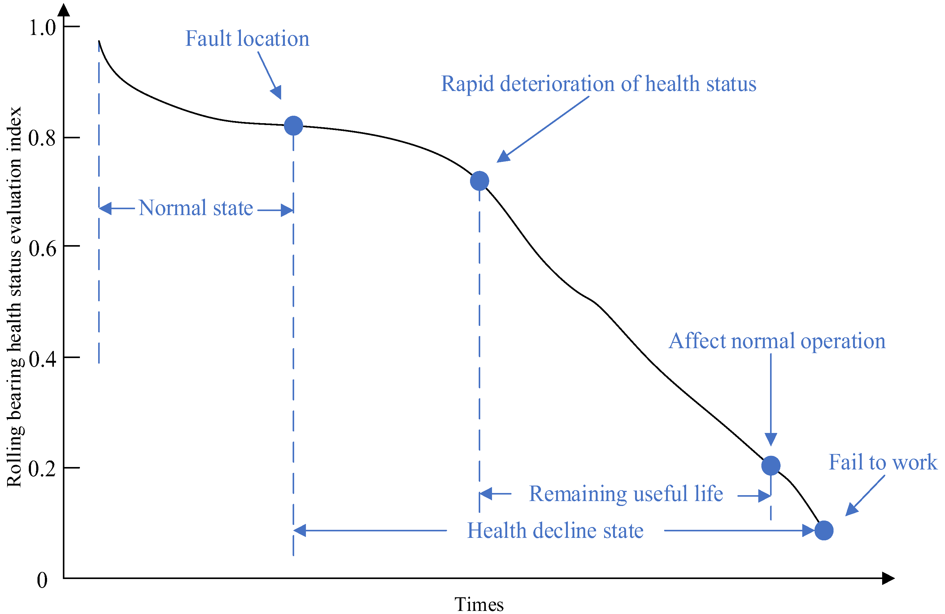
2.4. Health Status Assessment of Rolling Bearings

The health state of the whole life cycle of bearings is mainly divided into four types: normal state, early fault state, moderate fault state, and severe fault state. As shown in Figure 1.

When the bearing works for a long time from the normal state until the failure, its vibration signal will show a corresponding change trend, and finding the characteristics that can best represent the change trend of the bearing state is the most critical step. The root mean square (RMS) in the time domain characteristics will fluctuate significantly with the change of the bearing state during its life cycle. Therefore, RMS of bearing vibration signal is selected as the initial health status evaluation index in this paper.

Although RMS can be used to classify the health status of bearing samples, it has some defects such as inaccurate and delayed sample classification. In order to achieve accurate division, this paper uses the widely used cosine distance (CD) to calculate the similarity between different RMS. The specific steps are as follows:

(1)

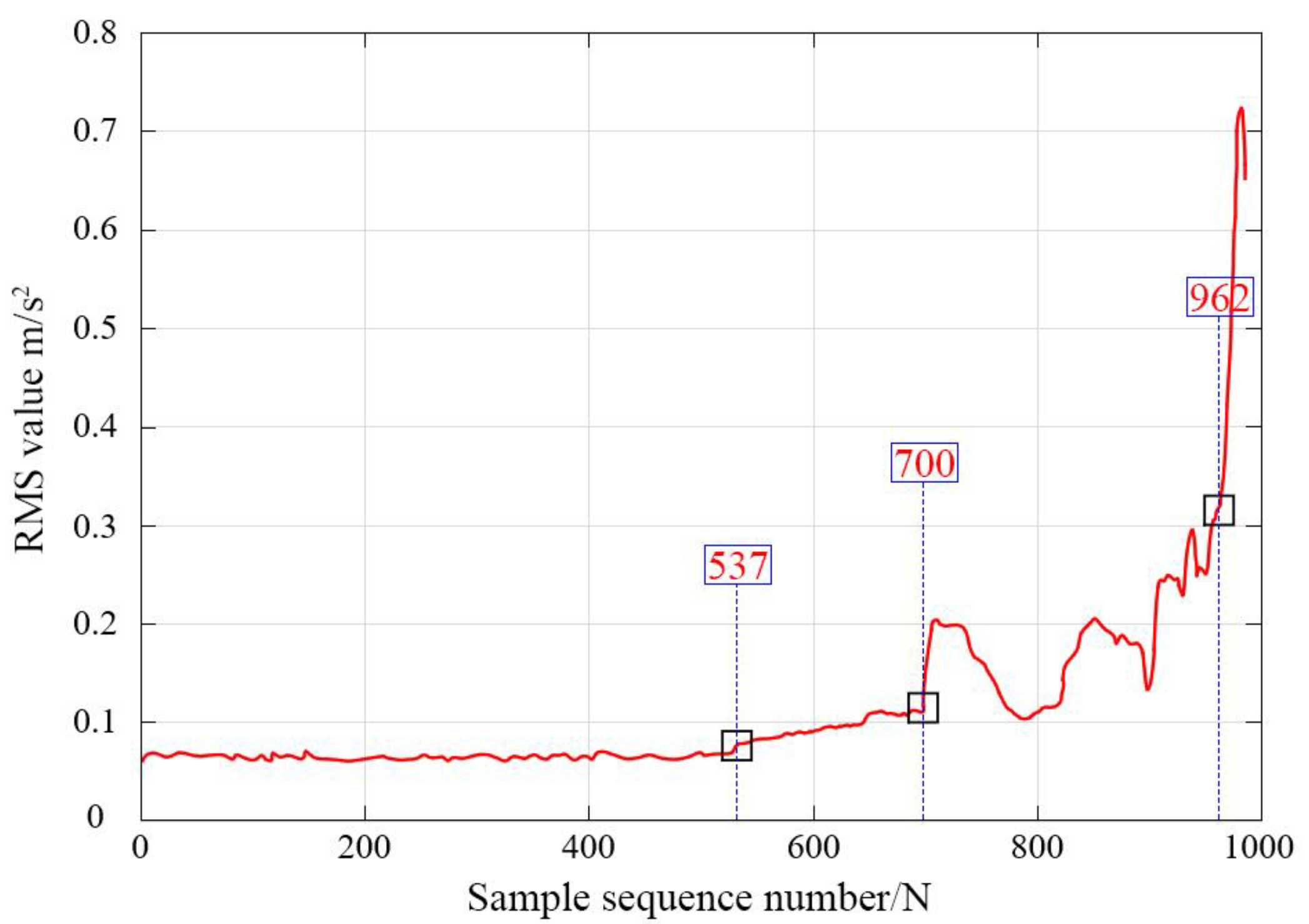
Calculate the RMS X_rms of the bearing vibration signal data, and carry out five-point smoothing processing to eliminate the burr effect caused by noise to determine the change point of the influence state, and draw the RMS change curve of the whole life cycle. The formula is as follows:

$$X_{rms}=\sqrt{\frac{1}{N}{\displaystyle \sum _{i=1}^N{x}_i^2}}$$

(8)

where x_i is a vibration signal sampling value, N is the number of vibration signal sampling.

(2)

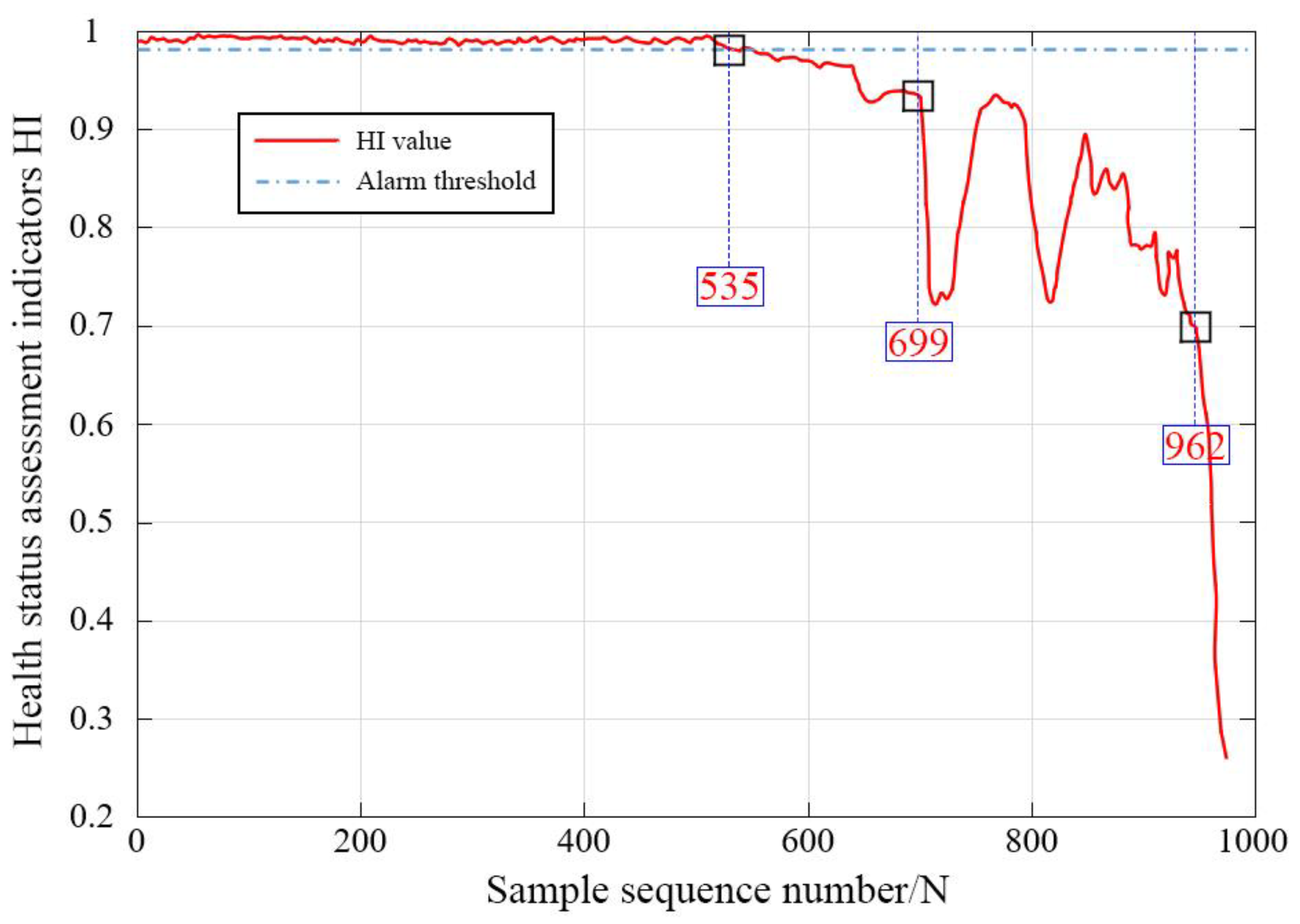
The average of the RMS of the first 6 sample vibration signals after calculation is taken as the normal reference feature vector, and the CD between the feature vectors is calculated. Among them, the similarity between the feature vector to be measured and the normal reference feature vector can be judged by the cosine value of the Angle between them. The closer the cosine value is to 1, the smaller the included angle and the better the health state. Conversely, the smaller the cosine value, the closer the included Angle is to 90°, the worse the health state is. This feature is taken as the final health Index (HI), and plot a smooth curve of changes in health status. The formula is as follows:

$$CD=\frac{{\displaystyle \sum _{i=1}^N{x}_i{y}_i}}{\sqrt{{\displaystyle \sum _{i=1}^N{x}_i^2}}\sqrt{{\displaystyle \sum _{i=1}^N{y}_i^2}}}$$

(9)

(3)

The fault alarm threshold is set using the 3σ rule, and the HI is in line with the normal distribution, with the mean value set as $\bar{x}$ and variance set as σ². The probability that the distribution of HI for the normal state is within the interval ($\bar{x}$ − 3σ, $\bar{x}$ + 3σ) is 99.73%. The mean value and variance are calculated as follows:

$$\overline{x}=\frac{{\displaystyle \sum _{i=1}^n{x}_i}}{n}$$

(10)

$${\sigma }^2=\frac{{\displaystyle \sum _{i=1}^n{\left(x_i-\overline{x}\right)}^2}}{n}$$

(11)

where n is number of samples in normal working state, x_i is the current normal sample HI.

(4)

The HI set in this paper shows a decreasing trend, so it is only necessary to calculate the lower limit $\bar{x}$ + 3σ as the threshold value. When a certain HI value is less than the threshold, it proves that the rolling bearing will deviate from the normal state and enter the early fault state.

3. Bearing Health Management Model Based on SSA-SVM

3.1. Rolling Bearing Fault Diagnosis Model

The signal processing and feature extraction models were constructed using the adaptive parameter VMD-KPCA method, and the detailed process of SVM optimization with SSA algorithm was developed. Therefore, the established fault diagnosis model is shown in Figure 2.

The specific steps are as follow.

(1)

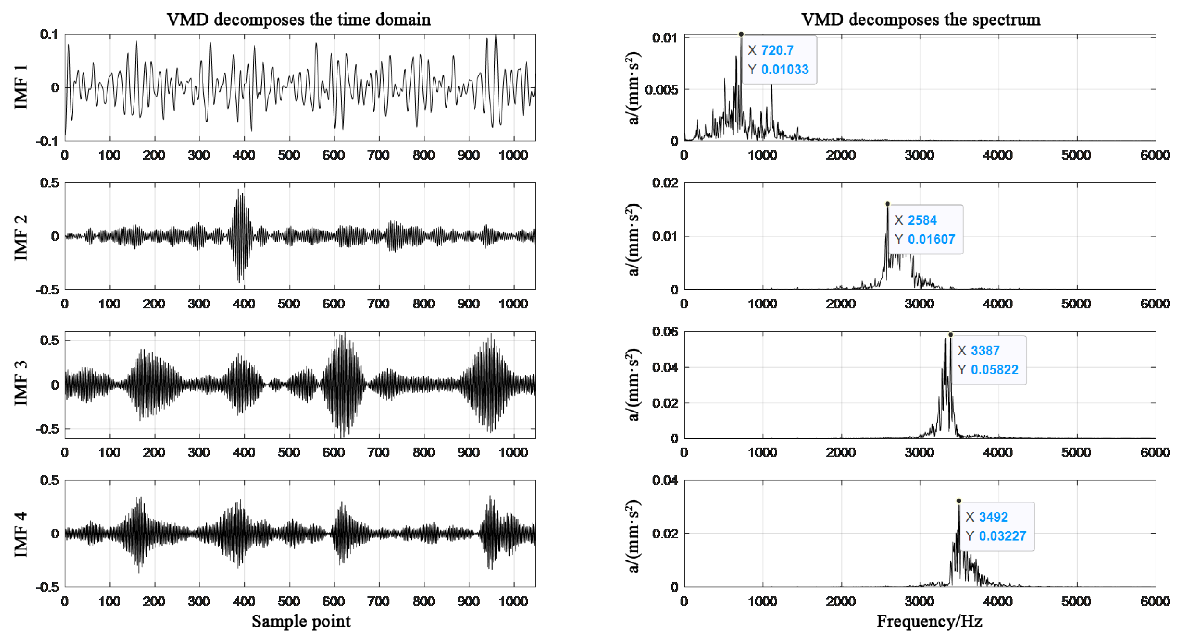
The SSA algorithm is used to optimize the decomposition layer k and penalty factor α in VMD, and the vibration signal is decomposed into multiple intrinsic mode functions (IMFs) to calculate multi-domain features.

(2)

Multivariate characteristics of bearing faults are extracted by KPCA, achieve dimensionality reduction of fault characteristics.

(3)

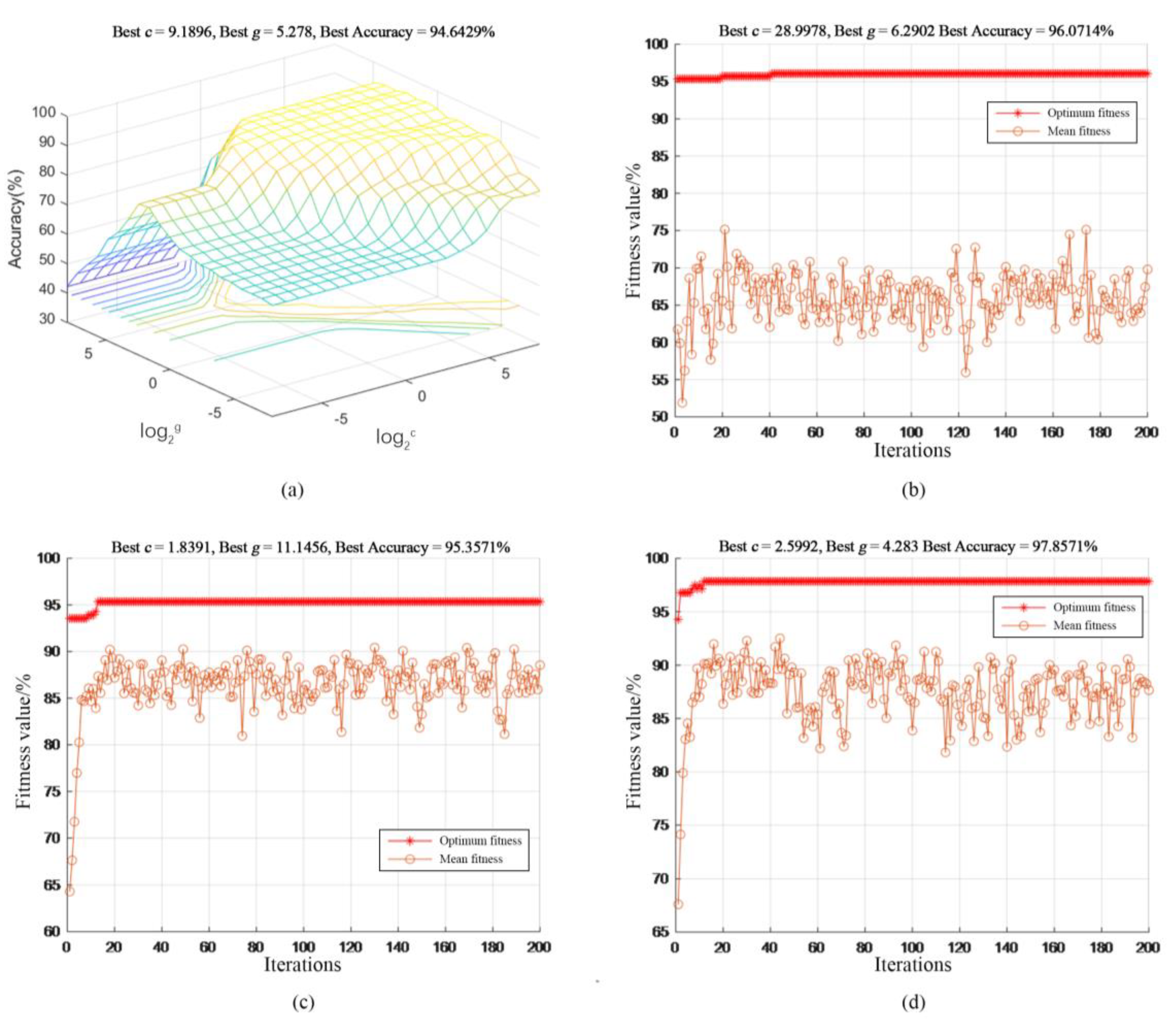
SSA was used to optimize the kernel parameter g and penalty factor c of SVM.

(4)

The extracted fault features are set with type labels in the classifier, and the fault samples are classified by voting method. The diagnosis process is divided into training stage and test stage, and the ratio of training set and test set is 7:3, which is input into the optimized SVM for training.

(5)

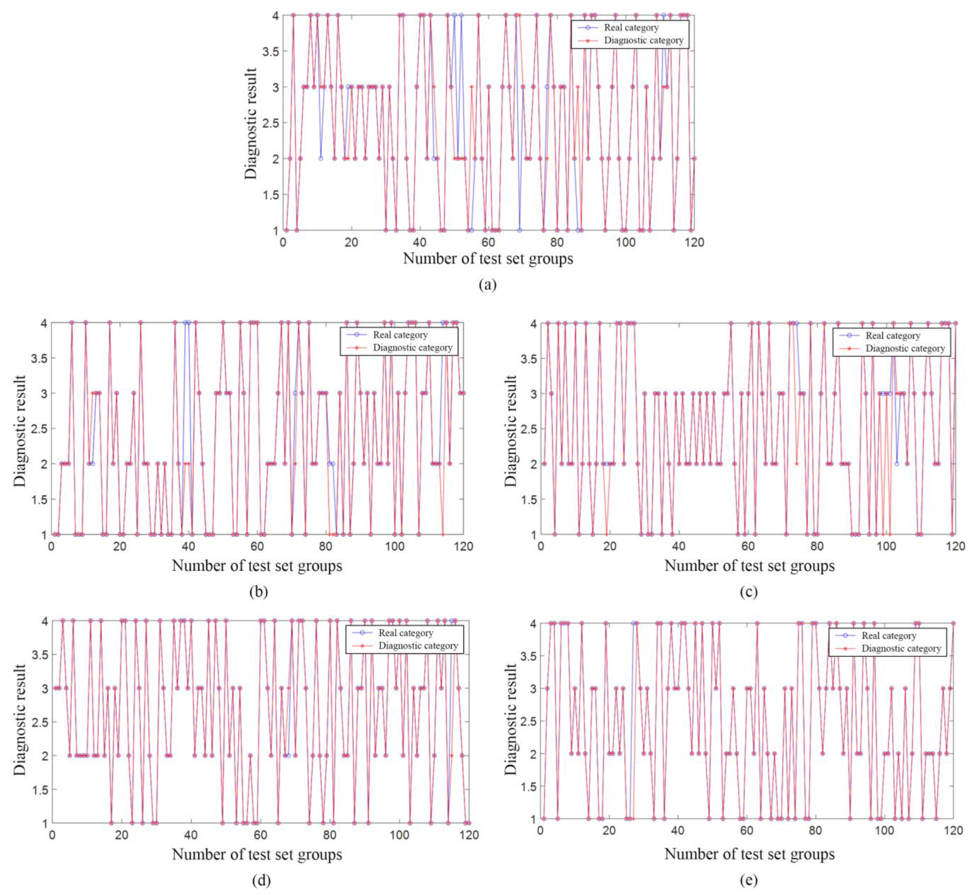
The trained SVM was used to classify and judge different bearing fault samples.

3.2. Rolling Bearing Health Status Evaluation Model

After the construction of the bearing fault diagnosis model, the health status evaluation index and fault alarm threshold are integrated to complete the construction of the rolling bearing health status evaluation model and realize the rolling bearing health management. The model diagram is shown in Figure 3.

The specific steps are as follow.

(1)

Calculate the RMS X_rms of the bearing vibration signal data during the whole life cycle, and perform five-point smoothing processing to eliminate the judgment of the change point of the influence state caused by the burr effect caused by noise, and draw the RMS change curve of the whole life cycle.

(2)

Calculate the cosine distance CD and similarity between feature vectors, construct the health status evaluation index, draw smooth RMS change curve and health status change curve of the whole life cycle, and finally calculate the fault alarm threshold to achieve accurate division of the health status of bearing samples.

(3)

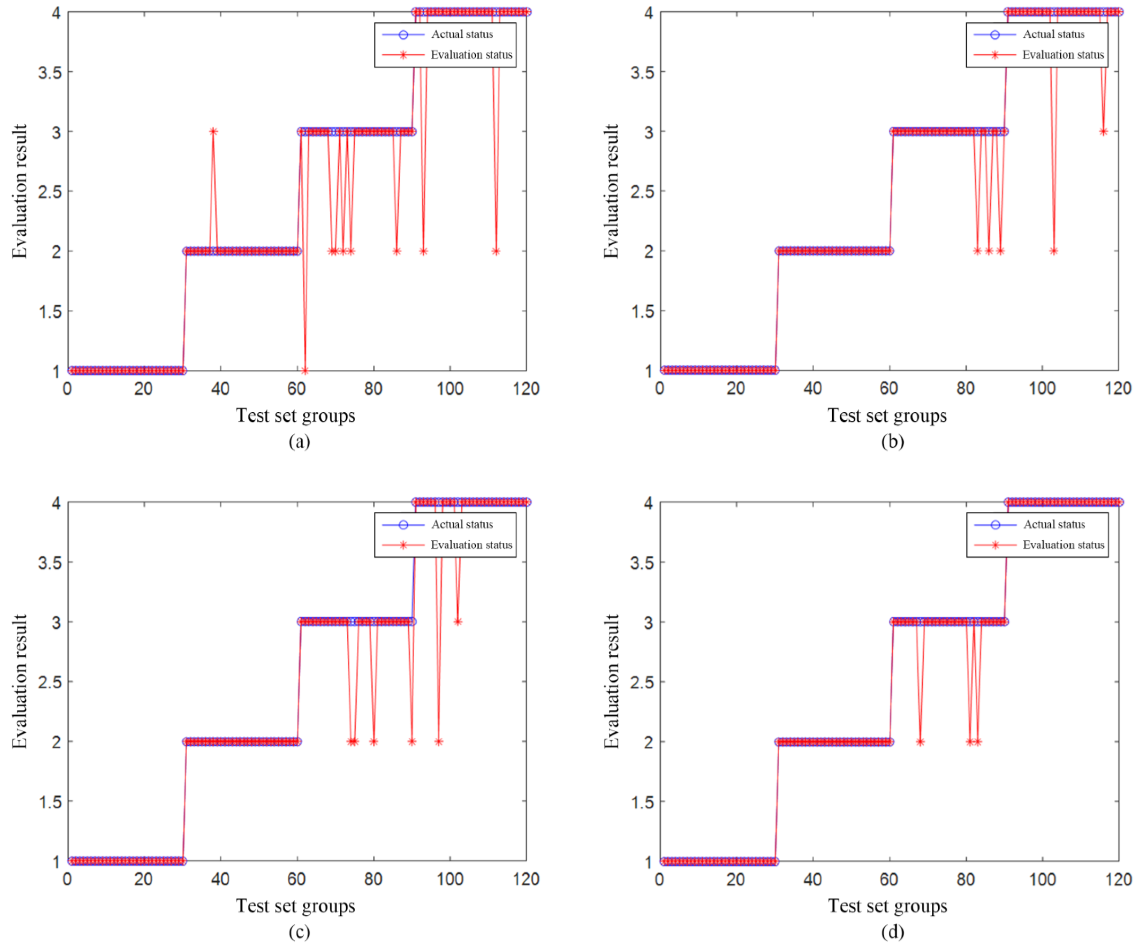
SVM model was constructed using the construction method mentioned above, and four classification labels including normal state, early fault state, moderate fault state and severe fault state were set. The rest process was the same as that of rolling bearing fault diagnosis model construction steps (4).

(4)

Input the training set data into the SVM, and the fitness function is the same as that in the fault diagnosis model. The SSA algorithm is used to obtain the optimal value of the kernel function parameter g and penalty factor c in the SVM to form the SVM optimized by SSA.

(5)

Input the test set samples into the trained SSA-SVM to realize the evaluation of different health states of rolling bearings.

4. Experimental Verification

4.1. Decomposition Processing of Vibration Signal

Test data were obtained from Case Western Reserve University bearing Data center dataset [34] to verify the possibility and superiority of the method described in this paper. The bearing type is 6250-2RS JEM SKF, the motor speed is 1772 r/min, the damage type is single point damage in EDM, and the fault size is 0.007 inch (1 inch = 2.54 cm). At the sampling frequency of using an acceleration sensor is 12 kHz, the original vibration data of the normal state of the bearing at the drive end and the failure of the inner ring, the outer ring and the rolling element were collected. In order to achieve the universal applicability of the model, a total of 400 groups of samples in 4 states were randomly selected. Each group of samples had 1000 sampling points, and the ratio of training set to test set was 7:3.

SSA is used to optimize the decomposition level k and penalty factor α in VMD, where the value range of k and α is [2, 10], [200, 4000], the population size is set to 30, the maximum iteration number is set to 40, and the optimal value of vibration signal samples is tested for 5 times. VMD initialization parameters, the convex function optimization parameter τ is 0, the first center frequency update parameter DC is 0, the center frequency initialization parameter init is 1, and the precision parameter ε is 10⁻⁷. The decomposition results of adaptive VMD decomposition diagram in four running states are shown in Figure 4, Figure 5, Figure 6 and Figure 7. The y-axis of the VMD decomposition diagram is the amplitude of the vibration signal.

Genetic Algorithm (GA) is used to search for the optimal solution by simulating evolutionary selection, hybridization, variation, etc., has a good effect on dealing with complex combination multi-objective problems. Particle Swarm Optimization (PSO) is used to achieve global optimization by simulating the behavior of birds and other groups, and constantly adjusting the speed and direction by changing the learning factor and inertia factor. In order to verify the advantages of SSA algorithm, two classical algorithms, GA and PSO, were used to optimize VMD parameters, and the parameter Settings were the same as those of SSA algorithm. Taking the fault data of rolling bearing outer ring as an example, the vibration signal was decomposed to reduce its background noise. The decomposition results are shown in Figure 8 and Figure 9.

From Figure 4, Figure 5, Figure 6 and Figure 7, it can be seen that in the spectrum diagram of IMF1-IMF4 of the outer ring fault, the center frequency of VMD optimized by SSA does not show mode aliasing phenomenon, and similar results are also found in the other three types of state data. It is proved that the VMD optimized by SSA can effectively decompose the main frequency signals representing fault characteristics from the original bearing signals.

The modal aliasing phenomenon appears in the VMD spectral graph optimized by GA and PSO, which proves that the optimization effect is weaker than SSA algorithm. Among them, the optimal decomposition layers and penalty factor of each state of rolling bearings obtained by SSA optimization of VMD are shown in

Table 1. Parameter results after SSA optimization.

Fault Type	Decomposition Layer k	Penalty Factor α
Normal state	4	2489
Inner ring fault	4	1364
Rolling element fault	4	557
Outer ring fault	4	1439

.

In order to more intuitively reflect the excellent performance of the SSA algorithm, the fitness curves of the three algorithms using the outer ring fault data to optimize VMD parameters were compared, as shown in Figure 10. As can be seen from the figure, SSA-VMD, PSO-VMD and GA-VMD converge in the 6th, 25th, and 36th generations, respectively, and SSA-VMD converges faster. Although all tend to the fitness value of 2.463 in the end, SSA-VMD has the smallest fitness value, which is 2.4633, but also reflects the advantages of its high convergence accuracy.

The time consumed by the three algorithms to optimize VMD parameters and generate vibration signal decomposition is shown in

Table 2. Calculation time of each algorithm.

Algorithm Name	Calculation Time/s
PSO-VMD	639
GA-VMD	658
SSA-VMD	582

. Among them, the average consumption time of PSO-VMD and GA-VMD is similar, while the average consumption time of SSA-VMD is slightly shorter than these two algorithms.

4.2. Feature Extraction and Dimension Reduction Based on KPCA

Considering the advantages of multi-domain parameters on the sensitivity and stability of vibration signals, 16 time domain features and 13 frequency domain features of vibration signals are selected to calculate the IMF component of vibration signals of each fault category after VMD decomposition. At the same time, energy entropy reflects the uniformity of energy distribution and can reflect the complexity of frequencies contained in each IMF component. Therefore, energy entropy of each IMF component is calculated to construct multi-domain high-dimensional fault feature set. The feature formula to be calculated is shown in

Table 3. Multi-domain feature index.

Feature	Calculation Expression	Feature	Calculation Expression	Feature	Calculation Expression
Variance	${\sigma }_x^2=\frac{1}{N-1}{{\displaystyle \sum _{i=1}^N\left(x_i-\overline{X}\right)}}^2$	Maximum value	$X_{\max }=\max \left\{\left|x_i\right|\right\}$	Minimum value	$X_{\min }=\min \left\{x_i\right\}$
Mean value	$\overline{X}=\frac{1}{N}{\displaystyle \sum _{i=1}^N{x}_i}$	Absolute mean	$\left|\overline{X}\right|=\frac{1}{N}{\displaystyle \sum _{i=1}^N\left|x_i\right|}$	Skewness	$\alpha =\frac{1}{N}{\displaystyle \sum _{i=1}^N{x}_i^3}$
Kurtosis	$\beta =\frac{1}{N}{\displaystyle \sum _{i=1}^N{x}_i^4}$	RMS value	$X_{rms}=\sqrt{\frac{1}{N}{\displaystyle \sum _{i=1}^N{x}_i^2}}$	Root amplitude	$X_r={\left[\frac{1}{N}{\displaystyle \sum _{i=1}^N\sqrt{\left|x_i\right|}}\right]}^2$
Peak to peak value	$X_{p-p}=\max \left(x_i\right)-\min \left(x_i\right)$	Peak factor	$C_f=\frac{X_{\max }}{X_{rms}}$	Pulse factor	$I_f=\frac{X_{\max }}{\left|\overline{X}\right|}$
Kurtosis factor	$K_v=\frac{\beta }{X_{rms}^4}$	Waveform factor	$S_f=\frac{X_{rms}}{\left|\overline{X}\right|}$	Margin factor	$C{L}_f=\frac{X_{\max }}{X_r}$
Skewness factor	$P=\frac{\alpha }{X_{rms}^3}$	P1	$P_1=\frac{{\displaystyle \sum _{k=1}^{K}s\left(k\right)}}{K}$	P2	$P_2=\frac{{\displaystyle \sum _{k=1}^K{\left(s\left(k\right)-P_1\right)}^2}}{K-1}$
P3	$P_3=\frac{{\displaystyle \sum _{k=1}^K{\left(s\left(k\right)-P_1\right)}^3}}{K{\left(\sqrt{P_2}\right)}^3}$	P4	$P_4=\frac{{\displaystyle \sum _{k=1}^K{\left(s\left(k\right)-P_1\right)}^4}}{K{P}_2^2}$	P5	$P_5=\frac{{\displaystyle \sum _{k=1}^K{f}_{k}s\left(k\right)}}{{\displaystyle \sum _{k=1}^{K}s\left(k\right)}}$
P6	$P_6=\sqrt{\frac{{\displaystyle \sum _{k=1}^K{\left(f_k-P_5\right)}^{2}s\left(k\right)}}{K}}$	P7	$P_7=\sqrt{\frac{{\displaystyle \sum _{k=1}^K{f}_k^{2}s\left(k\right)}}{{\displaystyle \sum _{k=1}^{K}s\left(k\right)}}}$	P8	$P_8=\sqrt{\frac{{\displaystyle \sum _{k=1}^K{f}_k^{4}s\left(k\right)}}{{\displaystyle \sum _{k=1}^K{f}_k^{2}s\left(k\right)}}}$
P9	$P_9=\frac{{\displaystyle \sum _{k=1}^K{f}_k^{2}s\left(k\right)}}{\sqrt{{\displaystyle \sum _{k=1}^{K}s\left(k\right){\displaystyle \sum _{k=1}^K{f}_k^{4}s\left(k\right)}}}}$	P10	$P_{10}=\frac{P_6}{P_5}$	P11	$P_{11}=\frac{{\displaystyle \sum _{k=1}^K{\left(f_k-P_5\right)}^{3}s\left(k\right)}}{K{P}_6^3}$
P12	$P_{12}=\frac{{\displaystyle \sum _{k=1}^K{\left(f_k-P_5\right)}^{4}s\left(k\right)}}{K{P}_6^4}$	P13	$P_{13}=\frac{{\displaystyle \sum _{k=1}^K{\left(f_k-P_5\right)}^{\frac{1}{2}}s\left(k\right)}}{K{P}_6}$	Energy entropy of each IMF	$\left\{\begin{array}{l}p\left(i\right)=\frac{E\left(c_i\right)}{{\displaystyle \sum _{i=1}^{K}E\left(c_i\right)}}\\ E_q=-{\displaystyle \sum _{i=1}^{K}p\left(i\right)}{\log }_{2}p\left(i\right)\end{array}\right.$

.

Taking the outer ring fault signal as an example, the SSA-VMD method was used to calculate the above multi-domain fault feature indicators by decomposed IMF components. Finally, KPCA algorithm [35,36] was used to calculate the principal component contribution rate of multi-domain features, and screened out the fused core principal component fault features. In the literature, the KPCA screening fault feature threshold CPV ≥ 85% has achieved good results. Therefore, this paper also sets the threshold CPV ≥ 85% to determine s most important main features and constitute the fault feature vector after dimensionality reduction fusion. The principal component contribution rate of KPCA fault characteristics is shown in Figure 11.

Although the cumulative contribution rate of component in Figure 11 is close to 100%, it does not reach 100% in practice, only the top 10 fusion features are shown, and there are still fault features with a small contribution rate. It can be seen from the figure that the cumulative contribution rate of the first four principal component fault feature components is 88.02%, which exceeds the cumulative contribution rate of 85% specified above, and can represent the vast majority of fault characteristics. The multi-domain fault feature can be reduced from 30 to 4 dimensions by sacrificing the component with very small contribution rate, thus achieving the effect of improving the calculation speed.

x_i is the sequence of vibration signal in the time domain, N is the total number of sampling points, s(k) is the amplitude of the k spectrum of bearing vibration signal x_i, K is the number of total spectral lines, f_k is the frequency value of the k spectral line, P₁ is the energy value of bearing vibration signal in the frequency domain. P₂–P₄, P₆, P₁₀–P₁₃ are the dispersion or aggregation levels of the spectrum. In the IMF component energy entropy E_q, c_i is the IMF signal component obtained by decomposition, and p(i) is the energy of all of the obtained IMF signal components normalized. The energy entropy is calculated as follows:

$$E\left(c_i\right)={\displaystyle \sum _{j=1}^N{c}_i{\left(j\right)}^2}$$

(12)

where N is the total number of decomposed signals.

4.3. Identifying Fault Types

In order to prove that the SSA-SVM fault diagnosis model has a higher diagnosis rate, the four types of rolling bearing vibration signals decomposed by SSA-VMD above are input into the unoptimized SVM and PSO-SVM respectively after dimensionality reduction by KPCA. In the GA-SVM and SSA-SVM fault diagnosis models, in order to make the comparison effect more accurate, the population number of the three algorithms is 30, and the maximum number of iterations is 200. In the K-fold cross-validation method, K = 5, 400 data sets are randomly selected, of which 280 are used as training sets and 120 are used as test sets. The fitness curves of the three algorithms for SVM parameter optimization are shown in Figure 12.

As can be seen from the figure, the best fitness, that is, the diagnostic accuracy rate of GA-SVM, PSO-SVM and unoptimized SVM stabilized at 95.351%, 96.0174%, and 94.649% respectively, while the fitness of SSA-SVM fault diagnosis model reached 97.851%. Compared with the other three models, it has higher diagnostic recognition degree.

The penalty factor c and the optimal value of kernel function parameter g solved by the above model are input into the above four fault diagnosis models whose data is the test set sample, and the diagnosis accuracy of the test set is compared. In order to verify the advantages of KPCA algorithm in both diagnostic accuracy and running time, the SSA-SVM fault diagnosis model without KPCA dimension reduction was added, and the diagnostic results were shown in Figure 13. Among them, the diagnostic results 1, 2, 3 and 4 correspond to the normal state of the rolling bearing, the inner ring fault, the outer ring fault and the rolling element fault respectively. The SVM parameter values, diagnostic accuracy and running time pairs of the five diagnostic models are shown in

Table 4. Comparison of simulation results of various fault diagnosis models.

Fault Diagnosis Model	Penalty Factor c	Kernel Function Parameter g	Diagnostic Accuracy/%	Calculation Time/s
GA-SVM	1.8391	11.1456	94.1667	42.879
PSO-SVM	28.9978	6.2902	95.8333	57.985
Unoptimized SVM	9.1896	5.278	91.6667	3.687
SSA-SVM	2.5992	4.283	98.3333	41.438
SSA-SVM without KPCA	1.6857	7.4074	99.1667	57.208

.

As can be seen from Table 4, although the unoptimized SVM has the fastest running speed, its diagnostic accuracy is also the lowest at 91.667%. Although the running speed of SSA-SVM is close to that of GA-SVM, the diagnostic accuracy of SSA-SVM is the highest among the four fault diagnosis models using KPCA dimensionality reduction, reaching 98.333%, which shows that SSA algorithm has achieved excellent results in SVM optimization compared with other classical algorithms. At the same time, although the diagnostic accuracy of SSA-SVM is 0.8334% lower than that of SSA-SVM without KPCA dimensionality reduction, the running time is saved by 27.561%, which proves that the use of KPCA algorithm will sacrifice a small amount of diagnostic accuracy, but will greatly improve the running speed. It is especially suitable for high-dimensional data types such as rolling bearing fault characteristics.

4.4. Test and Verification of Health Status Assessment Model

4.4.1. Assessment and Division of Health Status

The whole life cycle data of rolling bearings from the University of Cincinnati System Center [37] were used as test data to verify the possibility and superiority of the method described in this paper. Bearing type is Rexnord ZA-2115, motor speed is 2000 r/min, sampling frequency is 20 kHz. Test experiments of 4 rolling bearings were carried out in the data set each time. When one of the bearings was damaged, the experiment was immediately stopped. Therefore, the data of each experiment were vibration signal data of the whole life process, and a total of three sets of data were generated. The experimental results are shown in

Table 5. Details of test results.

Data Set Groups	Sample Length	Damaged Bearing	Damaged Location
Data set 1	2156	Bearing 3	Inner ring fault
		Bearing 4	Rolling element fault
Data set 2	984	Bearing 1	Outer ring fault
Data set 3	6324	Bearing 3	Outer ring fault

.

Since the number of samples in data set 1 and data set 3 is too large, the calculation and analysis time will be greatly increased and the accuracy will be reduced. Therefore, this paper selects 984 sets of experimental data of bearing 1 in data set 2 from normal operation to failure due to outer ring damage for analysis of degenerate samples.

In order to verify that the RMS value selected in this paper can effectively divide the characteristics of rolling bearing sample data from normal to failure, the RMS value of 984 groups of test data is calculated and drawn into a curve, as shown in Figure 14.

It can be seen from Figure 14 that the RMS value has been in a relatively stable state before the 537th sample, indicating that the rolling bearing is in normal operation at this stage, and then the value begins to rise slowly, which proves that the bearing health condition begins to decline and early failure occurs (until the value of the 700th sample starts to increase suddenly). And there is a significant increase and decrease fluctuation phenomenon, which proves that the fault of the bearing begins to deteriorate and enters the intermediate fault stage. This situation continues until the 962 sample, and its value begins to increase sharply, which proves that the health state of the bearing is seriously reduced and tends to fail. This stage is a severe fault state.

According to the method constructed above, the RMS value is transformed into the health status evaluation indicator HI, and the mean and variance of the first 200 samples are calculated to obtain the fault alarm threshold. Finally, the change curve of HI value is drawn, as shown in Figure 15.

As can be seen from Figure 15, the HI value has been relatively stable for a long period of time in the early stage, which proves that the bearing is in a normal state during this period. Starting from the 535th sample, the HI value begins to be lower than the alarm threshold, which proves that the bearing is about to enter an early failure state, which is 2 samples earlier than the RMS value change method, that is, 20 min earlier. After that, the HI value began to decline slowly, until the 699th sample, the HI value showed a significant decline, and then there were obvious fluctuations, indicating that the bearing failure repeatedly deepened and wore out. At this stage, the bearing was in a moderate fault state, which was 1 sample earlier than the RMS value change method, that is, 10 min earlier. The detection point of the severe fault state is the same as that of the RMS value change method. In summary, compared with the RMS value change method, the HI value change method can detect the change of bearing health status in advance, and it is feasible.

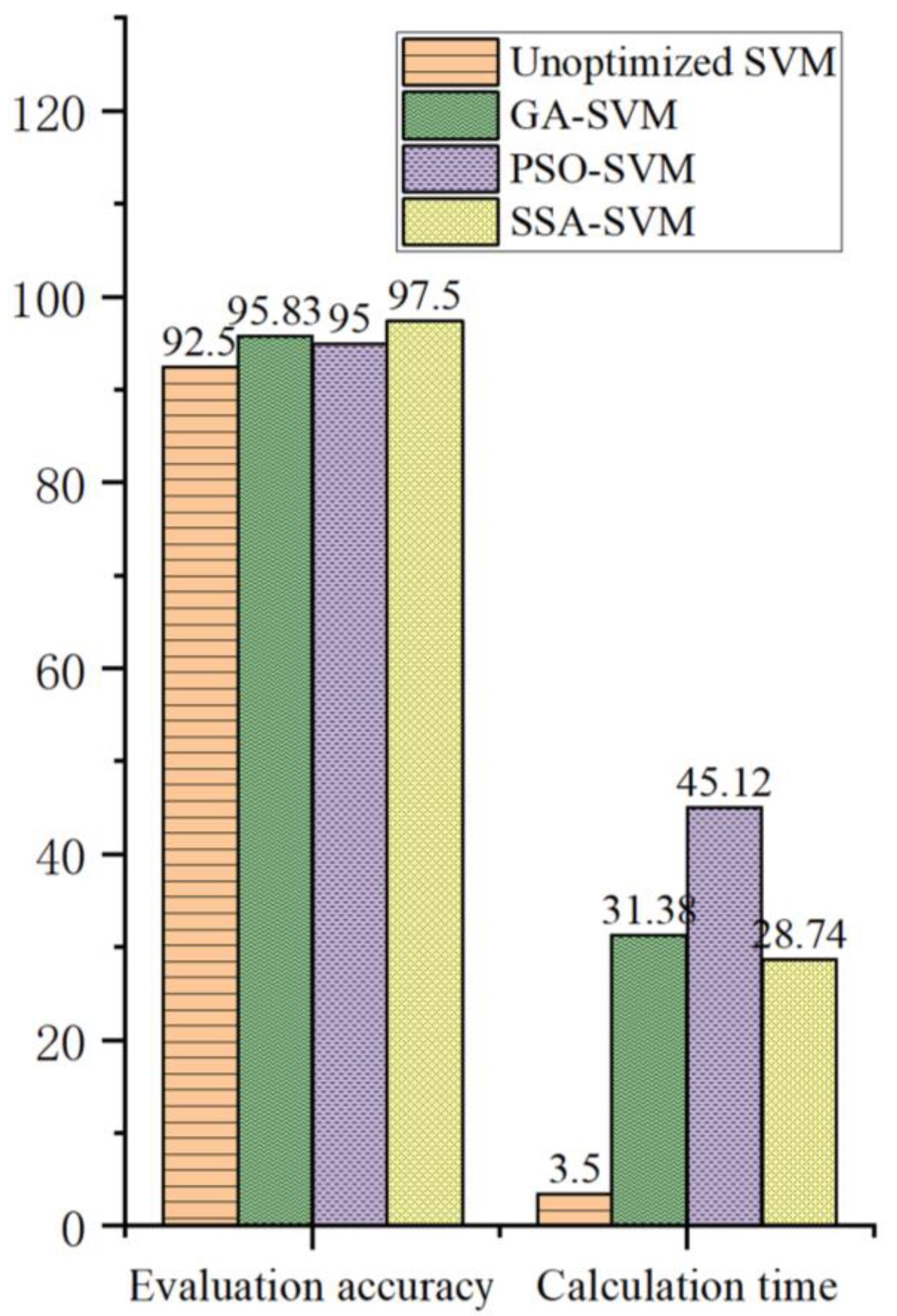
4.4.2. Comparison of Health Status Evaluation Results

The experiments of each algorithm on the optimization process of SVM parameters are consistent with the previous ones, so this paper will not go into details here. The optimal values of kernel function parameter g and penalty factor c optimized by each algorithm were input into the health state evaluation model whose sample was the characteristic data of the test set. The evaluation models were compared in terms of evaluation accuracy and calculation time to verify the advantages of the methods used in this paper. The evaluation results of each model were shown in Figure 16.

From Figure 16, it can be seen that the evaluation error rate of the unoptimized SVM is higher, followed by the SVM optimized by GA and PSO, and the evaluation accuracy of the SSA-SVM method constructed in this paper is the highest. The detailed evaluation of each model is summarized with a bar chart, and the evaluation and results are shown in Figure 17.

As can be seen from Figure 17, although the calculation time of unoptimized SVM 3.498 s is the lowest among the four models, the total number of evaluation errors is the highest. If the sample size continues to increase, a larger error number gap will be formed with other models. The accuracy of the SSA-SVM evaluation model of 97.5% and the computation time of 28.742 s are the best among the three optimized SVM models, which proves the effectiveness of the SSA algorithm in optimizing the kernel function parameter g and penalty factor c in SVM, and also reflects the superiority of the SSA-SVM evaluation model constructed in this paper compared with the other three models. It is suitable for evaluating the health status of rolling bearings during the whole life cycle.

5. Conclusions

In order to improve the accuracy of health monitoring, fault feature extraction and diagnosis of rolling bearings, this paper starts with the signal processing method of VMD-KPCA, the division of degenerate samples based on cosine similarity and sample classification based on SVM, and analyzes the following two aspects of health management of rolling bearings: fault diagnosis and health status assessment, which are studied and verified by an example.

In view of the impact of improper parameter values on the decomposition effect of vibration signals in VMD, the SSA algorithm is used to optimize the number of decomposition layers k and penalty factor α in VMD by using the minimum envelope entropy as the fitness function, and thus an adaptive VMD algorithm is formed according to the difference of vibration signals. Compared with PSO-VMD and GA-VMD, SSA-VMD can effectively suppress the problem of mode aliasing, and the test calculation time is 582 s, which is significantly shortened compared with 639 s and 658 s of PSO-VMD and GA-VMD.

In view of the defect that a single fault feature is easy to cause low fault diagnosis accuracy, this paper uses time domain, frequency domain, and energy entropy to build a multi-domain fault feature set, but high-dimensional fault features will cause a large increase in computation. Therefore, this paper uses KPCA to calculate the principal component contribution rate of multi-domain fault features, eliminates the redundant features, and realizes the dimensionality fusion of fault features.

In order to discover the status changes during the life cycle of rolling bearings in a timely manner, the root-mean-square value of vibration signals is used as the initial health status evaluation index, and then the root-mean-square value is calculated by cosine similarity, which is used as the final health status evaluation index HI, and the 3σ rule is used to integrate the fault alarm threshold. Thus, the fault warning of rolling bearing and the division of sample data are realized.

In view of the difficulty of parameter selection in SVM and the low classification accuracy, this paper uses SSA algorithm to optimize the values of kernel function parameter g and penalty factor c in SVM by taking the optimal value of average classification accuracy in the 5-fold cross-validation as fitness function, and carries out example verification through the authoritative data center data set. The results were compared with the unoptimized SVM, GA-SVM and PSO-SVM models in terms of fault diagnosis accuracy, health status assessment accuracy and calculation time. The results showed that SSA-SVM was superior to other models. The fault diagnosis accuracy of SSA-SVM is 98.3333%, and the state assessment accuracy is 97.5%, which is slightly lower than that of SSA-SVM without KPCA dimensionality reduction, but the calculation time is shortened from 57.208 s to 41.438 s, which is suitable for high-dimensional data types. The accuracy of state evaluation was higher than that of unoptimized SVM, GA-SVM and PSO-SVM, and the computation time of 28.743 s was higher than that of unoptimized SVM (3.498 s), but its accuracy of 92.5% was too low.

In future studies, we should continue to optimize the model to shorten the running time of the model, improve the accuracy and robustness of the model. In the data set test phase, we can select the data under varying conditions to verify the generalization performance of the model. In addition, we can also improve the overall information integration capability of the model, establish a lighter weight, economic and flexible bearing health management system, and integrate the updated model into the existing model to improve the model capability.

References

1. Ding, X.; He, Q.; Luo, N. A fusion feature and its improvement based on locality preserving projections for rolling element bearing fault classification. J. Sound Vib. 2015, 335, 367–383. [Google Scholar] [CrossRef]
2. Jiang, L.; Sheng, H.; Yang, T.; Tang, H.; Li, X.; Gao, L. A New Strategy for Bearing Health Assessment with a Dynamic Interval Prediction Model. Sensors 2023, 23, 7696. [Google Scholar] [CrossRef]
3. Liu, M.; Fan, H.; Zhang, Y.; Li, Z.; Yang, W. Adaptive multi-scale method for the non-linear dynamic feature extraction of mechanical vibration signals. J. Vib. Shock 2020, 39, 224–232. [Google Scholar] [CrossRef]
4. Qian, M.; Yu, Y.; Guo, L.; Gao, H.; Zhang, R.; Li, S. A new health indicator for rolling bearings based on impulsiveness and periodicity of signals. Meas. Sci. Technol. 2022, 33, 105008. [Google Scholar] [CrossRef]
5. Jinwoo, S.; Seokgoo, K.; Woo, L.S.; Jinhong, M.; Joo-Ho, C. Construction of bearing health indicator under time-varying operating conditions based on Isolation Forest. Eng. Appl. Artif. Intell. 2023, 126, 107058. [Google Scholar] [CrossRef]
6. Wang, X.; Zheng, J.; Ni, Q.; Pan, H.; Zhang, J. Traversal index enhanced-gram (TIEgram): A novel optimal demodulation frequency band selection method for rolling bearing fault diagnosis under non-stationary operating conditions. Mech. Syst. Signal Process. 2022, 172, 109017. [Google Scholar] [CrossRef]
7. Liu, Y.; Kang, J.; Bai, Y.; Guo, C. Research on the health status evaluation method of rolling bearing based on EMD-GA-BP. Qual. Reliab. Eng. Int. 2023, 39, 2069–2080. [Google Scholar] [CrossRef]
8. Aggarwal, A.; Malik, H.; Sharma, R. Feature Extraction using EMD and Classification through Probabilistic Neural Network for Fault Diagnosis of Transmission line. In Proceedings of the IEEE International Conference on Power Electronics, Intelligent Control and Energy Systems, Delhi, India, 4–6 July 2016. [Google Scholar]
9. Qi, X.; Ye, X.; Cai, J.; Zheng, J.; Pan, Z.; Zhang, X. Fault feature extraction method of rolling bearings based on VMD and manifold learning. J. Vib. Shock 2018, 37, 133–140. [Google Scholar] [CrossRef]
10. Dragomiretskiy, K.; Zosso, D. Variational Mode Decomposition. IEEE Trans. Signal Process. 2014, 62, 531–544. [Google Scholar] [CrossRef]
11. Lu, Z.; Wang, Z.; Yan, X.; Liu, D.; Sun, J.; Ma, C. Research Progress in Application of Variational Mode Deomposition Method in Bearing Fault Diagnosis. Lubr. Eng. 2023. in press. Available online: http://kns.cnki.net/kcms/detail/44.1260.TH.20231207.1359.044.html (accessed on 8 December 2023).
12. Wu, Z.; Li, H.; Wang, T. Research on Fault Diagnosis of Rolling Bearing Based on Trend-guided VMD. Mach. Des. Manuf. 2023; in press. [Google Scholar] [CrossRef]
13. Wang, X.; Jiang, B.; Xiao, L.; Ma, L.; Chen, Y. AMO-VMD data processing method for high-speed bearing fault under variable working conditions. Control Theory Appl. 2023, 40, 1–8. [Google Scholar]
14. Wu, Z.; Zhang, Z.; Zheng, L.; Yan, T.; Tang, C. The Denoising Method for Transformer Partial Discharge Based on the Whale VMD Algorithm Combined with Adaptive Filtering and Wavelet Thresholding. Sensors 2023, 23, 8085. [Google Scholar] [CrossRef] [PubMed]
15. Jiang, T.; Li, Y.; Li, S. Multi-fault diagnosis of rolling bearing using two-dimensional feature vector of WP-VMD and PSO-KELM algorithm. Soft Comput. 2022, 27, 8175–8187. [Google Scholar] [CrossRef]
16. Peng, Z.; Bai, H.; Shiina, T.; Deng, J.; Liu, B.; Zhang, X. LED-Lidar Echo Denoising Based on Adaptive PSO-VMD. Information 2022, 13, 558. [Google Scholar] [CrossRef]
17. Ni, Q.; Ji, J.; Feng, K.; Halkon, B. A fault information-guided variational mode decomposition (FIVMD) method for rolling element bearings diagnosis. Mech. Syst. Signal Process. 2022, 164, 108216. [Google Scholar] [CrossRef]
18. Pawel, Z. Influence of bearing raceway surface topography on the level of generated vibration as an example of operational heredity. Indian J. Eng. Mater. Sci. 2020, 27, 356–364. [Google Scholar]
19. Vivek, P.; Huzur, S.; Suraj, P.H. An autonomous method for diagnosing raceway defects and misalignment in a self-aligning rolling-element bearing. Proc. Inst. Mech. Eng. Part K J. Multi-Body Dyn. 2022, 236, 470–487. [Google Scholar] [CrossRef]
20. Huang, J.; Cui, L.; Zhang, J. Novel morphological scale difference filter with application in localization diagnosis of outer raceway defect in rolling bearings. Mech. Mach. Theory 2023, 184, 105288. [Google Scholar] [CrossRef]
21. Chen, R.; Liu, J.; Tang, J.; Han, Q.; Zhang, Y.; Cui, Y. Vibration characteristics analysis of rolling bearing rotor system considering radial clearance and outer raceway defect. Adv. Mech. Eng. 2023, 15, 4. [Google Scholar] [CrossRef]
22. Li, Y.; Zhang, W.; Xiong, Q.; Luo, D.; Mei, G.; Zhang, T. A rolling bearing fault diagnosis strategy based on improved multiscale permutation entropy and least squares SVM. J. Mech. Sci. Technol. 2017, 31, 2711–2722. [Google Scholar] [CrossRef]
23. Zhou, J.; Xiao, M.; Niu, Y.; Ji, G. Rolling Bearing Fault Diagnosis Based on WGWOA-VMD-SVM. Sensors 2022, 22, 6281. [Google Scholar] [CrossRef] [PubMed]
24. Song, X.; Wei, W.; Zhou, J.; Ji, G.; Hussain, G.; Xiao, M.; Geng, G. Bayesian-Optimized Hybrid Kernel SVM for Rolling Bearing Fault Diagnosis. Sensors 2023, 23, 5137. [Google Scholar] [CrossRef] [PubMed]
25. Saeed-Nezamivand, C.; Ahmad, B.; Farid, N. A new intelligent fault diagnosis method for bearing in different speeds based on the FDAF-score algorithm, binary particle swarm optimi- zation, and support vector machine. Soft Comput. 2019, 23, 1–19. [Google Scholar] [CrossRef]
26. Javed, K.; Gouriveau, R.; Zerhouni, N.; Nectoux, P. Enabling Health Monitoring Approach Based on Vibration Data for Accurate Prognostics. IEEE Trans. Ind. Electron. 2015, 62, 647–656. [Google Scholar] [CrossRef]
27. Li, Z.; Fang, H.; Huang, M.; Wei, Y.; Zhang, L. Data-driven bearing fault identification using improved hidden Markov model and self-organizing map. Comput. Ind. Eng. 2018, 116, 37–46. [Google Scholar] [CrossRef]
28. Dong, X.; Cao, Y.; Li, H.; Han, X.; Feng, W. Performance Degradation Evaluation Model of Rolling Bearing Based on CAE-SVDD; Springer Nature: Cham, Switzerland, 2023; pp. 341–353. [Google Scholar] [CrossRef]
29. Liao, A.; Wu, Y.; Ding, Y. Performance degradation evaluation of rail vehicle bearing based on PSO-OEWOA and MKSVDD. J. Railw. Sci. Eng. 2022, 19, 2730–2738. [Google Scholar] [CrossRef]
30. Lei, Y.; Li, N.; Guo, L.; Li, N.; Yan, T.; Lin, J. Machinery health prognostics: A systematic review from data acquisition to RUL prediction. Mech. Syst. Signal Process. 2018, 104, 799–834. [Google Scholar] [CrossRef]
31. Yang, S.; Tang, B.; Wang, W.; Yang, Q.; Hu, C. Physics-informed multi-state temporal frequency network for RUL prediction of rolling bearings. Reliab. Eng. Syst. Saf. 2024, 242, 109716. [Google Scholar] [CrossRef]
32. Mohit, J.; Vijander, S.; Asha, R. A novel nature-inspired algorithm for optimization: Squirrel search algorithm. Swarm Evol. Comput. 2018, 44, 1–28. [Google Scholar] [CrossRef]
33. Xin, X. Support Vector Machine Theory, Algorithm and Implementation. Master’s Thesis, Information Engineering University, Zhengzhou, China, 2005. [Google Scholar]
34. The Case Western Reserve University. Bearing Data Center Seeded Fault Test Data. Available online: https://engineering.case.edu/bearingdatacenter (accessed on 27 December 2021).
35. Jiang, L.L.; Li, P.; Tang, S.W. Parameter Optimization in KPCA for Rotating Machinery Feature Vector Dimensionality Reduction. Adv. Eng. Forum 2011, 1598, 755–760. [Google Scholar] [CrossRef]
36. Chen, P.; Zhao, X.; Zhu, X. Fault diagnosis method of rolling bearing based on VMD-MPE-KPCA feature extraction mixed with MRVM. J. Lanzhou Univ. Technol. 2020, 46, 92–99. [Google Scholar]
37. Bearin Data Set in NASA Ame Prognostic Data Repository. Available online: http://ti.arc.nasa.gov/project/prognostic-data-repository (accessed on 19 March 2022).
Figure 1. Schematic diagram of the change trend of rolling bearing health status.
Processes 12 00433 g001
Figure 2. Rolling bearing fault diagnosis model.
Processes 12 00433 g002
Figure 3. Rolling bearing health status evaluation model.
Processes 12 00433 g003
Figure 4. Adaptive parameters VMD decomposition diagram of normal state.
Processes 12 00433 g004
Figure 5. Adaptive parameters VMD decomposition diagram of inner ring fault.
Processes 12 00433 g005
Figure 6. Adaptive parameters VMD decomposition diagram of rolling element fault.
Processes 12 00433 g006
Figure 7. Adaptive parameters VMD decomposition diagram of outer ring fault.
Processes 12 00433 g007
Figure 8. GA-VMD decomposition diagram of outer ring fault.
Processes 12 00433 g008
Figure 9. PSO-VMD decomposition diagram of outer ring fault.
Processes 12 00433 g009
Figure 10. Failure fitness curve of the outer ring.
Processes 12 00433 g010
Figure 11. KPCA principal component contribution Pareto diagram.
Processes 12 00433 g011
Figure 12. SVM parameter optimization process. (a) Unoptimized SVM parameter selection results. (b) PSO-SVM parameter optimization process. (c) GA-SVM parameter optimization process. (d) SSA-SVM parameter optimization process.
Processes 12 00433 g012
Figure 13. Fault diagnosis results of the diagnostic model. (a) Unoptimized SVM fault diagnosis results. (b) GA-SVM fault diagnosis results. (c) PSO-SVM fault diagnosis results. (d) SSA-SVM fault diagnosis results. (e) SSA-SVM fault diagnosis results without KPCA.
Processes 12 00433 g013
Figure 14. Changes in RMS value of lifetime data.
Processes 12 00433 g014
Figure 15. Changes in HI value of lifetime data.
Processes 12 00433 g015
Figure 16. Health status evaluation model results. (a) Unoptimized SVM health status evaluation results. (b) GA-SVM health status evaluation results. (c) PSO-SVM health status evaluation results. (d) SSA-SVM health status evaluation results.
Processes 12 00433 g016
Figure 17. Comparison of the results of health status evaluation models.
Processes 12 00433 g017