Article

A Fault-Tolerant Soft Sensor Algorithm Based on Long Short-Term Memory Network for Uneven Batch Process

College of Control Science and Engineering, Zhejiang University, Hangzhou 310058, China
*
Author to whom correspondence should be addressed.
Processes 2024, 12(3), 495; https://doi.org/10.3390/pr12030495
Submission received: 29 January 2024 / Revised: 24 February 2024 / Accepted: 25 February 2024 / Published: 28 February 2024
(This article belongs to the Section Process Control and Monitoring)

Abstract

:
Batch processing is a widely utilized technique in the manufacturing of high-value products. Traditional methods for quality assessment in batch processes often lead to productivity and yield losses because of offline measurement of quality variables. The use of soft sensors enhances product quality and increases production efficiency. However, due to the uneven batch data, the variation in processing times presents a significant challenge for building effective soft sensor models. Moreover, sensor failures, exacerbated by the manufacturing environment, complicate the accurate modeling of process variables. Existing soft sensor approaches inadequately address sensor malfunctions, resulting in significant prediction inaccuracies. This study proposes a fault-tolerant soft sensor algorithm that integrates two Long Short-Term Memory (LSTM) networks. The algorithm focuses on modeling process variables and compensating for sensor failures using historical batch quality data. It introduces a novel method for converting quality variables into process rates to align uneven batch data. A case study on simulated penicillin production validates the superiority of the proposed algorithm over conventional methods, showing its capacity for precise endpoint detection and effectiveness in addressing the challenges of batch process quality assurance. This study offers a robust solution to the issues of soft sensor reliability and data variability in industrial manufacturing.

1. Introduction

Batch processing is a quintessential procedure in the industry, extensively employed in diverse fields, including semiconductor manufacturing, biopharmaceutical production, culinary processing, polymerization reactions, metallurgical processing, and others. Due to the end products’ high value, rigorous quality monitoring and precise measurements are essential. In contrast to continuous industrial processes, batch processes exhibit greater complexity in their characteristics and a more pronounced abundance of statistical attributes within their data. Among their features, the most crucial aspect is that in batch processes, product quality variables are often only detectable offline at the end of the production cycle, rendering real-time measurement impossible.
In recent years, data-driven soft sensors have emerged for industrial production. Soft sensors can estimate post-process quality variables using real-time signal data [1]. Essentially, soft sensors serve as regression models for linking hard-to-measure quality variables with easy-to-measure process variables. Soft sensors have gained widespread adoption in various industries due to their ability to significantly reduce time and cost.
The application of soft sensors in industrial processes is also extensive. On the one hand, soft sensors can assist with quality control. It maintains consistent product quality by providing estimates of critical quality variables [2]. This approach minimizes reliance on costly or delayed laboratory analyses, reducing the incidence of non-conforming products and optimizing operational efficiency and product reliability [3]. For example, in the semiconductor field, due to the complexity of the process, sampling tests have to be carried out after each process on a batch-by-batch basis [4]. With soft sensors, the process quality of each wafer can be precisely controlled [5]. On the other hand, soft sensors enable real-time control. Integrating soft sensors with real-time control facilitates optimizing the control strategy and enhances the system’s ability to address process disturbances preemptively [6]. By providing a more detailed process state, including previously unmeasured variables, control systems can identify trends and deviations earlier, enabling proactive adjustments that minimize the impact of disturbances and maintain steady operation [7]. For example, establishing a soft sensor for debutanizer distillation columns can overcome the considerable time delays associated with the corresponding gas chromatograph and provide real-time concentrations of the top and bottom products in the column, facilitating reaction evaluation, monitoring, and control [8].
The prevailing soft sensor methods currently include both linear and nonlinear approaches. Linear methods include partial least square (PLS) [9,10] and multiple linear regression (MLR) [11] and Lasso [12]. Nonlinear methods include support vector regression (SVR) [13] and artificial neural networks (ANNs) [14,15]. However, due to the multitude of variables and complex responses in the process, these methods often struggle to achieve high accuracy.
Industrial processes, which are typically complex and nonlinear, often contain a significant amount of information about quality variables within their process variables. The complexity of this task makes it challenging to extract such information using simply structured machine learning algorithms. Deep learning methods excel at extracting detailed information from time series data, making them widely adopted for modeling soft sensors in recent times. Recurrent neural network (RNN) and long short-term memory (LSTM) networks have been effectively applied to create soft sensor models across various industrial domains, including the chemical industry [16], coal gasification [17], hydrocracking process [18], wastewater treatment [19], as well as semiconductor manufacturing [20]. Additionally, Stacked Autoencoders (SAEs) and their variations have also been commonly employed in creating soft sensors for industrial processes [21,22].
However, data-driven soft sensors heavily rely on process data and are therefore vulnerable to sensor failures [23]. The data used to model these soft sensors are obtained from physical sensors that monitor various process parameters. These sensors are distributed throughout a plant and are exposed to long-term wear and tear, extreme temperatures, pressures, and chemical environments. Such conditions can lead to sensor contamination, degradation, and failure, resulting in both linear and nonlinear measurement errors in process variables. The failure of a single physical sensor has a more pronounced impact on the failure rate of soft sensors compared to its isolated effect. Soft sensors rely on data from multiple physical sensors. Therefore, when even one sensor fails, it can significantly amplify the overall failure rate, leading to deviations in process data. This vulnerability becomes so pronounced that significant discrepancies occur between the estimates of soft sensor and actual values. For instance, deep neural networks (DNNs) demonstrate a significant vulnerability to sensor failures [24]. While DNN-based soft sensors may perform with high accuracy initially, their effectiveness can sharply decline when physical sensors malfunction post-online deployment. This sensitivity to sensor failure severely restricts the practical applicability of DNN-based soft sensors in industrial settings. The challenge lies in developing soft sensor models that are not only accurate under stable conditions but also maintain their precision and reliability in the face of sensor failures. This is a critical requirement for their successful application in real-world industrial processes.
In addition, addressing the issue of uneven batches is crucial when developing soft sensors for batch processes. This challenge arises because the data from different batches may not form a neat three-dimensional matrix. Typically, time-series data are characterized by sequences uniform in time intervals and length, enabling effective processing by many time-dependent algorithms. However, achieving such consistency across batches in real-world production processes is often impractical due to various factors, resulting in significant variations in the data length for each batch. The primary issue with modeling uneven batch data is data alignment. The challenge lies in handling this alignment optimally to ensure the complete extraction of information from the batch data. Practical strategies for data alignment and handling uneven batches are essential to capture the full scope of process variability and enhance the performance and reliability of the soft sensor in real-world applications.
Inspired by the idea of drift sensor compensation utilizing historical quality data [25], this paper proposes a fault-tolerant soft sensor algorithm based on a two-layer LSTM model to address the issue of varying batch data lengths. It achieves this by converting quality metrics into process rate estimations using fixed windows. The main contributions of this paper are as follows:
  • An algorithm based on a two-layer LSTM model is proposed to develop a fault-tolerant soft sensor for modeling long-time nonlinear dependent batch processes. Historical batch data quality measurements are applied to the soft sensor to enhance the robustness of the model in case of sensor failure;
  • The problem of estimating the quality variable of uneven batch processes is transformed into rate estimation within a fixed window, which addresses the issue of uneven batch data. The model’s reliability is verified on normal data and datasets with various failures in simulated penicillin production;
  • An algorithm for endpoint detection is proposed to estimate the quality variable using the soft sensor model, which can accurately determine when to terminate production once the expected yield is reached.

2. Related Work

2.1. Sensor Fault-Tolerant

In industrial production, the frequent occurrence of sensor aging and failures demands a dual focus on soft sensor modeling. While achieving high-quality estimations under normal conditions is essential, it is equally, if not more, vital to maintaining reliable soft sensor accuracy during sensor failures. A sensor failure is characterized by a linear or nonlinear discrepancy between the measured and actual values before the failure. Despite this deviation, the sensor’s measured data continues to provide valuable information about the production process. The challenge lies in effectively utilizing indirect information to compensate for inaccuracies in sensor measurements, thereby developing fault-tolerant soft sensors. This involves implementing complex strategies to identify and rectify errors caused by sensor degradation or failure, guaranteeing that the soft sensor maintains its robustness and reliability even when sensor faults occur.
In industrial production, sensor failures occur frequently. Sensor failures are generally categorized as abrupt offset and slow drift faults (degradation). Generally speaking, the study of sensor fault-tolerant in industrial processes combines fault diagnosis and process control. For example, a data-driven fault-compensated tracking control system is designed for a coupled wastewater treatment process with sensor faults, and an adaptive fault compensation mechanism is constructed [26]. Yang et al. propose a strategy for air conditioning systems to correct mismeasurements using a final correction factor [27]. This model requires a high level of computational accuracy. In addition, the evaluation thresholds and weighting factors depend on manual assignment. A hybrid model-based and data-driven approach is proposed to diagnose current sensor faults in single-phase pulse-width modulated rectifiers [28]. Most of these methods utilize control feedback loops or redundant backups to correct sensor failures.
The growing emphasis on soft sensors in recent years has led to the development of several industrial fault-tolerant soft sensors. These advanced systems are designed to maintain accuracy and reliability despite sensor failures and other anomalies common in industrial environments. A deep subdomain learning adaptation network is proposed to handle both sensor degradation and sensor failure [24]. This approach applies to continuous processes in which the subdomain structure of each sample follows a classification distribution parameterized by the output of the subdomain learner. The effect is not validated for batch processes with significant variation. Aiming to decentralize the dissolved oxygen control process, a data-driven soft sensor is established as a backup for the joint sensor and controller block to overcome the failure of the dissolved oxygen sensor using an adaptive neuro-fuzzy inference system [29]. Nonetheless, the fuzzy modeling knowledge of this approach needs to be acquired through manual synthesis of the process operating state and time-consuming manual interventions to set the design parameters. Three new fault-tolerant soft sensor algorithms are proposed based on measurement space tool subspace design, respectively, which eliminate the effects caused by sensor failures through optimal estimation and orthogonality properties [30]. However, these methods rely on the knowledge of the operation of sensors and actuators in dynamic systems and can only be applied to continuous processes.
In summary, current research on sensor fault-tolerant soft sensors is still limited, with a predominant focus on continuous processes. This focus leaves a notable gap in the context of batch processes, which present unique challenges due to their uneven lengths and variable nature. Therefore, this study aims to explore and develop a sensor fault-tolerant soft sensor algorithm specifically designed for batch processes.

2.2. Uneven Batches

In batch processes, the operation duration may differ from batch to batch due to unavoidable disturbances. Changes in initial conditions and other factors can lead to varying batch lengths [31]. Since general time series methods can only be applied to matrices, and uneven batch data cannot be structured as such, the data must be preprocessed before soft sensor modeling. A straightforward approach to address this challenge is to cut all batch data to match the length of the shortest batch [32]. It is clear that this simple method leads to the loss of valuable information. An alternative strategy involves increasing the length of shorter batch datasets. This is achieved by padding these batches with zero values until they reach the maximum length observed in the batch set [33]. Dynamic Time Warping (DTW) is also an approach that has achieved universal application [34]. In addition, various modifications of DTW have been utilized for aligning uneven batches of data [35,36]. Nevertheless, they run the risk of distorting the relationship between process variables [37]. Another common approach is to resample process variables using methods such as interpolation, which has now gained applications in areas such as fault diagnosis [38]. The RGTW-MOENPE algorithm is introduced to align batch processes, having varied durations while preserving the essential features of critical events [37]. A dynamic multi-stage and multi-mode modeling approach is proposed [39]. For batches, phasing is performed, local dynamic behavior is described, and operating modes are clustered based on global differences.
While attempting to align batch data, current approaches often introduce complexity, overlook the dynamic relationship between variables over time, or distort the correlations among variables. The complexity hinders the development of high-precision soft sensors in industrial processes. An ideal solution should be easy to implement yet sophisticated enough to maintain the temporal dynamics and variable correlations within the batch data. This solution should accommodate varying batch lengths without introducing significant distortions or complexities that could compromise the model’s accuracy and reliability.

2.3. LSTM-Based Soft Sensor

As stated in the abstract, due to the temporal dynamics of data sequences in industrial processes, methods represented by LSTM and their variants have been widely used in soft sensors for industrial processes [40]. A batch-training-based bi-directional LSTM soft sensor modeling method is proposed [41]. The reconstructed segmented training samples using a variational autoencoder are utilized to solve the problem of global LSTM models discarding crucial data information during training. This method reduces noise and improves the accuracy of soft sensors in the grinding and classifying process dataset. However, it is limited to a single operating condition and does not consider the internal properties of the variables. A supervised LSTM network is proposed for learning quality-related hidden dynamics in soft sensor applications, where both quality variables and input variables are used in the basic unit of the network to learn dynamic hidden states that are more relevant and useful for quality prediction [42]. The method enhances the accuracy of variable selection, but it only considers hidden states at a single moment in time, neglecting the relationships between variables and within the process. Considering the intra-variable dependencies, a novel multi-step sequence-to-sequence model based on an attentional LSTM neural network is proposed to improve the performance of soft-sensor modeling of industrial processes with strong dynamics and nonlinearities [43]. A LSTM-based encoder-decoder architecture with an attentional mechanism is utilized to extract intrinsic features related to quality variables and to capture long- and short-term dependencies in sequence data. However, this approach still only considers a single state of operation. A methodology is proposed for building a soft sensor for quality control purposes, especially when the production machinery being monitored is characterized by highly inconsistent working conditions [44]. This study focuses on the work area and utilizes a convolutional neural network (CNN) and RNN for modeling. However, the effectiveness of soft sensors depends on the anomaly detector used. This work targets continuous processes and does not consider the complexities of batch processes, such as unequal lengths, intra- and inter-batch drifts. A framework for batch process quality prediction and monitoring based on differential recurrent neural networks is proposed [45]. Three-dimensional batch data are converted into time-lagged sequences that can be fed into a soft sensor model, and the predicted residuals are also used for quality monitoring. For batch processing, this method effectively handles three-dimensional data with unequal lengths. Unfortunately, the proposed model can only identify faulty batches but cannot accurately estimate quality.
In summary, this study aims to develop a fault-tolerant soft sensor for batch processes that can effectively manage normal and sensor failure conditions while addressing the unique characteristics of batch processes, such as varying batch lengths.

3. Methodology

This section focuses on the proposed soft sensor modeling algorithm for uneven batch processes. The process variables of the next batch and the quality of the historical processing batches are taken as inputs. The model will output the quality variable for the next batch.
The overall structure of the model is shown in Figure 1. The model proposed in this paper is based on a two-layer LSTM network, denoted as LSTM I and LSTM II. For each batch, LSTM I models the sliced and processed sensor time-series data to establish the relationship between the process variables and quality variables. In turn, LSTM II is used to extract information from the quality variables obtained from the historical batch measurements before that batch. A backpropagation neural network connects the outputs of the two neural networks. Then, the quality variable of the original batch process is gained by integrating the sliced results. The final output utilizes historical measurements of the quality variable to compensate for the estimation results and make the soft sensor model robust. The details are described as follows.

3.1. Estimation by LSTM I

Common methods for solving the issue of uneven batch data are described in Section 2. However, when data are extracted from batches with significant variations in the distribution of quality variables, the resulting loss of information can be substantial. In such cases, aligning by padding or cutting may not be suitable. On the other hand, resampling introduces new errors.
It is worth noting that quality variables such as thickness, content, or volume accumulate in industrial processes. Inspired by the principles of calculus, if the rate of change of a quality variable at any moment can be estimated, the cumulative change at that moment can be determined. Integrating this rate over a specific time interval can determine the variations in the quality variable. Notably, the rate calculation in this method is independent of the data length. Therefore, a fixed time window T can be selected from the batch as a unit to generate an even time sequence by capturing the process variables and changes in quality variables over this period of time. This approach establishes a connection between the quality variable and its rate of change. The processing rate is
r t = s t s t 1 s = t t w r t
The batch data with lengths T l w , , T l , respectively, are transformed into time series data consisting of s l i c e 1 , , s l i c e n of length T. This time series can now be used directly as an input to LSTM or other models. After obtaining the estimated rate r, the final quality variable s can be calculated by integration. This approach utilizes the concept of calculus, enabling the soft sensor model to process sensor data of varying lengths.
After processing the uneven batch data, the time-series data, consisting of slices of length T, are expanded into a two-dimensional matrix along the time direction, which is then used as an input to LSTM I.
LSTM is a specialized type of RNN that can alleviate the long-term dependency problem by absorbing new information, retaining valuable information in its memory unit, and discarding useless information. The structure of L S T M   I involved in the proposed method is shown in Figure 2. Batch processing data within the window size w is used as a training set, and the input x L S T M   I can be written as
x LSTM I = x ^ 1 , x ^ 2 , , x ^ n
Fed x LSTM I into LSTM I, and the input gate at time t is
i t I = σ ( W i i I x ^ t + b i i I + W h i I h t 1 I + b h i I )
where h t 1 I is the hidden state at time t 1 , σ is the sigmoid activation function. The superscript I indicates LSTM I. Then, some useless information is discarded in the forget gate, and the cell status is updated.
f t I = σ ( W i f I x t + b i f I + W h f I h t 1 I + b h f I ) g t I = t a n h ( W i g I x t + b i g I + W h g I h t 1 I + b h g I ) c t I = f t I c I + i t I g t I
where c t I is the cell state at time t, g t I is the cell gate, and ∗ is the Hadamard product. Finally, get the output result of LSTM I from the output gate
o t I = σ ( W i o I x t + b i o I + W h o I h t 1 + b h o I ) h t I = o t I t a n h ( c t I )
The target is the concentration of penicillin, and the output of LSTM I is
o I = o 1 I , o 2 I , , o n I

3.2. Compensation by LSTM II

Besides process variables, the information on production process and sensor failures is learned from quality variables by LSTM II. The structure of LSTM II is similar to LSTM I, as illustrated in Figure 3. The vector of quality characteristics s = s 1 , s 2 , , s l R l sequentially generates a time series as the input of LSTM II, where l is the number of batch. The input of LSTM II within the window size w represents
x L S T M   I I = y l w , y l w + 1 , y l w + 2 , , y l 1
After x L S T M   I I enters the model, the input, forget, and output gate, hidden state, and cell state at time l w are
i l w I I = σ ( W i i I I x l w + b i i I I + W h i I I h l w 1 I I + b h i I I ) f l w I I = σ ( W i f I I x l w + b i f I I + W h f I I h l w 1 I I + b h f I I ) g l w I I = t a n h ( W i g I I x l w + b i g I I + W h g I I h l w 1 I I + b h g I I ) o l w I I = σ ( W i o I I x l w + b i o I I + W h o I I h l w 1 I I + b h o I I ) c l w I I = f l w I I c l w 1 I I + i l w I I g l w I I h l w I I = o l w I I t a n h ( c l w I I )
Through training, LSTM II can learn the quality characteristics of the same recipe continuously produced and estimate the quality variable of the next wafer, which represents the deviations due to changes in data recorded by the sensor:
o I I = o l w + 1 I I , o l w + 2 I I , , o l I I
The output of LSTM II is retained. Now the information in both process variables and quality characteristics is prepared. The estimation result of the process rate of the quality variable can be expressed as:
r ^ = σ ( W I o I + b I + W I I o I I + b I I ) r 1 , r 2 , , r n
Above, an estimate of the process rate is obtained, and integrating the estimation results yields the estimation of the soft sensor model for the quality variable.
s ^ = 1 n r t = s l w + 1 ^ , s l w + 2 ^ , , s l ^

3.3. Endpoint Detection

Since the focus of this paper is to present the proposed soft sensor methodology and its applications to batch processes, the soft sensor-based endpoint detection problem is discussed here as the methodology can be easily extended to general real-time feedback control problems. Endpoint detection leverages soft sensors to obtain real-time measurement estimation in a similar manner as real-time feedback control, it can be considered as a special “zeroth order” bang-bang control which terminate the process upon the detection of endpoint. Endpoint detection under sensor failure is used as an example in both the methodology introduction and the case study to demonstrate the advantages of the fault-tolerant algorithm proposed in this paper.
Denote the soft sensor result s ^ just obtained as
Y ^ ( t ) = f ( X ( t ) ; θ )
where Y ^ ( t ) represents the estimated endpoint quality variable, f denotes the soft sensor model, X ( t ) encapsulates the set of process variables, θ comprises the model parameters, t signifies time.
Define the target endpoint quality variable, Y target , representing the desired yield to be reached at the end of the batch process. The core of endpoint detection is to evaluate the relationship between Y ^ ( t ) and Y target in real-time during the batch process to determine if the predetermined target yield has been reached. The stopping condition can be expressed as
if   Y ^ ( t ) Y target ,   then stop production at t = T end
where T end is the time when the production is stopped, determined when the estimated yield Y ^ ( t ) reaches or exceeds the target yield Y target .
Y actual = Actual yield at the time   T end
Then, the prediction effect is evaluated by comparing the actual yield and target yield. The evaluation metric to be used can be arbitrary loss functions, calculated over multiple batches as follows:
L = 1 N i = 1 N l ( Y actual , i , Y target , i )
where N is the number of batches considered for the evaluation, is the loss function, Y actual , i is the actual yield at the end of the i-th batch, Y target , i is the target yield for the i-th batch.
This methodology allows for real-time detection of the batch industrial process, determining the optimal stopping time by estimating when the yield reaches the set target through the soft sensor model, aiming to optimize production efficiency and product quality.

4. Case Study

To demonstrate the effectiveness of the proposed method, the penicillin batch production is used as a case study. Penicillin is a widely used antibiotic that is derived from penicillin bacteria. The production process of penicillin is a complex nonlinear chemical reaction and a typical batch process involving hundreds of parameters and variables. The process duration varies and is mainly divided into three phases: mycelial growth phase, penicillin growth phase, and mycelial autolysis phase. The quality variable, i.e., penicillin production, accumulates rapidly during the penicillin growth phase and slows down or even decreases in total amount during the mycelial autolysis phase. To complicate matters, it cannot be measured in real-time. This highlights the significance of soft sensors. Penicillin concentration is affected by several variables, such as biomass, substrate concentration, dissolved oxygen, temperature, pH, etc. These variables are interrelated and exhibit a nonlinear relationship, complicating the modeling process. The penicillin production process, due to its widespread use and representativeness in batch processing, is selected as the case study in this paper.

4.1. Simulation

For this study, IndPensim has been selected as the simulation software. It is capable of simulating penicillin production in a 100,000-liter bioreactor using industrial strains of Penicillium flavum. The simulation was developed based on the widely used Bajpai mechanistic model [46] and the simulation model Pensim [47]. It is validated using historical data collected from an industrial-scale penicillin fermentation process [48]. The results show that the simulation model can accurately predict the biomass and penicillin content during penicillin production.
This software comprehensively incorporates numerous complex characteristics of industrial-scale operations. These complexities include but are not limited to, variable parameters related to mycelium growth and common production disturbances. Such detailed accounting helps to better reproduce the real production environment. Figure 4 summarizes the main inputs and outputs of the IndPensim simulation. All parameters in this study are set according to IndPensim’s instructions for use and consistently operate in a normal environment except during intentional failures. It is worth noting that IndPensim is a program compiled using MATLAB, offering the advantage of parameter customization and the adjustment of response variables. This flexibility is essential for accurately modeling the stochastic nature of the industrial penicillin production process.

4.2. Data Description

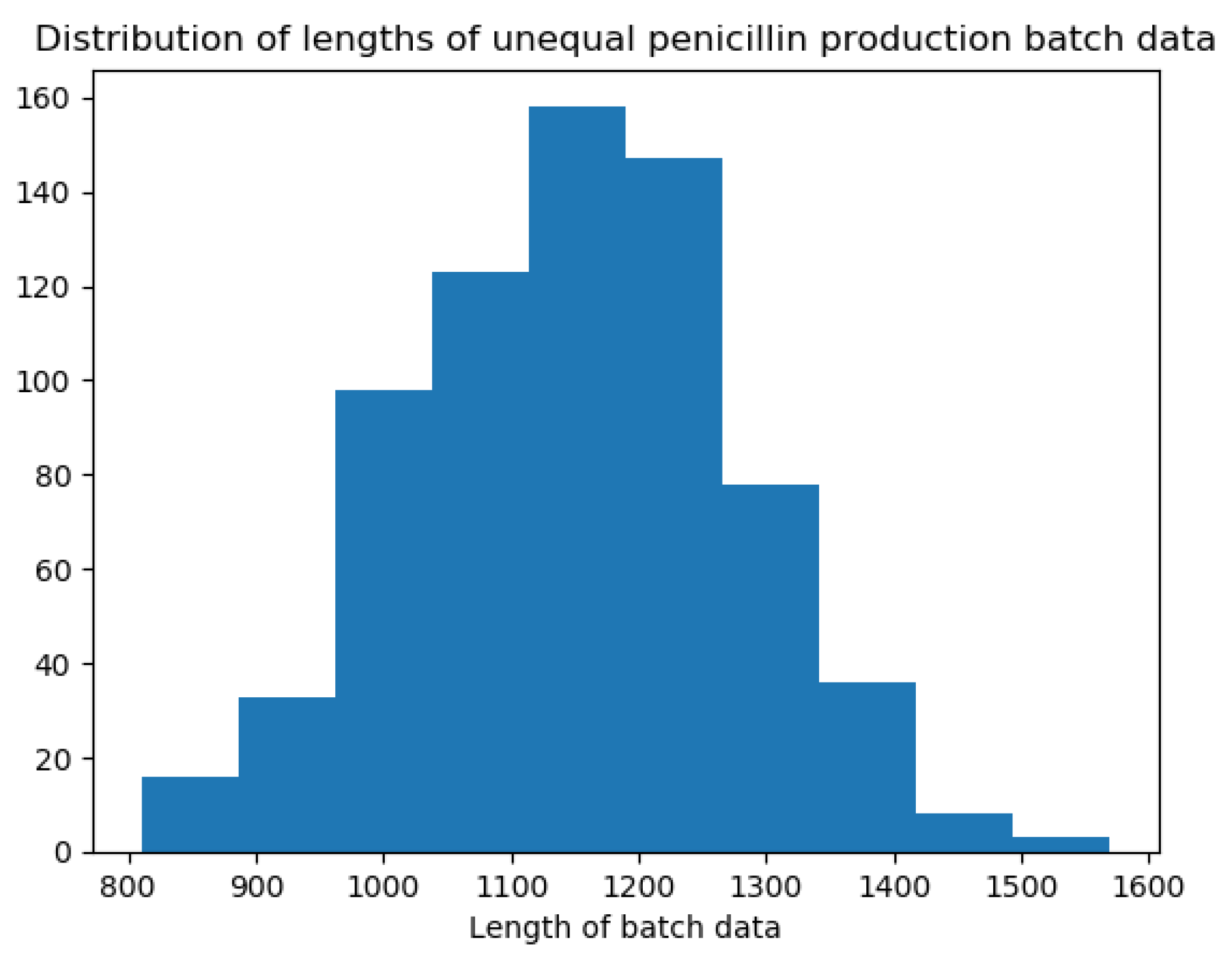
In this study, fifteen process variables impacting penicillin yield are selected for modeling based on the process mechanism [49]. These variables, along with their units, are listed in Table 1. The simulation software generates a dataset comprising seven hundred batches. Out of these, five hundred batches are allocated for the training set, and the remaining two hundred for the testing set. There are wide variations in the batch lengths of the generated dataset, as shown in Figure 5. To address this issue, the data are aligned, and the quality variable is transformed into the process rate, following the methodology introduced in Section 3. This approach allows for calculating penicillin concentration at specific time points by integrating the estimated values over a fixed time window after estimation.

4.3. Sensor Faults

Due to the large number of sensors involved in the process, sensor failure has also become critical in affecting the estimation accuracy of the soft sensor model. Among the variables chosen for modeling, dissolved oxygen concentration is an essential factor affecting fermentation. If the dissolved oxygen concentration is too low, the penicillin production rate decreases dramatically. Conversely, an excessively high concentration of dissolved oxygen weakens the respiratory strength of penicillin, which decreases and adversely affects the production rate. Overall, the sensor failure of dissolved oxygen concentration seriously affects the performance of the soft sensor model for penicillin production. Therefore, the failure of this sensor is selected as a representative case for analysis in this study.
There are various types of sensor failures in industrial processes [50]. In this paper, abrupt offset (caused by impurities) and slow drift of sensors (aging of the optics) have been chosen to focus on. The decision was made for several core reasons. First, these two types of faults are common in many industrial batch processes, and their impacts are progressive, meaning that they can gradually deteriorate product quality and process stability without being recognized and corrected promptly. In addition, drift and offset faults are relatively more complex to detect and diagnose because they are subtle and occur over long periods, which places higher demands on fault detection methods. In contrast, while other types of faults (e.g., erratic, spike, and stuck) are also important, they typically lead to sudden changes that can be more readily identified using current detection techniques. Therefore, this study has chosen to focus our research on drift and offset faults to explore and develop soft sensor algorithms that can tolerate faults in order to improve batch process reliability and product quality.
In order to simulate an abrupt offset, a jump change with a burst with an increase of 10% of the normal fluctuation is added to the dissolved oxygen data in the test set of the simulation data. To simulate the slow drift, concerning the Arrhenius model [51,52], the relationship between measured and actual values is
y ^ = y e ( β t )
where y ^ is the measured value, y is the actual value, t is the duration process time, and the recession factor b e t a is taken as 10 8 .

5. Discussion

5.1. Model Structure and Parameters

The architecture of the proposed model is comprehensively detailed in Section 3. The model’s parameters are optimized using the grid search method, starting with the simplest model configuration and progressively exploring a range of parameters to identify the combination that yields the best results on the test set.
LSTM I consists of two hidden layers, each equipped with 35 neurons. Conversely, LSTM II also consists of two layers, each containing 45 neurons. LSTM I which focuses on process variables is configured with a time step of 5 and an epoch limit of 5000. For LSTM II, the time step is set to 5, while the batch size and maximum epochs are established at 100 and 5000, respectively.
Both LSTM models utilize the mean squared error function as the loss function for optimization and employ the Adam optimizer [53]. The learning rate is set at 0.0002, and an early stopping mechanism is implemented to prevent overfitting.

5.2. Model Comparisons

A LSTM model that incorporates both process variables and historical quality variables fed to the network simultaneously is referred to as concat LSTM. There are 2 hidden layers, each containing 20 neurons. To prevent model overfitting, dropout with a parameter set to 0.3 is applied. The learning rate is 0.0001. The time step of the LSTM is five. Adam optimization is utilized, and the maximum number of epochs is set to 4000.
LSTM-EWMA is a combined method. Exponential weighted moving average (EWMA) is utilized instead of a single-layer LSTM to extract deep information from historical measurement data, and the parameter β is set to 0.8. The use of a single-layer LSTM for extracting process information effectively demonstrates the experiment’s methodology. This approach validates the structural integrity and applicability of the proposed method. The LSTM model consists of two layers, each with 35 neurons. The time step is 3. The learning rate is set to 0.00001, and the maximum number of epochs is 5000. The optimization algorithm chosen is Adam.
To demonstrate the fault tolerance effect of the model, the LSTM model that only uses process variables for modeling, is also used for comparison. The structure and parameter settings of the model are the same as those of the concat LSTM.
Furthermore, to showcase the effectiveness of the proposed method and address the challenge of uneven data, the data are appropriately aligned using padding and resampling methods commonly used in this field. The rest of the modeling method is the same as the proposed method, and comparison experiments are carried out to illustrate its effectiveness.

5.3. Performance Measures

The model’s performance is evaluated by the root mean squared error (RMSE), mean absolute error (MAE) and R-square score ( R 2 ). They are defined as follows:
R M S E = 1 N i = 1 N y ^ i y i 2
M A E = 1 N i = 1 N y ^ i y i 2
R 2 = 1 i = 1 N y ^ i y i 2 i = 1 N y ¯ y i 2
Among them, MAE and RMSE are used to judge the accuracy of the estimation results, and R 2 is used to assess the consistency of the overall trend of the estimation results with the actual values. Compared with MAE, RMSE is related to larger values while ignoring smaller values, so it is more sensitive to outliers.

5.4. Comparison Results on Normal Condition

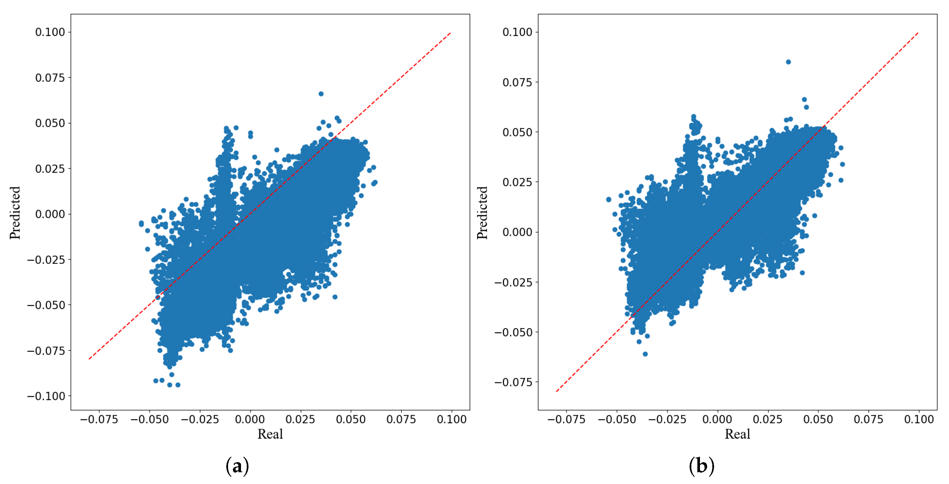
The estimation results of the proposed method for the process rate under the condition of sensor slow drift are shown in Figure 6. Comparing the two subplots, it can be seen that the historical quality variables effectively compensate for the soft sensor estimation results. The results of the proposed method on the training and test sets are shown in Table 2. It can be observed that the algorithm’s results are close on the training set and the test set when there is no sensor failure. However, the algorithm’s performance slightly decreases after a sensor failure occurs.
The comparison of the results within Table 3 shows that the method proposed in this paper is the best performer in terms of RMSE, R-square score, and MAE. LSTM-EWMA method performs suboptimally. The R-square score of the LSTM-EWMA method exceeds 0.85, while the RMSE and MAE are close to those of the proposed method. However, there is some deviation in the estimation of extreme values. The method that relies solely on process data for LSTM modeling is the worst performing, as can be seen in the fact that insufficient information negatively impacts the estimation accuracy of soft sensors. From Table 3, LSTM has nearly double the error compared to the proposed method. Additionally, LSTM is much less effective on the IndPensim dataset, performing slightly worse than concat LSTM. It suggests that the structure of compensation appears to influence estimation accuracy, along with the quality variable information of historical measurements.

5.5. Comparison Results on Fault Condition

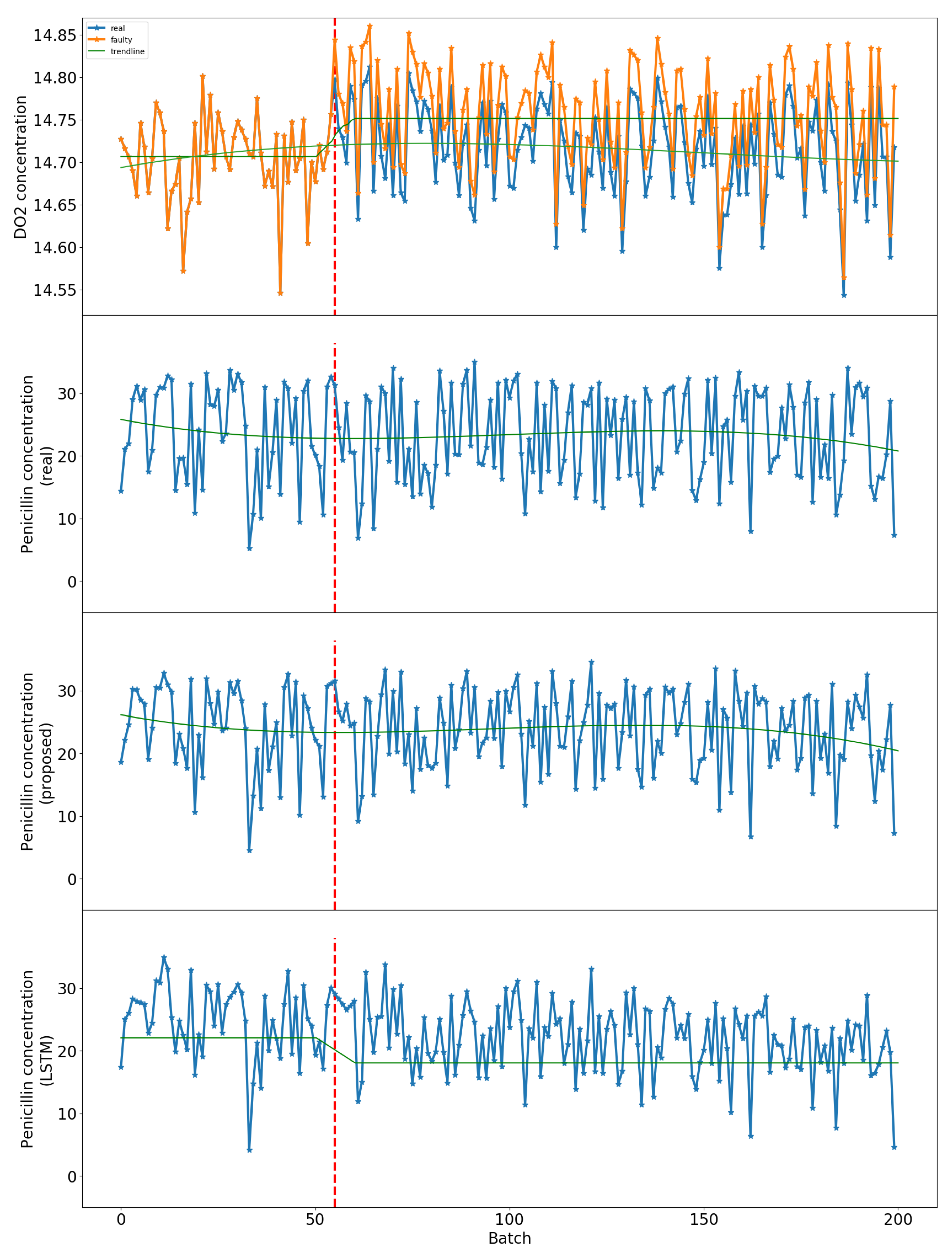
At the abrupt offset of the dissolved oxygen sensor, as indicated in Table 3, a notable decline in the performance of all soft sensors occurs. This illustrates that the abrupt change in dissolved oxygen concentration can affect the final output of penicillin concentration. Taking the R-square score as an example, compared with the normal operation, the accuracy of the proposed method decreases by 1.14%, concat LSTM decreases by 9.27%, and the LSTM method decreases by 10.16%. The result demonstrates that the proposed soft sensor algorithm is fault tolerant. Due to the involvement of EWMA in the compensation, the LSTM-EWMA method still performs second only to the proposed method. In contrast, the LSTM method is significantly affected by sensor failure, with the R-square dropping below 0.8 and the RMSE exceeding 0.01. LSTM is also biased in estimating the trend of the actual values. Comparison of LSTM without compensation illustrates the effect of compensation through Figure 7. It can be seen from batch No. 52 that the dissolved oxygen sensor has failed, resulting in a measured dissolved oxygen content higher than the actual value. The expected values of the quality variables from the soft sensors constructed by LSTM also change abruptly at the corresponding positions, and the estimates are consistently low following the sensor offset. In contrast, the proposed method utilizes faulty sensor data modeling and maintains a smooth trend similar to the actual values. The study demonstrates that the proposed soft sensor algorithm can tolerate failures.
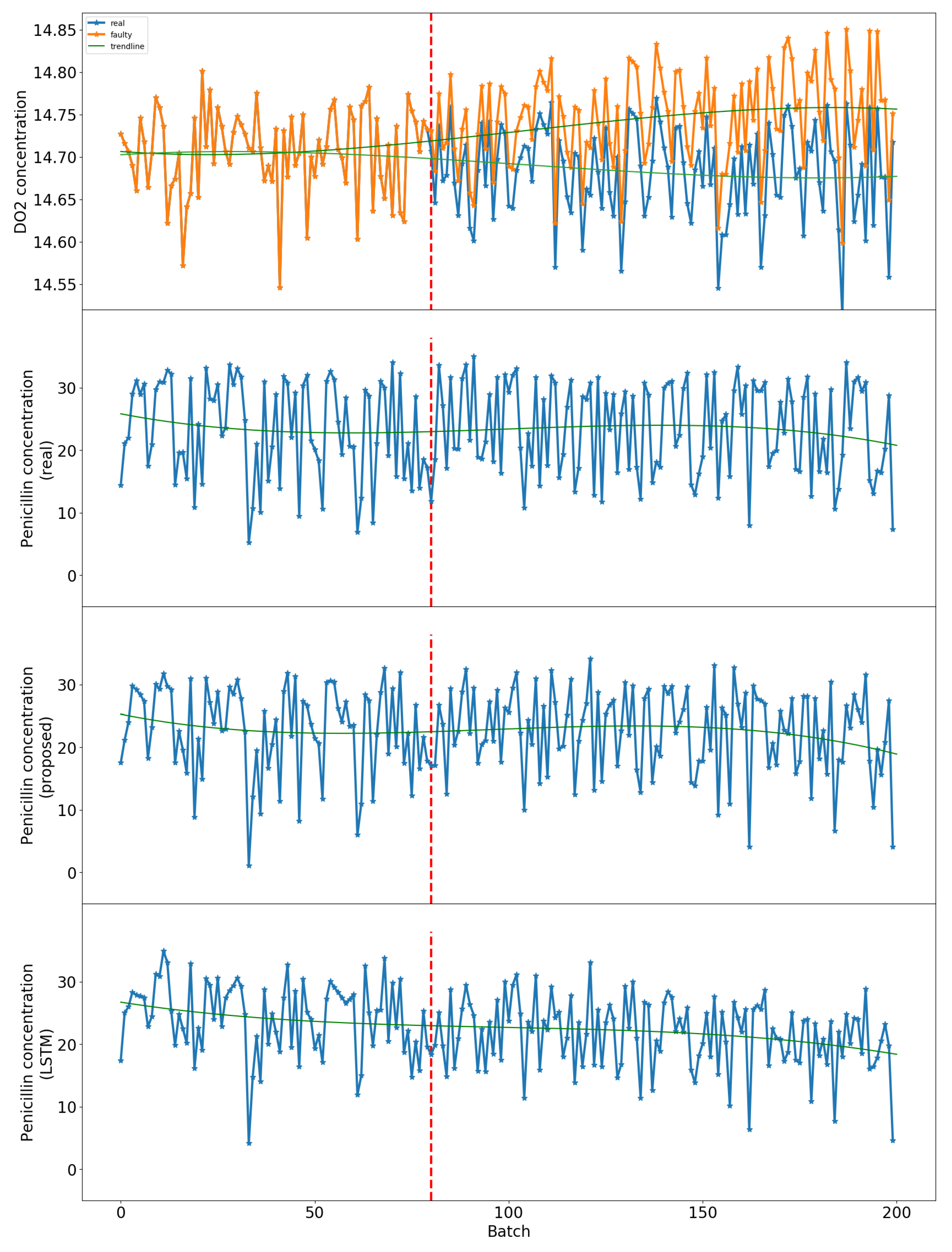
As seen in Table 3, the performance of all methods also decreases with sensor slow drift, illustrating the critical influence of dissolved oxygen concentration on the penicillin concentration produced. Even in the absence of abrupt offset, slow drift introduces a nonlinear bias that can still impact the accuracy of the soft sensor. LSTM continues to perform the worst among the methods, showing the most significant deviation. This indicates the poor robustness of the linear soft sensor in case of sensor failures. From Figure 8, the LSTM estimates show a slowly decreasing drift trend after the failure, reflecting the effect of the sensor failure on the accuracy of the soft sensor estimates. The concat LSTM method also demonstrates a significant decline in effectiveness. The results demonstrate that the LSTM-EWMA method outperforms the LSTM method overall in faulty cases, indicating the effectiveness of fault-tolerant soft sensor compensation using historical measurement data.

5.6. Methods for Aligning Uneven Batches

To illustrate the handling of unequal batches, the most common methods padding and resample are used as comparisons, introduced in Section 2. As can be seen from the Table 4, comparison methods based on the proposed two-layer LSTM soft sensor framework under normal conditions have an R-square score above 0.9. Moreover, the results of the proposed method in this study are again the best among them. The padding method for uneven data is the least effective of the three methods, which shows that the missing information caused by the discarded data affects the estimation accuracy of the soft sensor. Stretching or compressing the data also distorts and destroys the validity of the information. The soft sensors’ estimations decreased when the dissolved oxygen sensor failed. However, the proposed method decreases the least. In fact, it is the most minor degradation among all the methods in fault slow drift fault.

5.7. Endpoint Detection Results

The estimation results of the soft sensor model can be used for endpoint detection of batch production once the quality variable reaches a certain level. In industrial batch processes, reactions have to be terminated timely to prevent waste of resources and decreased production quality due to prolonging the production when the primary reaction has already finished [54]. The specific methods have been described in Section 3. This section only presents the application of the soft sensor model in endpoint detection. The generated penicillin data are still used as a case study. In order to achieve endpoint detection, the actual penicillin yield should be as close as possible to the target value when the soft sensor estimated penicillin yield reaches the target value.
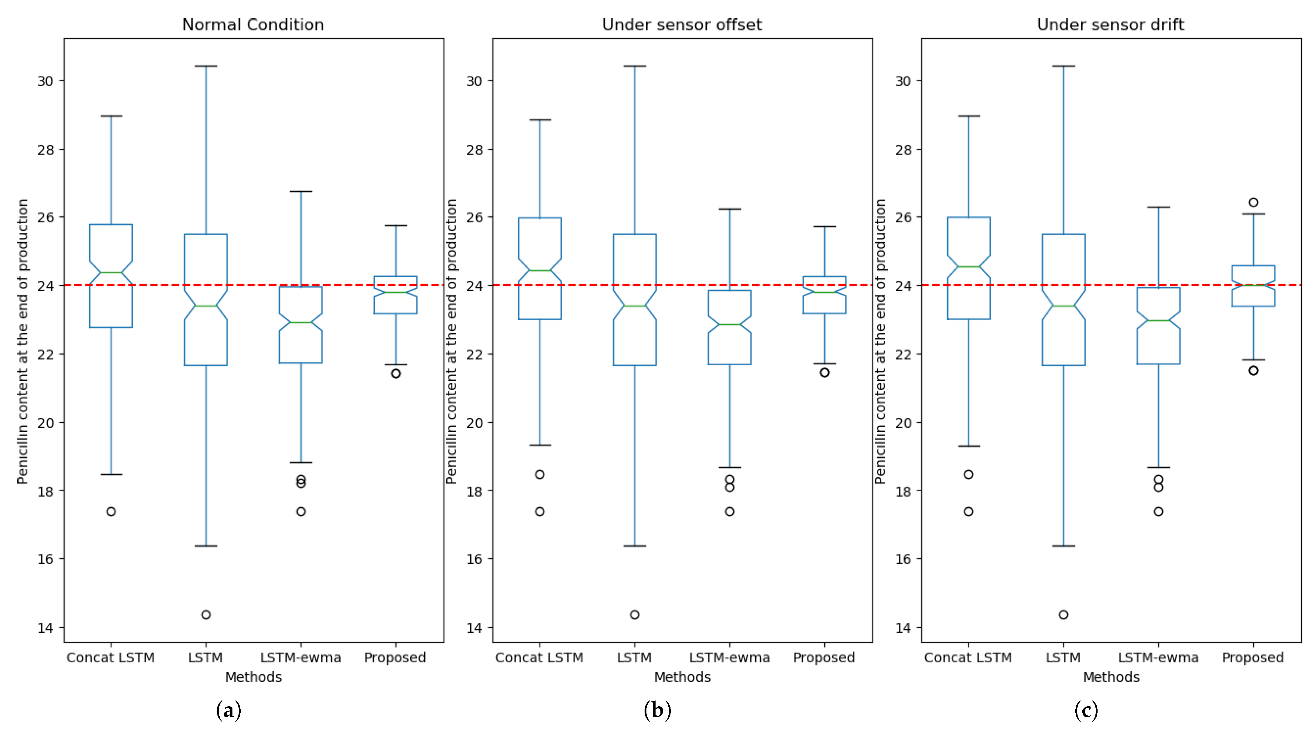
The target yield for the penicillin batch is set at 24 g/L. Production will cease once the penicillin concentration, estimated by the soft sensor model, reaches the target. The actual concentration of penicillin at the moment production stopped for the different models is shown in Figure 9. The MAE of the actual penicillin concentration at the time of production cessation under different conditions regarding the set value is shown in Table 5. It can be seen that the penicillin concentration fluctuates around the target level when various methods are used to stop the process. The discontinuation values of various methods show some deviation. The proposed method shows the least fluctuation near the reference line of 24 g/L. This indicates that the endpoint detection with the proposed method can halt production at the appropriate time to prevent resource wastage. Furthermore, the fluctuation of the LSTM-EWMA method is smaller than that of the concat LSTM. However, the penicillin content at the time when this method stops production almost always did not reach the set value. The penicillin concentration of the LSTM method tends to fall below the intended value and fluctuates with a greater range and error when production is stopped. This indicates that the accuracy is also higher when focusing on control based on a soft sensor model with higher estimation accuracy. It can also be seen from the box plots that the proposed method exhibits the least fluctuation in the termination value, the narrowest box plot, and the median is closest to 24 g/L. Although the box plot corresponding to the final value of the LSTM-EWMA method is also very narrow, the median is noticeably smaller, and there are more outliers. In summary, accurate endpoint detection based on the proposed method can be implemented for the actual penicillin production process.

6. Conclusions

This paper presents a fault-tolerant soft sensor algorithm for uneven batch processes. Uneven batch data, as well as sensor failures—whether abrupt offset or slow drift—affect the accuracy of the soft sensor. The proposed method aligns the uneven batch data by utilizing the differential idea of converting the accumulated quality variable into a process rate. The processed slice data are modeled using the LSTM network. Furthermore, another LSTM network is utilized to model the quality variable of historical batches to compensate for errors caused by sensor failures. The research in this paper focuses on drift and offset faults, which are common in batch processes and significantly impact quality. A case study on IndPensim-generated penicillin production batch process data shows that the proposed algorithm is able to robustly estimate the penicillin concentration when the dissolved oxygen sensor fails. Comparison experiments also demonstrate the effectiveness of the idea presented in this paper for handling uneven batch data compared to other common methods. This paper also employs the soft sensor model for endpoint detection of the penicillin production process, which outperforms other comparative methods. Since the proposed algorithm is data-driven and easy to migrate, it is also applicable to other batch industrial production processes with sensor failures. Future work will consider including more types of sensor faults to further refine and optimize methods for quality soft sensors.

Author Contributions

Conceptualization, Y.L. and D.N.; methodology, Y.L.; data curation, Y.L.; validation, Y.L. and D.N.; investigation, Y.L. and Z.W.; writing—original draft preparation, Y.L.; writing—review and editing, Y.L. and D.N.; visualization, Y.L.; funding acquisition, D.N. All authors have read and agreed to the published version of the manuscript.

Funding

This research was funded by the financial support from the National Natural Science Foundation of China under grant number 62173298.

Data Availability Statement

Data are contained within the article.

Conflicts of Interest

The authors declare no conflicts of interest.

Abbreviations

The following abbreviations are used in this manuscript:
LSTMLong short-term memory
PLSPartial least square
SAEsStacked self-encoders
MLRMultiple linear regression
SVRSupport vector regression
ANNArtificial neural network
RNNRecurrent neural network
DNNDeep neural network
CNNConvolutional neural network
EWMAExponential weighted moving average
RMSERoot mean squared error
MAEMean absolute error
R 2 R-square score

References

  1. Hsiao, Y.D.; Kang, J.L.; Wong, D.S.H. Development of Robust and Physically Interpretable Soft Sensor for Industrial Distillation Column Using Transfer Learning with Small Datasets. Processes 2021, 9, 667. [Google Scholar] [CrossRef]
  2. Souza, F.A.; Araújo, R.; Mendes, J. Review of soft sensor methods for regression applications. Chemom. Intell. Lab. Syst. 2016, 152, 69–79. [Google Scholar] [CrossRef]
  3. Wang, D.; Liu, J.; Srinivasan, R. Data-Driven Soft Sensor Approach for Quality Prediction in a Refining Process. IEEE Trans. Ind. Inform. 2010, 6, 11–17. [Google Scholar] [CrossRef]
  4. Hargrove, M.; Wen, S.; Yim, D.; Ruegger, K.E.; Nanja, P.; Sarkar, S.; Lowe, B.; Vincent, B.; Ervin, J.; Fried, D. Review of virtual wafer process modeling and metrology for advanced technology development. J. Micro/Nanopatterning Mater. Metrol. 2023, 22, 031209. [Google Scholar] [CrossRef]
  5. Kang, P.; Lee, H.j.; Cho, S.; Kim, D.; Park, J.; Park, C.K.; Doh, S. A virtual metrology system for semiconductor manufacturing. Expert Syst. Appl. 2009, 36, 12554–12561. [Google Scholar] [CrossRef]
  6. Jiang, Y.; Yin, S.; Dong, J.; Kaynak, O. A review on soft sensors for monitoring, control, and optimization of industrial processes. IEEE Sens. J. 2020, 21, 12868–12881. [Google Scholar] [CrossRef]
  7. Gonzaga, J.; Meleiro, L.A.C.; Kiang, C.; Maciel Filho, R. ANN-based soft-sensor for real-time process monitoring and control of an industrial polymerization process. Comput. Chem. Eng. 2009, 33, 43–49. [Google Scholar] [CrossRef]
  8. Fortuna, L.; Graziani, S.; Xibilia, M.G. Soft sensors for product quality monitoring in debutanizer distillation columns. Control. Eng. Pract. 2005, 13, 499–508. [Google Scholar] [CrossRef]
  9. Hirai, T.; Kano, M. Adaptive virtual metrology design for semiconductor dry etching process through locally weighted partial least squares. IEEE Trans. Semicond. Manuf. 2015, 28, 137–144. [Google Scholar] [CrossRef]
  10. Kang, S.; Kim, D.; Cho, S. Efficient Feature Selection-Based on Random Forward Search for Virtual Metrology modelling. IEEE Trans. Semicond. Manuf. 2016, 29, 391–398. [Google Scholar] [CrossRef]
  11. Dilmi, S. Calcium Soft Sensor Based on the Combination of Support Vector Regression and 1-D Digital Filter for Water Quality Monitoring. Arab. J. Sci. Eng. 2022, 48, 6111–6136. [Google Scholar] [CrossRef]
  12. Liu, Y.; Yu, X.; Zhao, J.; Pan, C.; Sun, K. Development of a Robust Data-Driven Soft Sensor for Multivariate Industrial Processes with Non-Gaussian Noise and Outliers. Mathematics 2022, 10, 3837. [Google Scholar] [CrossRef]
  13. Zhang, F.; Li, N.; Li, L.; Wang, S.; Du, C. A local semi-supervised ensemble learning strategy for the data-driven soft sensor of the power prediction in wind power generation. Fuel 2022, 333, 126435. [Google Scholar] [CrossRef]
  14. Medl, M.; Rajamanickam, V.; Striedner, G.; Newton, J. Development and Validation of an Artificial Neural-Network-Based Optical Density Soft Sensor for a High-Throughput Fermentation System. Processes 2023, 11, 297. [Google Scholar] [CrossRef]
  15. Zhang, D.; Duan, L.; Xu, Y.; Gao, H.; Liu, N. An ANN-based soft-sensor to estimate the sand content of drilling fluid. In Proceedings of the 2022 IEEE 6th Advanced Information Technology, Electronic and Automation Control Conference (IAEAC), Beijing China, 3–5 October 2022; IEEE: Piscataway, NJ, USA, 2022; pp. 1598–1602. [Google Scholar]
  16. Shen, F.; Zheng, J.; Ye, L.; Ma, X. LSTM Soft Sensor Development of Batch Processes with Multivariate Trajectory Based Ensemble Just-in-time Learning. IEEE Access 2020, 8, 73855–73864. [Google Scholar] [CrossRef]
  17. Ke, W.; Huang, D.; Yang, F.; Jiang, Y. Soft sensor development and applications based on LSTM in deep neural networks. In Proceedings of the 2017 IEEE Symposium Series on Computational Intelligence (SSCI), Honolulu, HI, USA, 27 November–1 December 2017; IEEE: Piscataway, NJ, USA, 2017; pp. 1–6. [Google Scholar]
  18. Yuan, X.; Li, L.; Shardt, Y.; Wang, Y.; Yang, C. Deep learning with spatiotemporal attention-based LSTM for industrial soft sensor model development. IEEE Trans. Ind. Electron. 2020, 68, 4404–4414. [Google Scholar] [CrossRef]
  19. Pisa, I.; Santín, I.; Vicario, J.; Morell, A.; Vilanova, R. ANN-Based Soft Sensor to Predict Effluent Violations in Wastewater Treatment Plants. Sensors 2019, 19, 1280. [Google Scholar] [CrossRef]
  20. Lee, K.B.; Kim, C.O. Recurrent feature-incorporated convolutional neural network for virtual metrology of the chemical mechanical planarization process. J. Intell. Manuf. 2018, 31, 73–86. [Google Scholar] [CrossRef]
  21. Yuan, X.; Huang, B.; Wang, Y.; Yang, C.; Gui, W. Deep learning-based feature representation and its application for soft sensor modeling with variable-wise weighted SAE. IEEE Trans. Ind. Inform. 2018, 14, 3235–3243. [Google Scholar] [CrossRef]
  22. Yuan, X.; Ou, C.; Wang, Y.; Yang, C.; Gui, W. Deep quality-related feature extraction for soft sensing modeling: A deep learning approach with hybrid VW-SAE. Neurocomputing 2020, 396, 375–382. [Google Scholar] [CrossRef]
  23. Ahmad, I.; Ayub, A.; Kano, M.; Cheema, I.I. Gray-box Soft Sensors in Process Industry: Current Practice, and Future Prospects in Era of Big Data. Processes 2020, 8, 243. [Google Scholar] [CrossRef]
  24. Zhang, X.; Song, C.; Zhao, J.; Xu, Z.; Deng, X. Deep subdomain learning adaptation network: A sensor fault-tolerant soft sensor for industrial processes. IEEE Trans. Neural Netw. Learn. Syst. 2022, 1–12. [Google Scholar] [CrossRef] [PubMed]
  25. Liu, Y.J.; Ni, D.; Shao, X.; Gong, D.L.; Li, J.J. A hierarchical model-based method for wafer level virtual metrology under process information deficiency. Qual. Eng. 2023, 1–14. [Google Scholar] [CrossRef]
  26. Du, P.; Zhong, W.; Peng, X.; Li, L.; Li, Z. Data-Driven Fault Compensation Tracking Control for Coupled Wastewater Treatment Process. IEEE/CAA J. Autom. Sin. 2023, 10, 294–297. [Google Scholar] [CrossRef]
  27. Yang, X.B.; Jin, X.Q.; Du, Z.M.; Fan, B.; Zhu, Y.H. Optimum operating performance based online fault-tolerant control strategy for sensor faults in air conditioning systems. Autom. Constr. 2014, 37, 145–154. [Google Scholar] [CrossRef]
  28. Xia, Y.; Xu, Y.; Gou, B. Current sensor fault diagnosis and fault-tolerant control for single-phase PWM rectifier based on a hybrid model-based and data-driven method. IET Power Electron. 2020, 13, 4150–4157. [Google Scholar] [CrossRef]
  29. Belchior, C.A.C.; Araújo, R.A.M.; Souza, F.A.A.; Landeck, J.A.C. Sensor-fault tolerance in a wastewater treatment plant by means of ANFIS-based soft sensor and control reconfiguration. Neural Comput. Appl. 2018, 30, 3265–3276. [Google Scholar] [CrossRef]
  30. Chen, H.; Huang, B. Fault-Tolerant Soft Sensors for Dynamic Systems. IEEE Trans. Control. Syst. Technol. 2023, 31, 2805–2818. [Google Scholar] [CrossRef]
  31. Zhang, S.; Zhao, C. Stationarity test and Bayesian monitoring strategy for fault detection in nonlinear multimode processes. Chemom. Intell. Lab. Syst. 2017, 168, 45–61. [Google Scholar] [CrossRef]
  32. Kourti, T. Multivariate dynamic data modeling for analysis and statistical process control of batch processes, start-ups and grade transitions. J. Chemom. 2003, 17, 93–109. [Google Scholar] [CrossRef]
  33. Liu, J.; Chen, J.; Wang, D. Wavelet functional principal component analysis for batch process monitoring. Chemom. Intell. Lab. Syst. 2020, 196, 103897. [Google Scholar] [CrossRef]
  34. Kassidas, A.; MacGregor, J.F.; Taylor, P.A. Synchronization of batch trajectories using dynamic time warping. AIChE J. 1998, 44, 864–875. [Google Scholar] [CrossRef]
  35. Qiu, K.; Wang, J.; Wang, R.; Guo, Y.; Zhao, L. Soft sensor development based on kernel dynamic time warping and a relevant vector machine for unequal-length batch processes. Expert Syst. Appl. 2021, 182, 115223. [Google Scholar] [CrossRef]
  36. CUI, L.; ZHANG, Q.; SHI, Y.; YANG, L.; WANG, Y.; WANG, J.; BAI, C. A method for satellite time series anomaly detection based on fast-DTW and improved-KNN. Chin. J. Aeronaut. 2023, 36, 149–159. [Google Scholar] [CrossRef]
  37. Zhang, Y.; Zhao, X.; Hui, Y.; Liu, K. Online monitoring and fault diagnosis for uneven length batch process based on multi-way orthogonal enhanced neighborhood preserving embedding. Asia-Pac. J. Chem. Eng. 2022, 17, e2763. [Google Scholar] [CrossRef]
  38. Zhang, Y.; Peng, P.; Liu, C.; Xu, Y.; Zhang, H. A sequential resampling approach for imbalanced batch process fault detection in semiconductor manufacturing. J. Intell. Manuf. 2022, 33, 1057–1072. [Google Scholar] [CrossRef]
  39. Wang, K.; Rippon, L.; Chen, J.; Song, Z.; Gopaluni, R.B. Data-driven dynamic modeling and online monitoring for multiphase and multimode batch processes with uneven batch durations. Ind. Eng. Chem. Res. 2019, 58, 13628–13641. [Google Scholar] [CrossRef]
  40. Yuan, X.; Li, L.; Wang, K.; Wang, Y. Sampling-Interval-Aware LSTM for Industrial Process Soft Sensing of Dynamic Time Sequences With Irregular Sampling Measurements. IEEE Sens. J. 2021, 21, 10787–10795. [Google Scholar] [CrossRef]
  41. Xie, W.; Wang, J.; Xing, C.; Guo, S.; Guo, M.; Zhu, L. Variational autoencoder bidirectional long and short-term memory neural network soft-sensor model based on batch training strategy. IEEE Trans. Ind. Inform. 2020, 17, 5325–5334. [Google Scholar] [CrossRef]
  42. Yuan, X.; Li, L.; Wang, Y. Nonlinear dynamic soft sensor modeling with supervised long short-term memory network. IEEE Trans. Ind. Inform. 2019, 16, 3168–3176. [Google Scholar] [CrossRef]
  43. Ma, L.; Zhao, Y.; Wang, B.; Shen, F. A Multi-Step Sequence-to-Sequence Model with Attention LSTM Neural Networks for Industrial Soft Sensor Application. IEEE Sens. J. 2023, 23, 10801–10813. [Google Scholar] [CrossRef]
  44. Bono, F.; Radicioni, L.; Cinquemani, S. A novel approach for quality control of automated production lines working under highly inconsistent conditions. Eng. Appl. Artif. Intell. 2023, 122, 106149. [Google Scholar] [CrossRef]
  45. Ji, C.; Ma, F.; Wang, J.; Sun, W. Profitability related industrial-scale batch processes monitoring via deep learning based soft sensor development. Comput. Chem. Eng. 2023, 170, 108125. [Google Scholar] [CrossRef]
  46. Bajpai, R.; Reuss, M. A mechanistic model for penicillin production. J. Chem. Technol. Biotechnol. 1980, 30, 332–344. [Google Scholar] [CrossRef]
  47. Birol, G.; Ündey, C.; Cinar, A. A modular simulation package for fed-batch fermentation: Penicillin production. Comput. Chem. Eng. 2002, 26, 1553–1565. [Google Scholar] [CrossRef]
  48. Goldrick, S.; Duran-Villalobos, C.A.; Jankauskas, K.; Lovett, D.; Farid, S.S.; Lennox, B. Modern day monitoring and control challenges outlined on an industrial-scale benchmark fermentation process. Comput. Chem. Eng. 2019, 130, 106471. [Google Scholar] [CrossRef]
  49. Gins, G.; Van Impe, J.F.; Reis, M.S. Finding the optimal time resolution for batch-end quality prediction: MRQP—A framework for multi-resolution quality prediction. Chemom. Intell. Lab. Syst. 2018, 172, 150–158. [Google Scholar] [CrossRef]
  50. Jan, S.U.; Lee, Y.D.; Shin, J.; Koo, I. Sensor fault classification based on support vector machine and statistical time-domain features. IEEE Access 2017, 5, 8682–8690. [Google Scholar] [CrossRef]
  51. Tobias, P.A.; Trindade, D. Applied Reliability; CRC Press: Boca Raton, FL, USA, 2011. [Google Scholar]
  52. Suhir, E. Static fatigue lifetime of optical fibers assessed using Boltzmann–Arrhenius–Zhurkov (BAZ) model. J. Mater. Sci. Mater. Electron. 2017, 28, 11689–11694. [Google Scholar] [CrossRef]
  53. Kingma, D.P.; Ba, J. Adam: A Method for Stochastic Optimization. arXiv 2014, arXiv:1412.6980. [Google Scholar]
  54. Offermans, T.; Wijker, T.H.; Folcarelli, R.; Heemskerk, R.; Lamers, P.P.; Proenca, M.; Tran, T.N.; Buydens, L.M.C.; Jansen, J.J. ENDBOSS: Industrial endpoint detection using batch-specific control spaces of spectroscopic data. Chemom. Intell. Lab. Syst. 2021, 209, 209. [Google Scholar] [CrossRef]
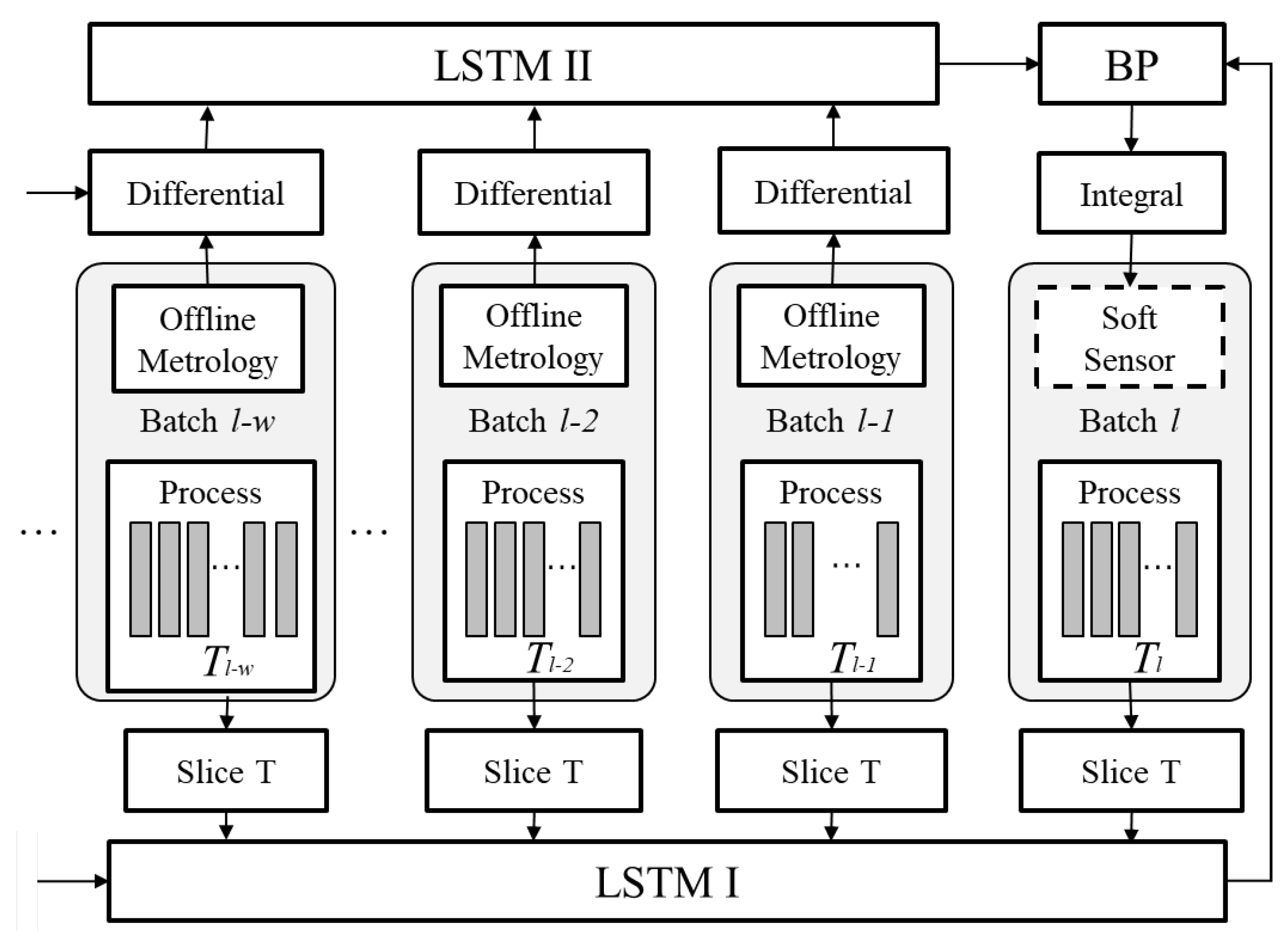
Figure 1. Model structure of the LSTM-based soft sensor algorithm.
Processes 12 00495 g001
Figure 2. Structure of LSTM I in the proposed soft sensor algorithm.
Processes 12 00495 g002
Figure 3. Structure of LSTM II in the proposed soft sensor algorithm.
Processes 12 00495 g003
Figure 4. The main inputs and outputs from the simulation IndPensim [48].
Processes 12 00495 g004
Figure 5. Length distribution of generated uneven batch data.
Processes 12 00495 g005
Figure 6. Comparison of estimation and actual values of rates before and after compensation. (a) Before compensation. (b) After compensation.
Processes 12 00495 g006
Figure 7. Comparison of estimation results for soft sensors under sensor offset.
Processes 12 00495 g007
Figure 8. Comparison of estimation results for soft sensors under sensor drift.
Processes 12 00495 g008
Figure 9. Comparison of endpoint detection results by different methods. (a) Normal condition. (b) Abrupt offset. (c) Slow drift fault.
Processes 12 00495 g009
Table 1. List of process variables for soft sensor modeling in the case study.
Variable
Time (h)Base flow rate (L/h)Vessel weight (Kg)
Aeration rate (L/h)Cooling water flow rate (L/h)PH
Agitator RPM (RPM)Heating water flow rate (L/h)Temperature (K)
Sugar feed rate (L/h)Dissolved oxygen concentration (mg/L)Vessel Volume (L)
Acid flow rate (L/h)Carbon dioxide in off-gas (%)Oxygen in off-gas (%)
Table 2. The results of the proposed method on the train and test set.
TrainTest
NormalNormalOffsetDrift
RMSE0.005800.005790.006230.00602
R 2 0.933670.933550.922920.92813
MAE0.003780.003790.004910.00397
Table 3. Comparison of estimation results for soft sensors under different conditions.
MethodsRMSE R 2 MAE
NormalOffsetDriftNormalOffsetDriftNormalOffsetDrift
Proposed0.005790.006230.006020.933550.922920.928130.003790.004910.00397
LSTM-ewma0.007210.007470.007800.896800.889270.879430.005180.005320.00563
Concat LSTM0.008090.010300.009770.870200.789520.810660.005410.007250.00684
LSTM0.010330.011380.012140.763720.707670.683920.008920.010240.01114
Table 4. Comparison of estimation results from methods for aligning uneven batches.
MethodsRMSE R 2 MAE
NormalOffsetDriftNormalOffsetDriftNormalOffsetDrift
Proposed0.005790.006230.006020.933550.922920.928130.003790.004910.00397
Padding0.007000.008390.006830.904270.862370.887500.005420.005910.00562
Resample0.006790.007930.007360.910060.877060.894250.005210.005920.00502
Table 5. Mean absolute error in different methods of soft sensors for endpoint detection of stopped production.
NormalOffsetDrift
Proposed0.641230.655970.70415
LSTM-EWMA1.666021.689731.68063
Concat LSTM1.792871.808911.83912
LSTM2.030242.143832.16533
Disclaimer/Publisher’s Note: The statements, opinions and data contained in all publications are solely those of the individual author(s) and contributor(s) and not of MDPI and/or the editor(s). MDPI and/or the editor(s) disclaim responsibility for any injury to people or property resulting from any ideas, methods, instructions or products referred to in the content.